https://doi.org/10.5194/tc-12-1307-2018
© Author(s) 2018. This work is distributed under the Creative Commons Attribution 4.0 License.
Open-source algorithm for detecting sea ice surface features
in high-resolution optical imagery
Nicholas C. Wright1and Chris M. Polashenski1,2
1Thayer School of Engineering, Dartmouth College, Hanover, NH, USA
2U.S. Army Cold Regions Research and Engineering Laboratories, Hanover, NH, USA
Correspondence:Nicholas C. Wright ([email protected]) Received: 31 July 2017 – Discussion started: 18 September 2017
Revised: 22 February 2018 – Accepted: 11 March 2018 – Published: 12 April 2018
Abstract.Snow, ice, and melt ponds cover the surface of the Arctic Ocean in fractions that change throughout the sea-sons. These surfaces control albedo and exert tremendous influence over the energy balance in the Arctic. Increas-ingly available meter- to decimeter-scale resolution optical imagery captures the evolution of the ice and ocean surface state visually, but methods for quantifying coverage of key surface types from raw imagery are not yet well established. Here we present an open-source system designed to provide a standardized, automated, and reproducible technique for pro-cessing optical imagery of sea ice. The method classifies sur-face coverage into three main categories: snow and bare ice, melt ponds and submerged ice, and open water. The method is demonstrated on imagery from four sensor platforms and on imagery spanning from spring thaw to fall freeze-up. Tests show the classification accuracy of this method typically ex-ceeds 96 %. To facilitate scientific use, we evaluate the mini-mum observation area required for reporting a representative sample of surface coverage. We provide an open-source dis-tribution of this algorithm and associated training datasets and suggest the community consider this a step towards stan-dardizing optical sea ice imagery processing. We hope to en-courage future collaborative efforts to improve the code base and to analyze large datasets of optical sea ice imagery.
1 Introduction
The surface of the sea ice–ocean system exhibits many dif-ferent forms. Snow, ice, ocean, and melt ponds cover the sur-face in fractions that change throughout the seasons. The rel-ative fractions of these surfaces covering the Arctic ocean
are undergoing substantial change due to rapid loss of sea ice (Stroeve et al., 2012), increase in the duration of melt (Markus et al., 2009; Stroeve et al., 2014), decrease in sea ice age (Maslanik et al., 2011), and decrease in sea ice thick-ness (Kwok and Rothrock, 2009; Laxon et al., 2013) over recent decades. As a whole, the changes are reducing albedo and enhancing the absorption of solar radiation, triggering an ice albedo feedback (Curry et al., 1995; Perovich et al., 2008; Pistone et al., 2014). Large-scale remote sensing has been instrumental in documenting the ongoing change in ice extent (Parkinson and Comiso, 2013), thickness (Kurtz et al., 2013; Kwok and Rothrock, 2009; Laxon et al., 2013), and surface melt state (Markus et al., 2009). An increasing fo-cus on improving prediction of future sea ice and climate states, however, has also created substantial interest in better observing, characterizing, and modeling the processes that drive changes in albedo-relevant sea ice surface conditions such as melt pond formation, which occur at smaller length scales. For these, observations that resolve surface conditions explicitly are needed to understand the underlying causes of the seasonal and spatial evolution of albedo in a more sophis-ticated way.
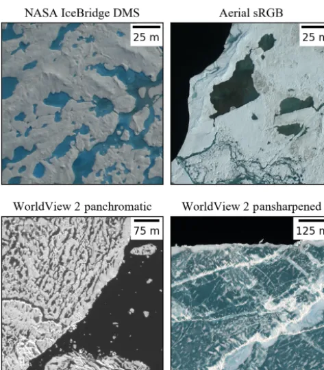
Figure 1.Examples of imagery from each of the four imaging plat-forms that we seek to classify in this study. Each type of imagery has either a different spatial resolution or different levels spectral information available.
scale from manned ground campaigns is both time consum-ing and impractical. Remote sensconsum-ing provides a more viable approach for studying these multi-kilometer areas. High-resolution optical imagery (e.g., Fig. 1) visually captures the surface features of interest, but the methods for analyzing this imagery remain under-developed.
The need for remote sensing methods enabling quantifi-cation of meter-scale sea ice surface characteristics has been well recognized, and efforts have been made to address it. Recent developments in remote sensing of sea ice surface conditions fall into two categories: (1) methods using low– medium resolution satellite imagery (i.e., having pixel sizes larger than the typical ice surface feature size) with spec-tral un-mixing type algorithms to derive aggregate measures of sub-pixel phenomena (e.g., for melt ponds Markus et al., 2003; Rösel et al., 2012; Rösel and Kaleschke, 2011; Tschudi et al., 2008) and (2) methods using higher-resolution satel-lite or airborne imagery (i.e., having pixel size smaller than the typical scale of ice surface features) that is capable of explicitly resolving features (e.g., Arntsen et al., 2015; Fet-terer and Untersteiner, 1998; Inoue et al., 2008; Kwok, 2014; Lu et al., 2010; Miao et al., 2015; Perovich et al., 2002b; Renner et al., 2014; Webster et al., 2015). The first category, those derived from low–medium resolution imagery, have notable strengths in their frequent sampling and basin-wide coverage. They cannot, however, provide detailed statistics
on the morphology of surface features necessary for assess-ing our process-based understandassess-ing and have substantial un-certainty due to ambiguity in spectral signal un-mixing. The second category – observations at high resolutions which ex-plicitly resolve surface properties – can provide these de-tailed statistics but were historically limited by a dearth of data acquisitions. Recent increases in imagery availability from formerly classified defense (Kwok, 2014) or commer-cial satellites (e.g., DigitalGlobe), and increases in manned flights over the Arctic (e.g., IceBridge, SIZRS) have substan-tially reduced this constraint for optical imagery. While high-resolution imagery still does not provide basin-wide cover-age, likely increases in collection of imagery from UAVs (DeMott and Hill, 2016) and increases in satellite imag-ing bandwidth (e.g., DigitalGlobe WorldView 4 launched in 2016) suggest that availability of high-resolution imagery will continue to increase.
Processing high-resolution sea ice imagery to derive use-ful metrics quantifying surface state, however, remains a ma-jor hurdle. Recent years have seen numerous publications demonstrating the success of various processing techniques for optical imagery of sea ice on limited test cases (e.g., In-oue et al., 2008; Kwok, 2014; Lu et al., 2010; Miao et al., 2015; Perovich et al., 2002b; Renner et al., 2014; Webster et al., 2015). None of these techniques, however, have been adopted as a standard or been used to produce large-scale datasets, and validation has been limited. Furthermore, no single method has been used to process data from multi-ple sensor platforms or documented and released for wide-spread community use. These issues must be addressed to enable in large-scale production-type image processing and use of high-resolution imagery as a sea ice monitoring tool.
A unique aspect of high-resolution sea ice imagery datasets, which differs from most satellite remote sensing, is the quantity of image sources and data owners. Distributed collection and data ownership means centralized processing of imagery to produce a single product is unlikely. Instead, we believe that distributed processing by dataset owners is more likely and the community therefore has a substantial need for a shared, standard processing protocol. Successful creation of such a processing protocol would increase im-agery analysis and result in the production of datasets suit-able for ingestion by models to validate surface process pa-rameterizations. In this paper, we assess previous publica-tions detailing image processing methods for remote sensing and present a novel scheme that builds from the strengths and lessons of prior efforts. Our resulting algorithm, the Open Source Sea-ice Processing (OSSP) algorithm, is presented as a step toward addressing the community need for a standard-ized methodology and released in an open-source implemen-tation for use and improvement by the community.
con-sistent results in a standardized output format, and (3) be able to produce equivalent geophysical parameters from a range of disparate image acquisition methods. To meet these goals, we have packaged OSSP in a user-friendly format, with clear documentation for start-up. We include a set of default parameters that should meet most user needs, per-mitting processing of pre-defined image types with minimal setup. The algorithm parameters are tunable to allow more advanced users to tailor the method to their specific imagery input. We chose an open-source format to enhance the abil-ity for the communabil-ity to explore and improve the code rela-tive to commercial software. Herein, we discuss how we ar-rived at the particular technique we use, and why it is su-perior to some other possible mechanisms. We then demon-strate the ability of this algorithm to analyze imagery of dis-parate sources by showing results from high-resolution Dig-italGlobe WorldView satellite imagery in both panchromatic and pansharpened formats, aerial sRGB (standard red, green, blue) imagery, and NASA Operation IceBridge DMS (Digi-tal Mapping System) optical imagery. In this paper, we clas-sify imaged areas into three surface types: snow and ice, melt ponds and submerged ice, and open water. The algorithm is, however, suitable for classifying any number of categories, should a user be interested in different surface types, and might be adapted for use on imagery of other surface types.
2 Algorithm design
Two core decisions were faced in the design of this image classification scheme: (1) whether to analyze the image by individual pixels or to analyze objects constructed of similar, neighboring pixels, and (2) which algorithm to use for the classification of these image units.
Prior work in terrestrial remote sensing applications has shown that object-based classifications are more accu-rate than single pixel classifications when analyzing high-resolution imagery (Blaschke, 2010; Blaschke et al., 2014; Duro et al., 2012; Yan et al., 2006). In this case, “high res-olution” has a specific definition dependent on the relation-ship between the size of pixels and objects of interest. An image is high resolution when surface features of interest are substantially larger than pixel resolution and therefore are composed of many pixels. In such imagery, objects, or groups of pixels constructed to contain only similar pixels (i.e., a single surface type), can be analyzed as a set. The meter–decimeter-resolution imagery meets this definition for features like melt ponds and ice floes. Object-based classi-fication enables an algorithm to extract information about image texture and spatial correlation within the pixel group, information that is not available in single pixel-based classi-fications and can enhance accuracy of surface type discrim-ination. Furthermore, object-based classifications are much better at preserving the size and shape of surface cover re-gions. Classification errors of individual pixel schemes tend
to produce a “speckled” appearance in the image classifica-tion with incorrect pixels scattered across the image. Errors in object-based classifications, meanwhile, appear as entire objects that are mislabeled (Duro et al., 2012). Since our in-tent is not only to process high-resolution imagery and pro-duce measurements of the areal fractions of surface type re-gions but also to enable analysis of the size and shape of ice surface type regions (e.g., for floe size or melt pond size de-termination), the choice of object-based classification over pixel-based was clear.
A wide range of algorithms were considered for classi-fying image objects. We first considered the use of super-vised versus an unsupersuper-vised classification schemes. Unsu-pervised schemes were rejected as they produce inconsistent, non-intercomparable results. These schemes, such as cluster-ing algorithms, group observations into a predefined number of categories – even if not all feature types of interest are present in an image. For example, an image containing only snow-covered ice will still be categorized into the same num-ber of classes as an image with snow, melt ponds, and open water together – resulting in multiple classes of snow. Since the boundary between classes also changes in each image, standardizing results across imagery with different sources and of scenes with different feature content would be chal-lenging at best.
Supervised classification schemes instead utilize a set of known examples (called training data) to assign a classifica-tion to unknown objects based on similarity to user-identified objects. Supervised classification schemes have several ad-vantages. They can produce fixed surface type definitions, allow for more control and fine tuning of the algorithm, im-prove in skill as more points are added to the training data, and allow users to choose what surface characteristics they wish to classify. While many machine learning techniques have shown high accuracy in remote sensing applications (Duro et al., 2012), we selected a random forest machine learning classifier over other supervised learning algorithms for its ability to handle nonlinear and categorical training in-puts (Breiman, 2001; DeFries, 2000; Pal, 2005), resistance to outliers in the training dataset (Breiman, 1996), and relative ease of implementation.
standardized method. Our hope is to continue development of the algorithm with contributions and suggestions from the sea ice community.
3 Methods
3.1 Image collection and preprocessing
The imagery used to test the algorithm was selected from four distinct sources in order to assess the algorithm’s abil-ity to deliver consistent and intercomparable measures of geophysical parameters. We chose high-resolution satellite imagery from DigitalGlobe’s WorldView constellation in panchromatic and eight-band multispectral formats, NASA Operation IceBridge Digital Mapping System optical im-agery, and aerial sRGB imagery collected using an aircraft-mounted standard DLSR camera as part of the SIZONet project. We first demonstrate the technique’s ability to han-dle imagery representing all stages of the seasonal evolution of sea ice conditions on a series of 22 panchromatic satellite images collected between March and August 2014 at a single site in the Beaufort Sea: 72.0◦N, 128.0◦W. We then process four multispectral WorldView 2 images of the same site, each collected coincident with a panchromatic image and compare results to assess the benefit of spectral information. Finally, we process a set of 20 sRGB images and 20 IceBridge DMS images containing a variety of sea ice surface types to illus-trate the accuracy of the method on aerial image sources. The imagery sources chosen for this analysis were selected to be representative of the variation that exists in optical imagery of sea ice, but there is an abundance of image data that can be processed with this technique.
The satellite images were collected by tasking WorldView 1 and WorldView 2 Digital Globe satellites over fixed lo-cations in the Arctic. Tasking requests were submitted to DigitalGlobe with the support and collaboration of the Po-lar Geospatial Center. The panchromatic bands of World-View 1 and 2 both have a spatial resolution of 0.46 m at nadir. The WorldView 1 satellite panchromatic band sam-ples the visible spectrum between 400 and 900 nm, while the WorldView 2 satellite panchromatic band samples between 450 and 850 nm. In addition, WorldView 2 has eight mul-tispectral bands at 1.84 m nadir resolution, capturing bands within the range of 400 to 1040 nm. Each WorldView im-age captures an area of ∼700–1300 km2. Of the 22 use-able panchromatic collections at the site, 15 were completely cloud-free, while 7 of the images were partially cloudy. Im-ages with partial cloud cover were manually masked and cloud-covered areas were excluded from analysis. The aerial sRGB imagery was captured along a 100 km long transect to the north of Utqia˙gvik, Alaska, with a Nikon D70 DSLR mounted at nadir to a light airplane during June 2009. The IceBridge imagery was collected in July 2016 near 73◦N, 171◦W with a Canon EOS 5D Mark II digital camera. We
utilize the L0 (raw) DMS IceBridge imagery, which has a 10 cm spatial resolution when taken from 1500 ft (457.2 m) altitude (Dominguez, 2010, updated 2017).
Each satellite image was orthorectified to mean sea level before further processing. Orthorectification corrects for im-age distortions caused by off-nadir acquisition angles and produces a planimetrically correct image that can be ac-curately measured for distance and area. Due to the rela-tively low surface roughness of both multiyear and first year sea ice (Petty et al., 2016), errors induced by ignoring the real topography during orthorectification are small. Multi-spectral imagery was pansharpened to the resolution of the panchromatic imagery. Pansharpening is a method that cre-ates a high-resolution multispectral image by combining in-tensity values from a higher-resolution panchromatic image with color information from a lower-resolution multispec-tral image. The pansharpened imagery used here was cre-ated using a “weighted” Brovey algorithm. This algorithm resamples the multispectral image to the resolution of the panchromatic image, then each pixel’s value is multiplied by the ratio of the corresponding panchromatic pixel value to the sum of all multispectral pixel values. The orthorectifica-tion and pansharpening scripts were developed by the Polar Geospatial Center at the University of Minnesota and utilize the GDAL (Geospatial Data Abstraction Library) image pro-cessing tools (GDAL, 2016). All imagery used was rescaled to the full 8 bit color space for improved contrast and view-ing. No other preprocessing was done to the aerial sRGB im-agery or IceBridge DMS imim-agery.
3.2 Image segmentation
Preprocessed image
Sobel filter
Gradient image
Watershed transformation
Segmented image
Random forest classification
Classified image
Local minima
Training set creation Region seeds
Amplify and threshold
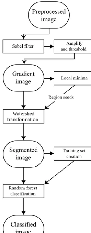
Figure 2.Flow diagram depicting the steps taken to classify an im-age in the OSSP algorithm.
filter, and eliminates weaker edges. The amplification factor and gradient threshold percentage are both tuning parame-ters, which can be adjusted to properly segment images based on the input image and the strength of edges sought.
The strongest edges in optical imagery of sea ice are typ-ically the ocean–ice interface, followed by melt pond–ice boundaries, then ice ridges and uneven ice surfaces. In gen-eral, the more edges detected, the more segmented the image will become, and the more computational resources required to later classify the increased number of image objects. On the other hand, an under-segmented image may miss the nat-ural boundaries between surfaces. Under-segmentation intro-duces classification error because an object containing two surface types cannot be correctly classified. An optimally segmented image is one which captures all the natural surface boundaries with minimal over-segmentation (i.e., boundaries placed in the middle of features). The appropriate
parame-ters for our imagery were tuned by visual inspection of the segmentation results. In such inspection, desired segmen-tation lines are manually drawn, and algorithm-determined segmentation lines are overlain and evaluated for complete-ness.
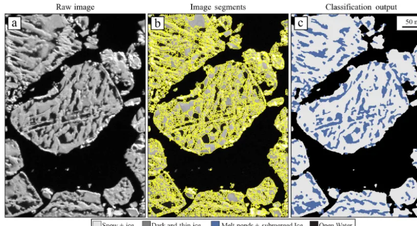
The result of the edge detection is a gradient map that marks the strength of edges in the image. We use a water-shed segmentation technique to build complete objects based on edge locations and intensity (van der Walt et al., 2014). We first calculate all local minimum values in the gradient image, where a marker is then placed to indicate the origin of watershed regions. Each region then begins iteratively ex-panding in all directions of increasing image gradient until encountering a local maximum in the gradient image or en-countering a separately growing region. This continues until every pixel in the image belongs to a unique set. With the proper parameter selection, each object will represent a sin-gle surface type. It is often the case that some areas will be over-segmented (i.e., a single surface feature represented by multiple objects). Over-segmentation can either be ignored or objects can be recombined if they meet similarity criteria in an effort to save computational resources. Here we chose to classify objects without recombination. Figure 3b shows the detected edges overlain on top of the input image.
The watershed segmentation algorithm benefits from the ability to create objects of variable size. Large objects are built in areas of low surface variability, while many small objects are created in areas of high variability. This variable object sizing is well suited to sea ice surface classification because the variability of each surface type occurs at differ-ent scales. Areas of open water and snow-covered first-year ice, for example, can often be found in large expanses, while areas that contain melt ponds, ice ridges, or rubble fields fre-quently cover small areas and are tightly intermingled with other surface types. Variable object sizes give the fine detail needed to capture surfaces of high heterogeneity in their full detail, while limiting over segmentation of uniform areas. 3.3 Segment classification
3.3.1 Overview
Figure 3.Visual representation of important steps in the image processing workflow. Panel(a)shows preprocessed panchromatic WorldView 2 satellite imagery, taken on 1 July 2014. In panel(b), outlines of the image objects created by our edge detection and watershed transfor-mation are shown overlain on top of the image in panel(a). Panel(c)shows the result of replacing each object with a value corresponding to the prediction of the random forest classifier.
one of many available machine learning approaches and oth-ers may also be suitable.
3.3.2 Surface type definitions
Another key challenge to quantitatively monitoring sea ice surface characteristics from high-resolution imagery is a lack of standardized surface type definitions. We noted above that high-resolution sea ice imagery comes from many sources, each with different characteristics. As we will see below, each image source will need to have its own training set created by expert human classifiers. The human classifier must train the algorithm according to definitions of each sur-face type that are broadly agreed upon in the community for the algorithm to be successful in producing intercom-parable datasets. While at first the definitions of open wa-ter, ice, and melt ponds might seem intuitive, many experts in the cryosphere community have differing opinions, espe-cially on transitional states. Deciding where to delineate tran-sitional states is important to standardization. We have estab-lished the following definitions for the three surface types we sought to separate, binning transitional states in a manner most consistent with their impact on albedo. Our surface type definitions focus on the behavior of a surface in absorption of shortwave radiation and radiative energy transfer.
– (1) Open Water (OW): applied to surface areas that had zero ice cover as well as those covered by an unconsol-idated frazil or grease ice.
– (2) Melt Ponds and Submerged Ice (MPS): applied to surfaces where a liquid water layer completely sub-merges the ice.
– (3) Ice and Snow (I+S): applied to all surfaces covered by snow or bare ice, as well as decaying ice and snow that is saturated but not submerged.
The definition of melt ponds includes the classical defini-tion of melt ponds where meltwater is trapped in isolated patches atop ice, as well as optically similar ice submerged near the edge of a floe. While previous work separates these categories (e.g., Miao et al., 2015) we did not attempt to break these “pond” types because the distinction is unimpor-tant from a shortwave energy balance (albedo) perspective. We further refined the Ice and Snow category into two sub-categories:
– (3a) Thick Ice and Snow: applied during the freezing season to ice appearing to the expert classifier to be thicker than 50 cm or having an optically thick snow cover and to ice during the melt season covered by a drained surface scattering layer (Perovich, 2005) of de-caying ice crystals.
In some prior publications (e.g., Polashenski et al., 2012) la-bel 3b was described as “slushy bare ice”. We acknowledge that the boundary between the ice and snow sub-categories is often more a continuum than a defined border but note that distinguishing the two types is useful for algorithm ac-curacy. Dividing the ice/snow type creates two relatively ho-mogeneous categories rather than a single larger category with large internal differences. A user only interested in the categories of ice, ponds, and open water could simply re-combine them, as we have done for analysis. A temporary fourth category was created to classify shadows over snow or ice. This category is used exclusively as an intermediate step in processing that allows us to bypass masking shadow regions (e.g., Webster et al., 2015). As this was not designed to be a stand-alone classification category (as opposed to Miao et al., 2015, 2016), objects classified as a shadow were merged into the ice/snow category (as is done in Webster et al., 2015). Any misclassifications due to shadow cover are accounted for in measurements of overall classification ac-curacy (Sect. 5.1).
3.3.3 Attribute selection
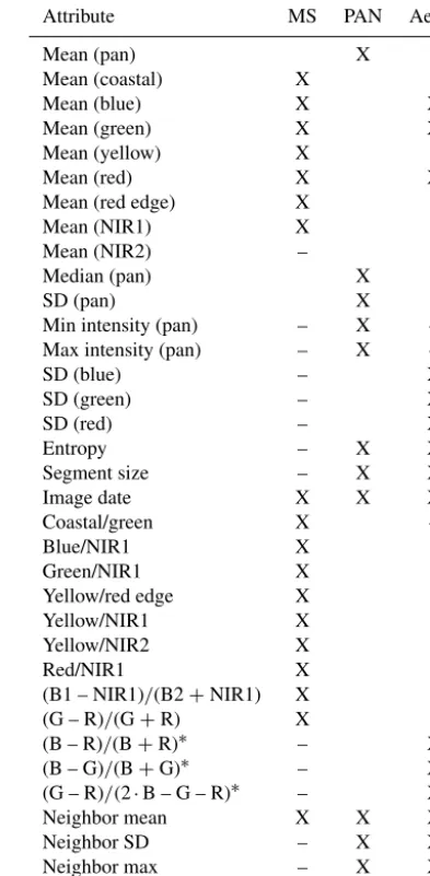
Attributes are quantifiable measures of image object prop-erties used by the classifier in discriminating surface types. An enormous array of possible attributes could be calculated for each image object and could be calculated in many ways. Examples of properties that could be quantified as attributes include values of the enclosed pixels, the size and shape of the object, and values of adjacent pixels. The calculation of pixel values aggregated by image objects takes advantage of the additional information held in the pixel group (as com-pared to individual pixels). We have compiled a list repre-senting a relevant subset of such attributes that can be used to distinguish different surface types in Table 1. We included a selection of attributes similar to those used in previous publi-cations (e.g., Miao et al., 2015), as well as attributes we have developed specifically for our algorithm.
Each image source provides unique information about the surface and it can be expected that a different list of attributes will be optimal for classification of each image type – even though we seek the same geophysical parameters. As high-resolution satellite images can have millions of image ob-jects, calculating the attributes of each object quickly be-comes computationally expensive. We have, therefore, deter-mined those that are most valuable for classifying each image type to use in our classification. For example, pansharpened WorldView 2 imagery has eight spectral bands which can in-form the classification, while panchromatic versions of the same image have only a single band. Our goal was to select a combination of attributes that describe the intensity and tex-tural characteristics of the object itself, and of the area sur-rounding the object. Table 1 indicates which attributes were selected for use in classifying each image type.
Table 1. Attributes used for classifying each of the three image types. X marks indicate attributes that were used for that image type. Dash marks indicate attributes that are available but were not found to be sufficiently beneficial in the classification to merit inclusion under our criteria. Empty areas indicate attributes that are not avail-able on that image type (e.g., band ratios on a panchromatic image). NIR is the near-infrared wavelength. B1 is the costal WorldView band, and B2 is the blue band. R, G, and B, stand for red, green, and blue, respectively.
Attribute MS PAN Aerial
Mean (pan) X
Mean (coastal) X
Mean (blue) X X
Mean (green) X X Mean (yellow) X
Mean (red) X X
Mean (red edge) X Mean (NIR1) X Mean (NIR2) – Median (pan) X
SD (pan) X
Min intensity (pan) – X – Max intensity (pan) – X –
SD (blue) – X
SD (green) – X
SD (red) – X
Entropy – X X
Segment size – X X Image date X X X Coastal/green X – Blue/NIR1 X
Green/NIR1 X Yellow/red edge X Yellow/NIR1 X Yellow/NIR2 X
Red/NIR1 X
(B1 – NIR1)/(B2+NIR1) X (G – R)/(G+R) X
(B – R)/(B+R)∗ – X (B – G)/(B+G)∗ – X (G – R)/(2·B – G – R)∗ – X Neighbor mean X X X Neighbor SD – X X Neighbor max – X X Neighbor entropy – X X
∗Miao et al. (2015)
broad categories: those calculated using internal pixels alone and those calculated from external pixel values.
3.3.4 Object attributes
The most important attributes in the classification of an im-age segment were found to be aggregate measures of pixel intensity within the object. We determine these by analyzing the mean pixel intensity of all bands and the median of the panchromatic band. An important benefit of image segmen-tation is the ability to calculate estimates of surface texture by looking at the variability within a group of pixels. The texture is often unique in the different surface types we seek to distinguish. Open water is typically uniformly absorptive and has minimal intensity variance. Melt ponds, in contrast, come in many realizations and exhibit a wider range in re-flectance, even within individual ponds. To estimate surface texture, we calculate the standard deviation of pixel intensity values and the image entropy within each segment. Image entropy,H, is calculated as
H= −Xp·log2p, (1)
where p represents the bin counts of a pixel intensity his-togram within the segment. We also calculate the size of each segment as the number of pixels it contains. As sea ice sur-face characteristics evolve appreciably over time, particularly before and after melt onset, we use image acquisition date (in Julian day format) as an attribute in for classification. While date of melt onset varies, and the reader might argue that a more applicable attribute would be image melt state, melt state is not an a priori characteristic of the image. It would therefore need to be manually defined for each image. To en-sure that the method remains fully automated image acqui-sition date is used as a proxy for melt state, whereby larger Julian day values correlate to later in the melt season.
In multispectral imagery, we also calculate the ratios be-tween the mean absorption of each object in certain portions of the spectrum. The important band ratios used for the mul-tispectral WorldView imagery were determined empirically. We tested every possible band combination and successively removed the ratios that did not contribute to more than 1 % of object classifications. In aerial imagery we use the band ratios shown to be informative in this application by Miao et al. (2015).
In addition to information contained within each object, we utilize information from the surrounding area. To ana-lyze the surrounding region, we determine the dimensions of a minimum bounding box that contains the object, then expand the box by five pixels in each direction. All pixels contained within this box, minus those in the object, are con-sidered to be neighboring pixels. Analogous to the internal attribute calculations, we find the average intensity and stan-dard deviation of these pixels. We also calculate the maxi-mum single intensity within the neighboring region. Search-ing for attributes outside of the object improves the
algo-rithm’s predictive capabilities by providing spatial context. Bright neighboring pixels (as an analog for an illuminated ridge) often provide information to distinguish, for example, a shadowed ice surface from a melt pond. In panchromatic imagery, melt ponds and shadows appear similar when eval-uated solely on internal object attributes. However, a dark region with an immediately adjacent bright region is more likely to be a shadow than a dark region not adjacent to a bright pixel (e.g., a pond). We do note that it is likely that a more complex algorithm, for example identifying those pix-els in a radius or distance to the edge of the segment, rather than using a bounding box, would be more reliable. The tradeoff, however, is one of higher computational expense. 3.4 Training set creation
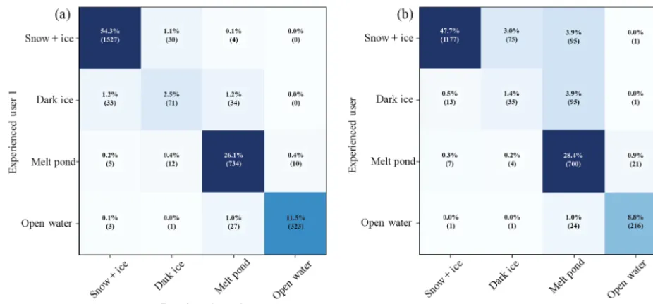
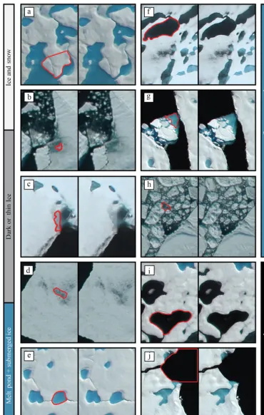
Four training datasets were created to analyze the images se-lected for this paper. One training set was created for each imagery source: panchromatic satellite imagery, multispec-tral satellite imagery, aerial sRGB imagery, and IceBridge DMS imagery. Each training set consists of a list of image objects that have been manually classified by a human and a list of attribute values calculated from those objects and their surroundings. The manual classification is carried out by multiple sea ice experts. Experienced observers of sea ice can classify the majority (85 %+)of segments in a high-resolution optical image with confidence. To address the am-biguity in correct identification of certain segments, however, we used several (4) skilled sea ice observers to repeatedly classify image objects. For the initial creation of our train-ing datasets, two of the users had extensive traintrain-ing in the OSSP algorithm and surface type definitions, while the other two had no experience with the algorithm. Users in both cat-egories were briefed on the standard surface type definitions used for this study (Sect. 3.3.2). Figure 4 shows a confusion matrix to compare user classifications. Cells in the diagonal indicate agreement between users, while off-diagonal cells indicate disagreement (Pedregosa et al., 2011). Agreement between the two well-trained users was high (average 94 % of segment identifications; Fig. 4a), while the agreement be-tween a well-trained user and a new user was lower (average of 86 %; Fig. 4b). After an in-person review of the training objects among all four users, the overall agreement rose to 97 %. The remaining 3 % of objects were cases where the expert users could not agree on a single classification, even after review of the surface type definitions and discussion. These objects were therefore not used in the final training set. Figure 5 shows a series of surface types that span all our classification categories, including those where the classifi-cation is clear and those where it is difficult. Difficult seg-ments are over-represented in these images for illustrative purposes, and represent a relatively small fraction of the total surface.
Figure 4.Confusion matrices comparing classification tendencies between two users experienced with the image processing algorithm(a)
and between an experienced user and a new user(b). Squares are colored based on the value of the cell, with darker colors indicating more matches. Values along the diagonal of each confusion matrix represent the agreement between each user, while values in off-diagonal regions represent disagreement.
creating large training sets is time consuming. We found that training datasets of approximately 1000 points yielded accu-rate and consistent results. We have developed a graphical user interface (GUI) to facilitate the rapid creation of large training sets (see Fig. 6). The GUI presents a user with the original image side by side with an overlay of a single seg-ment on that image. The user assigns a classification to the segment by visual determination.
The training dataset is a critical component of our algo-rithm because it directly controls the accuracy of the machine learning algorithm – and using a consistent training set is necessary for producing intercomparable results. In coordi-nation with this publication we are releasing our version 1.0 training datasets with the intention that they would represent a first version ofthestandard training set to use with each im-age type. Though we have found this training dataset robust through our error analyses below, it is our intention to solicit broader input from the community to refine and expand the training datasets available and release future improved ver-sions.
In addition to cross-validating the creation of a training dataset between users, we assess the quality of our training set through an out-of-bag (OOB) estimate, which is an inter-nal measure of the training set’s predictive power. The ran-dom forest method creates an ensemble (forest) of classifi-cation trees from the input training set. Each classificlassifi-cation tree in this forest is built using a random bootstrap sample of the data in the training set. Because training samples are se-lected at random, each tree is built with an incomplete set of the original data. For every sample in the original training set,
there then exists a subset of classifiers that do not contain that sample. The error rate of each classifier when used to predict the samples that were left out is called the OOB estimate (Breiman, 2001). The OOB estimate has been shown to be equivalent to predicting a separate set of features and com-paring the output to a known classification (Breiman, 1996).
3.5 Assigning classifications
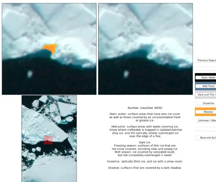
Figure 6.Graphical user interface used to create training datasets and to assess the accuracy of a classified image. Bottom left panel shows an overview of the region to provide the user with spatial context. Top left magnifies the image and highlights the segment of interest, while top right shows the same region with no segment overlap. The user is allowed to choose between any of the relevant surface categories, or to indicate that they are unsure of the classification. As shown, the user interface is demonstrating the classification of a segment for use in a training set. This same GUI is also capable of asking a user to classify an individual pixel, which can be compared to the final classified image for determining accuracy (Sect. 3.6).
area covered by ice floes, i.e.,
Melt pond coverage= AreaMPS AreaMPS+AreaI+S
, (2)
where the subscript MPS indicates predicted melt ponds and submerged ice and I+S indicates predicted ice and snow. 3.6 Determining classification accuracy
The primary measure of classification accuracy was to test the processed imagery on a per pixel basis against human classification. For every processed image, we selected a sple random samsple of 100 pixels chosen from the whole im-age and asked four sea ice experts to assign a classification to those pixels. For a single image from each image source we also asked the sea ice experts to classify and additional
4 Results
4.1 Classification of four imagery sources
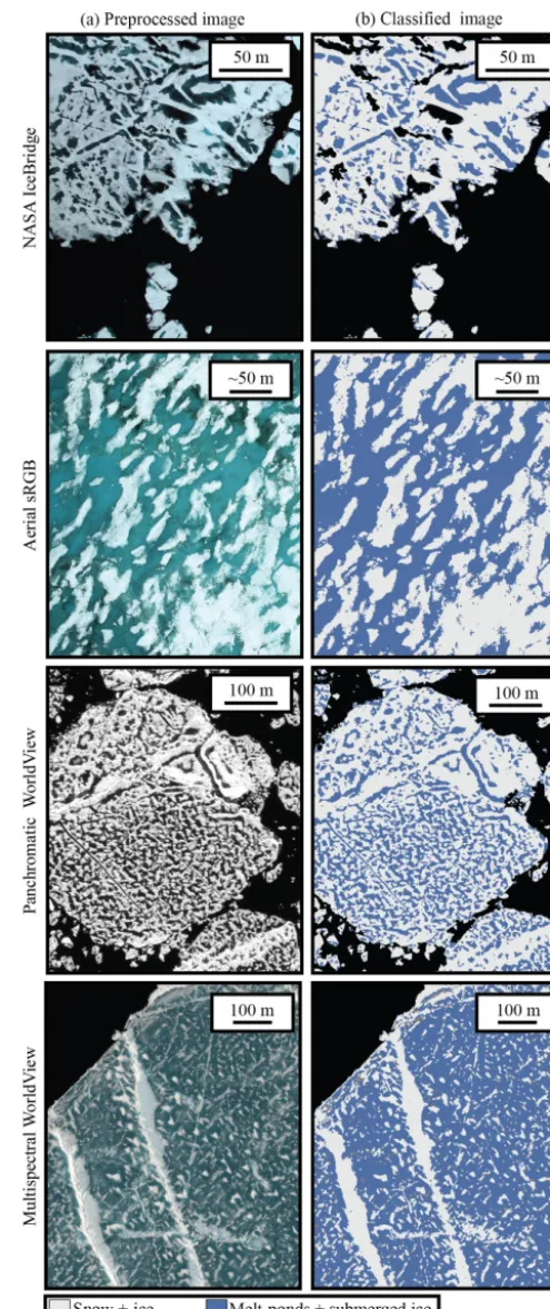
The OSSP image processing method proved highly suitable for the task of classifying sea ice imagery. A visual compari-son between the raw and processed imagery, shown in Fig. 7 can quickly demonstrate this in a qualitative sense. Figure 7 contains a comparison between the original and classified imagery for each source, selected to show the performance of the algorithm on images that contain a variety of surface types. The colors shown correspond to the classification cat-egory; regions colored black are open water, blue regions are melt ponds and submerged ice, gray regions are wet and thin ice, and white regions are snow and ice. The quantitative pro-cessing results, including surface distributions and classifica-tion accuracy, are shown in Table 2. The overall classificaclassifica-tion accuracy was 96±3 % across 20 IceBridge DMS images; 95±3 % across 20 aerial sRGB images; 97±2 % across 22 panchromatic WorldView 1 and 2 images; and 98±2 % across 4 multispectral WorldView 2 images.
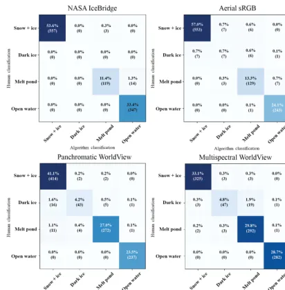
The nature of the classification error is presented using a confusion matrix that compares the algorithm classification with a manual classification for 1000 randomly selected pix-els. Four confusion matrices, one for a single image from each of the four image sources, are shown in Fig. 8. Val-ues along the diagonal of the square are the classifications where the algorithm and the human observer agreed, while values in off-diagonal areas indicate disagreement. Concen-tration of error into a particular off-diagonal cell helps illus-trate the types of confusion the algorithm experiences. The number of pixels that fall into off-diagonal cells is low across all imagery types. In the IceBridge imagery, there is a slight tendency for the algorithm to classify surfaces as open water where a human would choose melt pond. This is caused by exceptionally dark melt ponds on the edge of melting through (Fig. 5f and i). Classification of multispectral WorldView im-agery has a small bias towards classifying melt ponds over dark or thin ice (Fig. 5d). Aerial sRGB and panchromatic WorldView images do not have a distinct pattern to their clas-sification errors.
The internal metric of classification training dataset strength, the OOB estimates, on a 0.0 to 1.0 scale, is shown in Table 3 for the trees built from our four training sets. The OOB estimate represents the mean prediction error of the random forest classifier; i.e., an OOB score of 0.92 estimates that the decision tree would predict 92 % of segments that are contained in the training dataset correctly. The discrepancy between OOB error and the overall classification accuracy is a result of more frequent misclassification of smaller ob-jects; overall accuracy is area weighted, while the OOB score is not.
4.2 WorldView: analyzing a full seasonal progression We analyzed 22 images at a single site in the Beaufort Sea collected between March and August 2014 to challenge the method with images that span the seasonal evolution of ice surface conditions. The site is Eulerian; it observes a sin-gle location in space rather than following a sinsin-gle ice floe through its life cycle as it drifts. Still, the results of these image classifications (shown in Fig. 9) illustrate the progres-sion of the ice surface conditions in terms of our four cate-gories over the course of a single melt season. While cloud cover impacted the temporal continuity of satellite images collected at this site, we are still able to follow the seasonal evolution of surface features. A time series of fractional melt pond coverage calculated from the satellite image site is plot-ted in Fig. 10. The melt pond coverage jumps to 31 % in the earliest June image, as initial ponding begins and floods the surface of the level first year ice. This is followed by a fur-ther increase to 52 % coverage in the next few days. The melt pond coverage then drops back down to 34 % as melt wa-ter drains from the surface and forms well-defined ponds. The evolution of melt pond coverage over our satellite ob-servation period is consistent with prior field obob-servations (Eicken, 2002; Landy et al., 2014; Polashenski et al., 2012) and matches the four stages of ice melt first described by Eicken (2002). The ice at this observation site fully transi-tions to open water by mid-July, though it appears that the ice is advected out of the region in the late stages of melt rather than completing melt at this location.
5 Discussion 5.1 Error
There are four primary sources of error in the OSSP method as presented, two internal to the method and two external. In-ternal error is caused by segment misclassification and by in-complete segmentation (i.e., leaving pixels representing two surface types within one segment). The net internal error was quantified in Sects. 3.6 and 4. External error is introduced by pixilation – or blurring of real surface boundaries due to in-sufficient image resolution – and human error in assigning a “ground truth” value to an aerial or satellite observation dur-ing traindur-ing.
5.1.1 Internal error
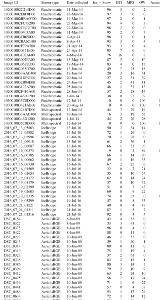
Table 2.The complete results of imagery processed for this analysis. Descriptions for each image include the image type, date collected, the percent of the image that falls into each of the four categories, and the accuracy assessment.
Image ID Sensor type Date collected Ice+Snow DTI MPS OW Accuracy
102001002C214D00 Panchromatic 11-Mar-14 96 3 0 2 97
103001002E8F0D00 Panchromatic 18-Mar-14 97 3 0 0 97
102001002BBA0C00 Panchromatic 19-Mar-14 97 2 0 1 96
103001002FC75200 Panchromatic 23-Mar-14 94 4 0 3 95
102001002CB77C00 Panchromatic 27-Mar-14 98 2 0 0 100
1030010030403A00 Panchromatic 31-Mar-14 95 2 0 3 98
1030010031B65000 Panchromatic 4-Apr-14 96 3 0 1 99
102001002BA6C100 Panchromatic 8-Apr-14 93 3 0 4 100
103001002F79A700 Panchromatic 21-Apr-14 93 3 0 4 98
1030010030371B00 Panchromatic 24-Apr-14 93 7 0 0 98
103001003102A600 Panchromatic 4-May-14 76 16 0 8 98
102001003007FA00 Panchromatic 13-May-14 87 3 0 10 97
10300100306F2E00 Panchromatic 19-May-14 83 4 0 13 96
102001003035D700 Panchromatic 13-Jun-14 49 7 25 18 95
1030010033AAC400 Panchromatic 19-Jun-14 20 3 16 61 97
1020010031DF9E00 Panchromatic 20-Jun-14 27 2 31 39 96
1020010032B94E00 Panchromatic 24-Jun-14 45 2 41 11 95
102001003122A700 Panchromatic 25-Jun-14 48 1 37 13 97
102001002F4F1A00 Panchromatic 28-Jun-14 57 2 28 14 95
10300100346D1200 Panchromatic 1-Jul-14 38 0 23 39 97
1030010035C8D000 Panchromatic 12-Jul-14 0 0 0 100 100
103001003421AB00 Panchromatic 20-Aug-14 0 0 0 100 100
10300100324B7D00 Multispectral 13-Jun-14 44 7 29 19 96
1030010033AAC400 Multispectral 19-Jun-14 16 3 19 62 97
10300100346D1200 Multispectral 1-Jul-14 44 2 26 28 98
1030010035C8D000 Multispectral 12-Jul-14 0 0 0 100 100
2016_07_13_05863 IceBridge 13-Jul-16 50 2 34 14 92
2016_07_13_05882 IceBridge 13-Jul-16 72 1 26 0 97
2016_07_13_05996 IceBridge 13-Jul-16 70 2 28 0 95
2016_07_13_06018 IceBridge 13-Jul-16 61 2 36 1 91
2016_07_13_06087 IceBridge 13-Jul-16 66 1 33 0 99
2016_07_16_00373 IceBridge 16-Jul-16 9 0 2 89 100
2016_07_16_00385 IceBridge 16-Jul-16 66 1 14 20 98
2016_07_16_00662 IceBridge 16-Jul-16 49 1 16 35 98
2016_07_16_00739 IceBridge 16-Jul-16 67 2 25 6 97
2016_07_16_01569 IceBridge 16-Jul-16 22 0 7 71 97
2016_07_16_02654 IceBridge 16-Jul-16 35 0 10 54 95
2016_07_19_01172 IceBridge 19-Jul-16 62 0 14 24 90
2016_07_19_01179 IceBridge 19-Jul-16 57 0 10 32 95
2016_07_19_02599 IceBridge 19-Jul-16 51 0 7 43 99
2016_07_19_02603 IceBridge 19-Jul-16 69 0 9 22 99
2016_07_19_02735 IceBridge 19-Jul-16 74 0 25 0 100
2016_07_19_03299 IceBridge 19-Jul-16 57 0 8 35 96
2016_07_21_01221 IceBridge 21-Jul-16 49 0 4 47 97
2016_07_21_01311 IceBridge 21-Jul-16 87 1 5 7 95
2016_07_21_01316 IceBridge 21-Jul-16 92 0 4 4 99
DSC_0154 Aerial sRGB 8-Jun-09 43 4 53 0 94
DSC_0327 Aerial sRGB 8-Jun-09 33 3 63 0 90
DSC_0375 Aerial sRGB 8-Jun-09 96 0 4 0 99
DSC_0422 Aerial sRGB 8-Jun-09 88 0 11 0 98
DSC_0223 Aerial sRGB 10-Jun-09 46 1 53 0 93
DSC_0243 Aerial sRGB 10-Jun-09 59 1 40 1 98
DSC_0314 Aerial sRGB 10-Jun-09 89 0 11 0 95
DSC_0319 Aerial sRGB 10-Jun-09 75 2 19 4 88
DSC_0323 Aerial sRGB 10-Jun-09 37 2 61 0 95
DSC_0338 Aerial sRGB 10-Jun-09 83 2 15 1 95
DSC_0386 Aerial sRGB 10-Jun-09 80 3 14 3 89
DSC_0394 Aerial sRGB 10-Jun-09 79 2 10 9 95
DSC_0412 Aerial sRGB 10-Jun-09 63 2 24 10 92
DSC_0425 Aerial sRGB 10-Jun-09 56 2 17 24 97
DSC_0439 Aerial sRGB 10-Jun-09 71 1 6 22 98
DSC_0441 Aerial sRGB 10-Jun-09 57 0 4 38 98
DSC_0486 Aerial sRGB 10-Jun-09 53 1 17 29 96
DSC_0634 Aerial sRGB 10-Jun-09 72 1 14 12 96
DSC_0207 Aerial sRGB 13-Jun-09 80 1 19 0 96
Figure 8.Accuracy confusion matrices comparing the classification of 1000 pixels between a human and the algorithm. Squares are colored based on the value of the cell, with darker colors indicating more matches. Values along the diagonal of each confusion matrix represent the agreement between each classifier, while values in off-diagonal regions represent disagreement.
Table 3.Out-of-bag scores for the three training datasets used to classify imagery from each of the four sensor platforms, and the number of objects manually classified for each set.
Image Training dataset Out-of-bag
source size error
Panchromatic WorldView 1000 0.94 Pansharpened WorldView 859 0.89 Aerial imagery 945 0.94 IceBridge imagery 940 0.91
can practically be determined from labor-intensive ground campaign techniques such as lidar and measured linear tran-sects (e.g., Polashenski et al., 2012)
cate-Figure 9.Seasonal progression of surface type distributions at the satellite image collection site; 2014 in the Beaufort Sea at 72◦N, 128◦W. This site represents a Eulerian observation of the sea ice surface and does not track a floe across its lifetime. Average scene size was 956 km2 with a minimum of 304 km2and a maximum of 1321 km2.
gory was the Dark and Thin Ice subcategory of Ice and Snow. This category often represents surface types that are in a tran-sitional state and is often difficult to classify even for a hu-man observer.
The second type of internal error is segmentation error, where an object is created that contains more than one of the surface types we are trying to distinguish. This occurs when boundaries between objects are not placed where boundaries between surfaces exist – an issue most common where one surface type gradually transitions to another. When this oc-curs, some portion of that object will necessarily be mis-classified. We have compensated for areas that lack sharp boundaries by biasing the image segmentation towards over-segmentation, but a small number of objects still contain more than one surface type. During training set creation, we asked the human experts to identify objects containing more than one surface type. In total, 3.5 % of objects were identi-fied as insufficiently segmented in aerial imagery, and 2 % of objects in satellite imagery. This represents the upper limit for the total percentage of insufficiently segmented objects for several reasons. First, segmentation error was most preva-lent in transitional surface types (i.e., Dark and Thin Ice), which represents a small portion of the overall image and is composed of relatively small objects. This category is over-represented in the training objects because objects were cho-sen to sample each surface type and not weighted by area. In addition, insufficiently segmented objects are generally com-posed of only two surface types and end up identified as the surface which represents more of the object’s area. Hence the total internal error introduced by segmentation error is appre-ciably smaller than misclassification error, likely well under 1 %.
5.1.2 External error
The first form of external error is introduced by image reso-lution. At lower image resolutions, more pixels of the image span edges, and smaller features are more likely to go unde-tected. Pixels on the edge of surface types necessarily
repre-Date
01 May 01 Jun 01 Jul
Melt pond fraction (%) 0
20 40 60 80 100
Figure 10.Evolution of melt pond fraction over the 2014 season at our satellite image collection site; 2014 in the Beaufort Sea at 72◦N, 128◦W. This site represents a Eulerian observation of the sea ice surface, and does not track a floe across its lifetime. By August, the sea ice extent has retreated north of this location, and we therefore do not capture a full melt pond cycle.
sent more than one surface type, but can be classified as only one. Misclassification of these has the potential to become a systemic error if edge pixels were preferentially placed in a particular category. We assessed this error’s impact by taking high-resolution IceBridge imagery (0.1 m), downsampling to progressively lower resolution, and reprocessing. Figure 11 shows the surface type percentages for three IceBridge im-ages at decreasing resolution. Figure 12 shows a series of downsampled images and their classified counterparts. Sur-prisingly, despite clear pixilation and aliasing in the imagery, little change in aggregate classification statistics occurred as resolution was lowered from 0.1 to 2 m. This suggests that at resolutions used for this paper, edge pixels do not sig-nificantly impact the classification results. It may also be possible to forego the pansharpening process discussed in Sect. 3.1 and use 2 m multispectral WorldView imagery di-rectly.
Figure 11. Change in surface coverage percentage as a result of downsampling three IceBridge images. Each plot represents a single image, with resolution along thexaxis on a log scale. Imagery starts at the nominal IceBridge resolution of 0.1 m and is degraded to a maximum of 50 m.
Figure 12.Visual demonstration of the downsampling effect on a single NASA IceBridge image. The top image is shown at the orig-inal 0.1 m resolution. The middle image is a resolution of 2 m – the equivalent of a multispectral WorldView 2 image without pan-sharpening. The bottom has a resolution of 10 m, where pixel size has begun to exceed the average melt pond size.
3 % of objects creating our training sets. The possibility of systemic bias among the expert observer classifications can-not be excluded because real ground truth, in the form of geo-referenced ground observations from knowledgeable ob-servers was, unfortunately, not available for any of the im-agery. Conducting this type of validation would be helpful, but given high confidence human expert classifiers expressed in their classifications and low disagreement between them, it may not be essential.
5.1.3 Overall error
The fact that misclassification dominates the internal error metric suggests that error could be reduced if additional ob-ject attributes used by human experts to differentiate surface types could be identified. The agreement between the OSSP method and a human (96 %±3 %) is similar to the agree-ment between different human observers (97 %), meaning that the algorithm is nearly as accurate as a human manu-ally classifying an entire image. If we exclude the possibility for systemic error in human classification, and assume other errors are unrelated to one another, we can calculate a total absolute accuracy in surface type determination as approxi-mately 96 %.
5.2 Producing derived metrics of surface coverage The classified imagery, presented as a raster (e.g., Fig. 7), is not likely to be the end product used in many analyses. Met-rics of the sea ice state in simpler form will be calculated. We already introduced the most basic summary metrics in Sect. 4, where we presented fractional surface coverage cal-culated from the total pixel counts for each of the four surface categories in each image. We also presented the calculation of melt pond coverage as a fraction of the ice-covered por-tion of the image, rather than total image area. The calcu-lation of these is straightforward. Other metrics commonly discussed in the literature that could be produced with mini-mal additional processing include those capturing melt pond size, connectivity, or fractal dimension, as well as floe size distribution or perimeter-to-area ratio. As with definitions of surface type, standardizing metrics will be necessary to pro-duce intercomparable results. We discussed the more com-plex metrics which could be derived from this imagery with several other groups. We determined that standardizing these and other more advanced metrics will require more input and consensus building before a community standard can be sug-gested. We leave determining standard methods for calculat-ing these more complex metrics to a future work.
Equipped with the images processed by OSSP, we con-sider what size area must be imaged, classified, and sum-marized to constitute “one observation” and how regionally representative such an observation is. Even with the increas-ing availability of high-resolution imagery, it is unlikely that high-resolution imaging will regularly cover more than a
small portion of the Arctic in the near future. As a result, high-resolution image analysis will likely remain a “sam-pling” technique. Since the scale of sea ice heterogeneity varies for each property type, a minimum area unique to that property must be analyzed to qualify as a representa-tive sample of the surface conditions. Finding that minimum area involves addressing the “aggregate scale” – the area over which a measured surface characteristic becomes uniform and captures a representative average of the property in the area (Perovich, 2005). It may also be possible to determine an aggregate-scale statistic within well-constrained bounds by random sub-sampling of the region and therefore reduce processing time. Here we conduct analysis of these sampling concepts and suggest this analysis of the aggregate scale be conducted for any metric.
First, we sought to determine the aggregate scale for the simple fractional coverage metrics of ice as a fraction of to-tal area and melt pond as a fraction of ice area. This would inform us, for example, as to whether processing the en-tire area of a WorldView image (up to 1000 km2)was nec-essary, or alternatively if a full WorldView image was suf-ficient to constitute a sample. First, we evaluated the con-vergence of fractional coverage within areas of increasing size towards the image mean. For a WorldView image de-picting primarily first year ice in various stages of melt, we created non-overlapping gridded subsections and determined the fractional coverage within each grid cell. The size of grid cells was varied logarithmically from 100×100 pixels (102)
see that the range of the prediction interval generally drops as larger samples are taken, but it does not converge as cleanly or quickly as the pond coverage prediction interval does – a finding that is unsurprising as ice fraction is composed of discrete floes with sizes much larger than melt ponds. The limited convergence indicates that the aggregate scale for de-termination of ice covered fraction is at least on the order of the scale of a WorldView image, and likely larger. Aggregate scale ice concentration, unlike melt pond fraction, is a statis-tic better observed with medium resolution remote sensing platforms such as MODIS or Landsat due to the need for a larger satellite footprint. WorldView imagery may be partic-ularly useful for determining smaller-scale parts of floe size distributions or for validating larger-scale remote sensing of ice fraction, if the larger-scale pixels can be completely con-tained within the WorldView image. Floe size distribution will likely require nesting of scales in order to fully access both large- and small-scale parts of the floe size distribution. We next investigated whether it is possible to reduce the processing load required to determine the melt pond or ice fraction of an image within certain error bounds by process-ing collections of random image subsets. To do this, it is use-ful to first establish two definitions: (1) one random sample of size N representsN randomly selected 100×100 pixel boxes, and (2) one adjacent sample of size N is a single area with size 100
√
N ×100
√
N. In other words, a ran-dom sample and an adjacent sample both represent an im-age area of 10 000·N pixels, but consist of independent and correlated pixels, respectively. We expect random samples to better represent the total image mean melt pond fraction because ice conditions are spatially correlated and a single large area is not composed of independent samples. We eval-uated this hypothesis by collecting 1000 random and adja-cent samples of sizeN=100, with replacement. Results are shown in Fig. 14. In Fig. 14a, we plot a histogram of the mean melt pond fraction determined from these 1000 samples. The means determined from sets that contained randomly dis-tributed image areas, are in red. The means determined from sets of adjacent image areas are in blue. Although both sets represent samples of the same total image area, the one com-posed of independent subsets randomly selected from across the image does a much better job of representing the mean value, with a smaller standard deviation.
Estimating the mean of a complete image by sampling ran-domly selected areas of the image becomes a simple statistics problem. The sample size needed to estimate a population mean to within a certain confidence interval and margin of error can be determined with the formula
n=
Zσ
ME 2
, (3)
wheren is the sample size, Z is thezscore for the confi-dence interval required,σ is the population standard devia-tion, and ME is the margin of error. The standard deviation of 1000 random samples with size 100 (Fig. 14a) is∼0.05. The
Figure 13. Convergence of melt pond fraction(a)and ice frac-tion(b)for a WorldView image collected on 25 June 2014 at 72◦N, 128◦W as the area evaluated is increased. Small blue dots represent individual image subsets. For segments of a given size, black dots represent the mean value of those samples, red dots represent the 95 % prediction interval, and purple dots show the 95 % prediction interval for the same total area, but calculated from 100 randomly placed, smaller, samples. Cyan shaded area represents the error in determination expected from the processing method.
Figure 14.Histogram of melt pond fraction(a)and ice fraction(b)for 1000 samples, where each sample is the mean surface fraction within 100, 50 m by 50 m, squares. The 100 squares were either randomly distributed across the image (red) or adjacent to each other (blue). Calculated from a 25 June 2014 WorldView image.
±4 %, with 95 % confidence. A total of 38 samples of size 100 corresponds to an image area of∼10 km2, significantly smaller than the total image size.
In order to show these results visually, we return to Fig. 13 and place another set of 95 % prediction interval bounds (pur-ple dots). These bounds represent the prediction interval for a random sample of size necessary for the total area to equal the area on thex axis. The result is quite powerful. By pro-cessing as little as 10 km2of the image, collected from sam-ples randomly distributed across the area, we can determine aggregate melt pond fraction to within 4 % of the true value with a confidence of 95 %. For large-scale processing we suggest that when the sample confidence interval is below the image processing technique accuracy, sampling of larger areas is no longer necessary.
A similar analysis is presented in Figs. 13b and 14b for ice fraction. While the WorldView image is likely not large enough to represent the aggregate scale for ice fraction, ran-domly sampling the image still provides an expedient way to determine the mean ice fraction of the image within certain bounds, while processing only a small fraction of the image. Calculating the 95 % prediction interval of random samples representing the total image area shown on thexaxis (purple dots) again shows that the total image mean can be estimated by calculating only a small portion of the total image.
These explorations of image sampling permit us to recom-mend that users can estimate the total image pond fraction
5.3 Community adoption
We have provided a free distribution of the OSSP algo-rithm and the training sets discussed in Sects. 3.4 and 4 as a companion to this publication, complete with de-tailed startup guides and documentation. This OSSP algo-rithm has been implemented entirely in Python using open-source reopen-sources with release to additional users in mind. The code, along with documentation, instructional guide-lines, and premade training sets (those used for the anal-yses herein) is available at https://github.com/wrightni/ossp (https://doi.org/10.5281/zenodo.1133689). The software is packaged with default parameters and version-controlled training sets for four different imagery sources. The pack-age includes a graphical user interface to allow users to build custom training datasets that suit their individual needs. The algorithm was constructed with the flexibility to allow for the classification of any number of features given an appropriate training dataset.
Our intention is that by providing easy access to the code in an open-source format, we will enable both specific in-quiries and larger-scale image processing that supports com-munity efforts at general sea ice monitoring. We plan to con-tinue improving and updating the code as it gains users and we receive community feedback. We hope to encourage oth-ers to design their own features and add-ons. Since the pre-dictive ability of the machine learning algorithm improves as more training data are added, we wish to strongly encourage the use of the GUI to produce additional training sets and we plan to collate other users training sets into improved train-ing versions. See documentation of the traintrain-ing set creation GUI for more information on how to share a training set.
The OSSP algorithm helps to bring the goal of having a standardized method for deriving geophysical parameters from high-resolution optical sea ice imagery closer to real-ity. In the larger picture, developing such a tool is only the first step. We recall that the motivation behind this develop-ment was the need to quantify sea ice surface conditions in a way that could enable better understanding of the processes driving changes in sea ice cover. The value of the toolkit will only be realized if it is used for these scientific inquiries. We look forward to working with imagery owners to facilitate processing of additional datasets.
6 Conclusions
We have implemented a method for classifying the sea ice surface conditions from high-resolution optical imagery of sea ice. We designed the system to have a low barrier to en-try, by coding it in an open-source format, providing detailed documentation, and releasing it publicly for community use. The code identifies the dominant surface types found in sea ice imagery (open water, melt ponds and submerged ice, and snow and ice) with accuracy that averages 96 % – comparable
to the consistency between manual expert human classifica-tions of the imagery. The algorithm is shown to be capable of classifying imagery from a range of image sensing platforms including panchromatic and pansharpened WorldView satel-lite imagery, aerial sRGB imagery, and optical DMS imagery from NASA IceBridge missions. Furthermore, the software can process imagery collected across the seasonal evolution of the sea ice from early spring through complete ice melt, demonstrating it is robust even as the characteristics of the ice features seasonally evolve. We conclude, based on our error analysis, that this automatic image processing method can be used with confidence in analyzing the melt pond evo-lution at remote sites.
With appropriate processing, high-resolution imagery col-lections should be a powerful tool for standardized and rou-tine observation of sea ice surface characteristics. We hope that in providing easy access to the methods and algorithm developed herein, we will facilitate the sea ice community’s convergence on a standardized method for processing high-resolution optical imagery either by adoption of this method or by suggestion of an alternate method complete with code release and error analysis.
Data availability. The OSSP algorithm code is available from https://github.com/wrightni/ossp (https://doi.org/10.5281/zenodo.1133689; Wright, 2017). Im-age data and processing results are available at the NSF Arctic Data Center (ADC). Raw and preprocessed image data from DigitalGlobe WorldView images are not available due to copyright, but can be acquired from DigitalGlobe or the Polar Geospatial Center at the University of Minnesota.
Competing interests. The authors declare that they have no conflict of interest.
Acknowledgements. This work was supported by the Office of Naval Research Award N0001413MP20144 and the National Science Foundation Award PLR-1417436. We would like to thank Donald Perovich and Alexandra Arntsen for their assis-tance in creating machine learning training datasets. We would also like to thank Arnold Song, Justin Chen, and Elias Deeb for their assistance and guidance with the development of the OSSP code. WorldView satellite imagery was provided with the DigitalGlobe NextView License through the University of Minnesota Polar Geospatial Center. A collection of the aerial imagery was collected by the SIZONet project. Some data used in this paper were acquired by the NASA Operation IceBridge Project. Edited by: Bert Wouters
References
Arntsen, A. E., Song, A. J., Perovich, D. K., and Richter-Menge, J. A.: Observations of the summer breakup of an Arctic sea ice cover, Geophys. Res. Lett., 42, 8057–8063, https://doi.org/10.1002/2015GL065224, 2015.
Blaschke, T.: Object based image analysis for remote sens-ing, ISPRS J. Photogramm. Remote Sens., 65, 2–16, https://doi.org/10.1016/j.isprsjprs.2009.06.004, 2010.
Blaschke, T., Hay, G. J., Kelly, M., Lang, S., Hofmann, P., Addink, E., Queiroz Feitosa, R., van der Meer, F., van der Werff, H., van Coillie, F., and Tiede, D.: Ge-ographic Object-Based Image Analysis – Towards a new paradigm, ISPRS J. Photogramm. Remote Sens., 87, 180–191, https://doi.org/10.1016/j.isprsjprs.2013.09.014, 2014.
Breiman, L.: Bagging Predictors, Mach. Learn., 24, 123–140, https://doi.org/10.1023/A:1018054314350, 1996.
Breiman, L.: Random Forests, Mach. Learn., 45, 5–32, https://doi.org/10.1023/A:1010933404324, 2001.
Curry, J. A., Schramm, J. L., and Ebert, E. E.: Sea ice-albedo climate feedback mechanism, J. Cli-mate, 8, 240–247, https://doi.org/10.1175/1520-0442(1995)008<0240:SIACFM>2.0.CO;2, 1995.
DeFries, R.: Multiple Criteria for Evaluating Machine Learn-ing Algorithms for Land Cover Classification from Satellite Data, Remote Sens. Environ., 74, 503–515, https://doi.org/10.1016/S0034-4257(00)00142-5, 2000. DeMott, P. J. and Hill, T. C. J.: Investigations of Spatial and
Tem-poral Variability of Ocean and Ice Conditions in and Near the Marginal Ice Zone, The “Marginal Ice Zone Observations and Processes Experiment” (MIZOPEX) Final Campaign Summary, DOE ARM Climate Research Facility, Pacific Northwest Na-tional Laboratory, Richland, Washington, 2016.
Dominguez, R.: IceBridge DMS L0 Raw Imagery, Version 1, https://doi.org/10.5067/UMFN22VHGGMH, 2010.
Duro, D. C., Franklin, S. E., and Dubé, M. G.: A comparison of pixel-based and object-based image analysis with selected ma-chine learning algorithms for the classification of agricultural landscapes using SPOT-5 HRG imagery, Remote Sens. Environ., 118, 259–272, https://doi.org/10.1016/j.rse.2011.11.020, 2012. Eicken, H.: Tracer studies of pathways and rates of meltwater
trans-port through Arctic summer sea ice, J. Geophys. Res., 107, 8046, https://doi.org/10.1029/2000JC000583, 2002.
Fetterer, F. and Untersteiner, N.: Observations of melt ponds on Arctic sea ice, J. Geophys. Res.-Oceans, 103, 24821–24835, https://doi.org/10.1029/98JC02034, 1998.
GDAL: GDAL – Geospatial Data Abstraction Library, Version 2.1.0, Open Source Geospatial Found, available at: http://gdal. org (last access: 17 July 2017), 2016.
Inoue, J., Curry, J. A., and Maslanik, J. A.: Applica-tion of Aerosondes to Melt-Pond Observations over Arctic Sea Ice, J. Atmos. Ocean. Tech., 25, 327–334, https://doi.org/10.1175/2007JTECHA955.1, 2008.
Kurtz, N. T., Farrell, S. L., Studinger, M., Galin, N., Harbeck, J. P., Lindsay, R., Onana, V. D., Panzer, B., and Sonntag, J. G.: Sea ice thickness, freeboard, and snow depth products from Oper-ation IceBridge airborne data, The Cryosphere, 7, 1035–1056, https://doi.org/10.5194/tc-7-1035-2013, 2013.
Kwok, R.: Declassified high-resolution visible imagery for Arctic sea ice investigations: An overview, Remote Sens. Environ., 142, 44–56, https://doi.org/10.1016/j.rse.2013.11.015, 2014. Kwok, R. and Rothrock, D. A.: Decline in Arctic sea ice thickness
from submarine and ICESat records: 1958–2008, Geophys. Res. Lett., 36, L15501, https://doi.org/10.1029/2009GL039035, 2009. Landy, J., Ehn, J., Shields, M., and Barber, D.: Surface and melt pond evolution on landfast first-year sea ice in the Canadian Arctic Archipelago, J. Geophys. Res.-Oceans, 119, 3054–3075, https://doi.org/10.1002/2013JC009617, 2014.
Laxon, S. W., Giles, K. A., Ridout, A. L., Wingham, D. J., Willatt, R., Cullen, R., Kwok, R., Schweiger, A., Zhang, J., Haas, C., Hendricks, S., Krishfield, R., Kurtz, N., Far-rell, S., and Davidson, M.: CryoSat-2 estimates of Arctic sea ice thickness and volume, Geophys. Res. Lett., 40, 732–737, https://doi.org/10.1002/grl.50193, 2013.
Lu, P., Li, Z., Cheng, B., Lei, R., and Zhang, R.: Sea ice surface features in Arctic summer 2008: Aerial observations, Remote Sens. Environ., 114, 693–699, https://doi.org/10.1016/j.rse.2009.11.009, 2010.
Markus, T., Cavalieri, D. J., Tschudi, M. A., and Ivanoff, A.: Comparison of aerial video and Landsat 7 data over ponded sea ice, Remote Sens. Environ., 86, 458–469, https://doi.org/10.1016/S0034-4257(03)00124-X, 2003. Markus, T., Stroeve, J. C., and Miller, J.: Recent changes in Arctic
sea ice melt onset, freezeup, and melt season length, J. Geophys. Res., 114, C12024, https://doi.org/10.1029/2009JC005436, 2009.
Maslanik, J., Stroeve, J., Fowler, C., and Emery, W.: Distribution and trends in Arctic sea ice age through spring 2011, Geophys. Res. Lett., 38, L13502, https://doi.org/10.1029/2011GL047735, 2011.
Miao, X., Xie, H., Ackley, S. F., Perovich, D. K., and Ke, C.: Object-based detection of Arctic sea ice and melt ponds using high spa-tial resolution aerial photographs, Cold Reg. Sci. Technol., 119, 211–222, https://doi.org/10.1016/j.coldregions.2015.06.014, 2015.
Miao, X., Xie, H., Ackley, S. F., and Zheng, S.: Object-Based Arctic Sea Ice Ridge Detection From High-Spatial-Resolution Imagery, IEEE Geosci. Remote Sens. Lett., 13, 787–791, https://doi.org/10.1109/LGRS.2016.2544861, 2016.
Pal, M.: Random forest classifier for remote sensing classification, Int. J. Remote Sens., 26, 217–222, https://doi.org/10.1080/01431160412331269698, 2005. Parkinson, C. L. and Comiso, J. C.: On the 2012 record low
Arctic sea ice cover: Combined impact of preconditioning and an August storm, Geophys. Res. Lett., 40, 1356–1361, https://doi.org/10.1002/grl.50349, 2013.
Pedregosa, F., Varoquaux, G., Gramfort, A., Michel, V., Thirion, B., Grisel, O., Blondel, M., Prettenhofer, P., Weiss, R., Dubourg, V., Vanderplas, J., Passos, A., Cournapeau, D., Brucher, M., Perrot, M., and Duchesnay, É.: Scikit-learn: Machine Learning in Python, J. Mach. Learn. Res., 12, 2825–2830, available at: http://jmlr.csail.mit.edu/papers/v12/pedregosa11a.html (last ac-cess: 24 July 2017), 2011.