www.atmos-meas-tech.net/9/1/2016/ doi:10.5194/amt-9-1-2016
© Author(s) 2016. CC Attribution 3.0 License.
Assessment of adequate quality and collocation of reference
measurements with space-borne hyperspectral infrared instruments
to validate retrievals of temperature and water vapour
X. Calbet
EUMETSAT, Eumetsat Allee 1, 64295 Darmstadt, Germany
Correspondence to: X. Calbet ([email protected]) or ([email protected])
Received: 10 March 2015 – Published in Atmos. Meas. Tech. Discuss.: 5 June 2015 Revised: 16 November 2015 – Accepted: 24 November 2015 – Published: 15 January 2016
Abstract. A method is presented to assess whether a given reference ground-based point observation, typically a ra-diosonde measurement, is adequately collocated and suffi-ciently representative of space-borne hyperspectral infrared instrument measurements. Once this assessment is made, the ground-based data can be used to validate and potentially cal-ibrate, with a high degree of accuracy, the hyperspectral re-trievals of temperature and water vapour.
1 Introduction
Space-borne infrared hyperspectral instruments typically measure Earth views in a spectral range from 600 to 3000 cm−1wavenumbers with a spectral sampling of about 0.25 cm−1providing thousands of channels across their full
spectral range. From these measurements it is possible to re-trieve atmospheric profiles of temperature and water vapour with a relatively high vertical resolution and high degree of accuracy. These (so-called) retrievals can have a temperature accuracy of about 1 K in layers 1 km thick and humidity ac-curacy from 10 to 20 % in layers 2 km thick within the tro-posphere (Smith et al., 2001). The algorithms to obtain these retrievals are usually of the following two kinds.
– Regression methods – These are methods based on re-gression techniques like artificial neural networks, ker-nel ridge regression or, more simply, a linear regression (see for example Camps-Valls et al., 2012). These meth-ods are usually trained with a representative sample of atmospheric profiles and their corresponding radiances. This training sample can be obtained either by using
di-rect measurements of both radiances and atmospheric profiles or by simulating the radiances from the atmo-spheric profiles using a radiative transfer model. Radia-tive transfer models simulate the propagation of light in the atmosphere by accepting an atmospheric profile as input and providing radiances as output. The regres-sion methods are later used operationally by providing the measured radiances as input and obtaining the atmo-spheric profiles as output via the regression.
– Minimization methods – The second kind of retrieval algorithms need a radiative transfer model to operate. In these algorithms, the radiances obtained from the ra-diative transfer model are matched to the measured ones by modifying the input atmospheric profiles via a min-imization algorithm until both calculated and measured radiances coincide within a given error. A well known method in this category is “optimal estimation” (OE, Rodgers , 2000).
that might remain between the ground-based reference mea-surement and the satellite one. Other sources of uncertainties can be an incorrect modelling of the radiative transfer or an unexpected behaviour in the noise characteristics of the hy-perspectral instrument.
To effectively take a reference measurement, the error of a particular profile has to be much smaller than the error of its corresponding hyperspectral retrieval. This condition is usually met when hyperspectral retrievals are compared to sondes, which typically have an error of 0.1 K for tempera-ture and at most 3 % for relative humidity in the lower and mid troposphere (Paukkunen et al., 2001; Miloshevich et al., 2006). It is also necessary that the reference measurements are free of bias and have no systematic errors, a circumstance that is not always met when measuring humidity with certain type of sondes which can have up to a 50 % systematic er-ror in the upper troposphere (e.g., Vömel et al., 2007). This effect could render the comparison ineffective.
An added complication is that the reference measurement usually measures a collection of parcels in the atmosphere which are not exactly the same as the ones measured by the hyperspectral instrument. A radiosonde, for example, mea-sures at one small region or point in the atmosphere and it drifts from the launch location, measuring in different loca-tions and at different times, whereas a hyperspectral instru-ment measures nearly instantly a large region of the atmo-sphere with typical footprints of tens of kilometres. These ef-fects contribute to a significant difference between both mea-surements; this amounts to what is called collocation uncer-tainty. A notable example is water vapour, which has a high variability in the atmosphere with very small temporal and spatial scales (Vogelmann et al., 2015), making the colloca-tion particularly difficult. In order for the validacolloca-tion to be ef-fective, the collocation uncertainty needs to be much smaller than the error of its corresponding retrieval (Sussmann et al., 2009; Vogelmann et al., 2011).
There are currently two possible strategies to overcome these problems. One of them is to estimate all the errors involved in the validation process, from reference measure-ment errors to collocation uncertainties plus any other error that could affect the comparison. One such attempt has been done by Pougatchev et al. (2009). Another strategy is to as-sess whether the global measurement, collocation and radia-tive transfer modelling errors are small enough to make the validation useful. This is the objective of this paper, where a method to assess the adequacy of an individual reference measurement to a particular retrieval methodology is pre-sented. Since the method, as will be seen below, is based on comparing the satellite measured radiances with the calcu-lated ones using the radiative transfer model and the refer-ence atmospheric profiles, it only applies to retrieval meth-ods based on a radiative transfer model and it is not directly applicable to other retrieval methods (i.e. regression methods trained with measured data).
To illustrate the method, one spectrum from a single In-frared Atmospheric Sounding Interferometer (IASI) field of view is used and four different IASI collocated potential reference profiles are analysed. These data are described in Sect. 2. The method is described in Sect. 3. Finally, a discus-sion of the method is portrayed in the concludiscus-sions.
2 Data 2.1 Raw data
Infrared hyperspectral data are obtained from the IASI in-strument on board the polar orbiting satellite Metop-A. IASI is measuring within the whole spectral range from 645 to 2760 cm−1 with a spectral sampling of 0.25 cm−1, an apodized effective resolution of 0.25 cm−1 and with a spa-tial resolution of about 12 km at nadir. One single IASI field of view is analyzed in this study over the Sodankylä ob-servatory, northern Finland (location: 67.368◦N, 26.633◦E, 179 m a.s.l.) overpassing the observatory on 17 July 2007 at 08:18 Z. This particular field of view is selected because it is cloud free, making the radiative transfer model calcula-tions simpler. It also has a significant set of accompanying ground-based measurements from the EPS/Metop Sodankylä campaign.
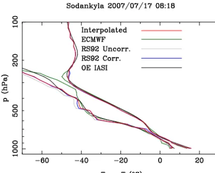
Radiosonde data are from the EPS/Metop Sodankylä cam-paign, which took place during the time period 4 June to 5 September 2007 (for more details see Calbet et al., 2011). Also, ECMWF analyses have been used either on its own or to complement the radiosonde data. The particular reference temperature and water vapour profiles, which are plotted in Fig. 1, are obtained from the following sources.
– Nearest geo-located ECMWF analysis at 06 Z, which is about 2:30 h before satellite overpass time – This profile will be referred to as “ECMWF”.
– Interpolated sonde data from two sonde measurements – A Cryogenic Frost Point Hygrometer (CFH) one, in which the sonde is launched 1 h before satellite over-pass time, and an “in situ” bias corrected RS92 one, in which the sonde is launched 5 min before satellite overpass time. The interpolation is done in the time do-main following Tobin et al. (2006). The “in situ” bias correction is derived from the comparison of the CFH sonde data with the data from yet another RS92 sonde. These latter two sondes are flown on the same balloon launched 1 h before satellite overpass time. This pro-file will be referred to as “Interpolated”. In this paper, it is taken as the best estimate of the atmosphere for this hyperspectral observation. See Calbet et al. (2011) for more details.
Figure 1. Temperature and dew point temperature of the different
profiles used in this paper. The OE IASI retrieval is also shown (in black) for reference purposes only.
following Vömel et al. (2007) and without any kind of interpolation, i.e., using solely data from this RS92 sonde – This data will be referred to as “RS92 Corr.”.
– RS92 sonde launched 5 min before overpass time with-out any kind of bias corrections – This data will be re-ferred to as “RS92 Uncorr.”.
It is now worth looking at the different profiles in Fig. 1. They are generally very similar and consistent ex-cept for a few differences. The water vapour concentration for “ECMWF” is clearly much higher than the other ones in the upper troposphere/low stratosphere. The “RS92 Uncorr.” profile is much drier than the others from mid troposphere up. These differences will show up in the observed minus calculated radiances analysis made below (Figs. 4 and 5).
2.2 IASI retrievals
One IASI retrieval is obtained for comparison purposes. The retrieval also constitutes a good starting point to estimate the OE retrieval error, which is essential for the method pre-sented here, but the error could also be calculated from any other realistic atmospheric profile which matches the situ-ation. The IASI retrieval has been calculated following the techniques described in Calbet et al. (2006) and the fine tun-ing of Calbet (2012). The general description and some par-ticular enhancements and modifications introduced with re-spect to Calbet et al. (2006) are briefly summarized below:
– Retrievals were obtained using optimal estimation (OE) Rodgers (2000) with physical constraints by prohibit-ing supersaturation and superadiabaticity.
– All IASI channels from band 1 and 2 have been used, but excluding the ozone band.
– The background state and matrix used in the OE have been obtained from the Chevallier (2002) data set. – Fine tuning of the OE has been done with collocated
ECMWF analyses Calbet (2012), both with respect to bias corrections and measurement error covariance ma-trix. Due to the significant inaccuracy of ECMWF wa-ter vapour analyses (e.g. quite noticeable in Fig. 1), the resulting measurement error covariance matrix used in OE is clearly overestimated in the water vapour band. This leads to a relatively big expected error in the water vapour retrievals (Fig. 8).
– First guess with which the OE is initialized is the “In-terpolated” profile, which is considered to be the best estimate of the atmosphere for this case.
– Radiative transfer model is the optimal spectral sam-pling (OSS) from Moncet et al. (2008) trained with the Line–By–Line Radiative Transfer Model (LBLRTM) version 11.3.
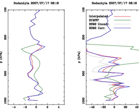
For illustration purposes the differences of these four pro-files against the OE retrieval are plotted in Fig. 2. It can be seen that the differences depend very strongly on the refer-ence profile used. While most profiles do not deviate signif-icantly from the OE retrieval, the “ECMWF” profile does show comparatively large differences. It is worth noting that all the radiosonde data come from the EPS/Metop Sodankylä campaign and therefore has not been assimilated into any Numerical Weather Prediction (NWP) model.
3 Method
The assessment method consists of two steps. In the first one the observed radiances are compared to the calculated ones. The second step consists in converting the mentioned radi-ance differences into atmospheric state differences.
3.1 Observed minus calculated radiances
To get a sense of how well the reference atmospheric profiles are representative of the atmosphere at the IASI field of view, the IASI measured radiances can be compared to the calcu-lated ones using a radiative transfer model. This effectively means that the measured atmospheric profile, the radiative transfer model and the IASI radiances are consistent among themselves within their measurement errors.
Figure 2. Difference of the reference profiles minus the OE
re-trieval.
measurements, like they would be if a retrieval is performed or some other similar kind of technique is used. The reason behind this is that the final goal of the study is to make an assessment of the reference profile and not of the retrieval. Using data obtained from IASI radiances would artificially increase the agreement between the calculated and measured radiances, thus affecting our assessment method. In the most extreme case, when using atmospheric profiles and quantities that are all derived or retrieved from IASI radiances, it is the retrieval that is assessed and not the reference profiles. It is not always possible to meet this requirement in practice, and it is often the case that some of the parameters needed as in-put for the radiative transfer model are missing, as typically happens with surface emissivity or surface skin temperature. If this is the case, the number of retrieved parameters should be minimized as much as possible.
In particular, in this paper the calculated radiances are ob-tained using the following methods.
– The temperature and water vapour profiles are used based on radiosonde measurements (“Interpolated”, “RS92 Corr.” and “RS92 Uncorr.”), which are comple-mented in the upper layers, where the sonde instruments reach their limit, with the “ECMWF” profile. See Calbet et al. (2011) for more details.
– The ozone profile is obtained from the ECMWF analy-sis for all cases.
– The radiative transfer model used is OSS Moncet et al. (2008), trained with LBLRTM 11.3.
– Surface emissivity is the one corresponding to old pine leaf from the MODIS UCSB emissivity library MODIS Emissivity (1999). This surface emissivity seems to be
Figure 3. IASI observed minus calculated radiances (OBS-CALC)
for the “Interpolated” profile.
the most appropriate for this site, which is covered by an old pine forest.
– Surface skin temperature measurements are not avail-able and had to be retrieved from the spectra by match-ing the calculated radiances to the observed ones. The difference of the observed minus the calculated radi-ances are shown in Figs. 3, 4, 5 and 6. The 3σ IASI noise is plotted in these figures as a black line. Some features are worth noting. The observed minus calculated radiances do not fit well in the ozone band (∼1000 cm−1), indicating that most likely the ozone profile (obtained from ECMWF in all cases) is not very accurate. Radiance differences do not match in IASI band 3 (∼2000 cm−1and above), which is
caused by inadequate modelling of the part of the spectrum that is affected by solar radiation. The “Interpolated” and “RS92 Corr.” profiles (Figs. 3 and 6) fit very well along the rest of the spectrum and mostly lie within the 3σ IASI noise lines. The “ECMWF” profile calculated radiances do not match the IASI observed ones very well (Fig. 4), especially in the water vapour band (1400 to 1900 cm−1), caused by the positive deviation in the upper troposphere of the ECMWF water vapour profile as evidenced in Fig. 1. The “RS92 Un-corr.” profile does not match well in the water vapour band either (Fig. 5), showing an opposite sign in the radiance dif-ferences with respect to ECMWF, caused by the drier water vapour profile in the upper layers (Fig. 1).
Figure 4. IASI observed minus calculated radiances (OBS-CALC)
for the “ECMWF” profile.
Figure 5. IASI observed minus calculated radiances (OBS-CALC)
for the “RS92 Uncorr.” profile.
be established to select or reject particular reference atmo-spheric profiles. This will be developed in the following sec-tion.
3.2 Atmospheric profile errors
The natural quantity to set up as a threshold to which the different reference atmospheric profile errors can be com-pared to is the retrieval error, which arises directly from the OE theory of Rodgers (2000). If the atmospheric profile er-rors are much larger than the erer-rors achieved by OE, then the profiles are not suited as reference measurements. If, on the other hand, the atmospheric profile errors are smaller or of the order of the OE retrieval errors, then these profiles can be used as reference measurements. Consequently, the ques-tion at this stage is how to convert the observed minus cal-culated radiance errors into profile errors in the atmospheric state space.
Figure 6. IASI observed minus calculated radiances (OBS-CALC)
for the “RS92 Corr.” profile.
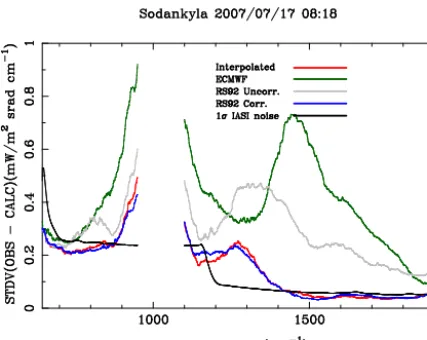
The directly observed minus calculated radiances for one particular IASI field of view (as in Figs. 3, 4, 5 and 6) con-stitute individual samples of these differences. To estimate the actual errors of these differences it is necessary to esti-mate their covariances by calculating the standard deviation within a big enough sample. To accomplish this, the values from neighbouring channels are used. This is done by obtain-ing the square root of the movobtain-ing average over a spectrum of the square of the observed minus calculated radiances. The length of the window of the moving average which is found to be useful in practice is 500 channels. In doing so, it is im-plicitly assumed that the statistical probability distribution of the errors of the 500 neighbouring channels are similar. In general this will most likely be the case, but in some circum-stances, like particular spectral absorption lines, might not be completely accurate.
The estimation of these standard deviations of the radi-ances are shown in Fig. 7 for all four cases. The ozone band is not plotted in this figure because of the big uncertainty shown in this region due to a not well characterized ozone profile. Note the very low standard deviation, below 1σ IASI instru-ment noise, for some regions of the spectrum for the “Inter-polated” and “RS92 Corr.” profiles, as already acknowledged in Calbet et al. (2011). Also recall that there is only one pa-rameter retrieved from IASI radiances when obtaining the calculated radiances, which is the surface skin temperature.
The standard deviation of the radiances difference (Fig. 7) needs to be translated from radiance space into atmospheric profile space. To do this, the OE theory Rodgers (2000) needs to be recalled by expressing the cost function,J, as J=(y−F(x))TS−1(y−F(x))
+(x−xa)TSa−1(x−xa), (1)
where y is the hyperspectral measurement, F is the radiative transfer model, Sis the measurement error covariance
Figure 7. Estimation of the standard deviation of the observed
mi-nus calculated radiance differences for each reference atmospheric profile, having removed the ozone band.
state, xa is the background state and Sa is the background
covariance matrix. This cost function is usually linearised around an atmospheric state close to the final solution, xx,
J ≈(δy−Kδx)TS−1(δy−Kδx)
+(δx−δxa)TSa−1(δx−δxa), (2)
where K is the Jacobian of F at the linearization point xx,
δx=x−xx,δxa=xa−xxandδy=y−F(xx). To find the most
likely atmospheric state or retrieval,xˆO, corresponding to a
particular IASI observation, y=yO, the derivative ofJ with respect toδx is set to zero, giving as a final retrieval solution δˆxO=(KTS−1K+S
−1 a )
−1(KTS−1
δyO+S−a1δxa), (3)
whereδˆxO= ˆxO−xxandδyO=yO−F(xx). It is known that
the error or covariance of this retrieval solution Rodgers (2000) is
Sx=(KTS−1K+S
−1 a )
−1, (4)
which is a quantity that will be needed later. A similar tech-nique can be applied to obtain the most likely state vector, xC,
corresponding to the calculated radiance, yC, obtained from applying a radiative transfer model to any of the reference atmospheric profiles,
δˆxC=(KTS−1K+S
−1 a )
−1(KTS−1
δyC+S−a1δxa), (5)
whereδxˆC= ˆxC−xx andδyC=yC−F(xx). The difference
between the two retrieved state vectors,1ˆx= ˆxO− ˆxC, gives
a quantity that measures the error in the state vector when using the calculated radiances, yC, instead of the observed ones, yO. In other words,1ˆx provides a measure of the ref-erence state quality and collocation error plus any errors we might have done in the radiative transfer model assumptions. Solving for1x givesˆ
1xˆ=(KTS−1K+Sa−1)−1(KTS−11y), (6)
Figure 8. Retrieval error (diagonal of Eq. (4) in black) and
colloca-tion and adequacy errors (1ˆx from Eq. 6) for the different reference profiles.
where1y=yO−yc. This last equation permits the conver-sion of the standard deviation radiance difference,1y, into atmospheric state space,1x. The latter will be referred to asˆ collocation and adequacy errors of the reference profiles.
Having all the necessary elements, it is now possible to define a criteria to evaluate whether a given atmospheric pro-file measurement effectively constitutes a reference propro-file for IASI. A given atmospheric profile measurement can be classified as a useful reference for IASI if the collocation and adequacy errors in the atmospheric profiles,1x from Eq. (6),ˆ is below or of the order of the retrieval error, Sxfrom Eq. (4).
The results for the four profiles are shown in Fig. 8 for tem-perature and water vapour, along with the estimated IASI retrieval error (in black) for comparison. It can be verified that the collocation and adequacy errors of the “Interpolated” and “RS92 Corr.” atmospheric profiles are of the same or-der of magnitude as the IASI retrieval error. Therefore, these two cases would qualify as reference measurements for the retrievals. The remaining two profiles, “ECMWF” and the “RS92 Uncorr.” show collocation and adequacy errors that are much larger than the retrieval errors and should not be used for validation or calibration purposes.
4 Conclusions
de-gree of coincidence between both, typically bias and standard deviation statistics. Issues like collocation uncertainties, sys-tematic errors in the humidity measurements, etc. can easily be introduced in the comparison exercise. As a consequence and as it has been shown in this paper, this methodology would, in general, grossly overestimate the uncertainties of the hyperspectral retrievals.
In this paper we propose the introduction of an additional step, after the collocation is performed, to the common val-idation methodology which consists in assessing the proper collocation and quality of the reference profiles with respect to the hyperspectral retrievals. The way to perform this as-sessment, in summary, consists of first obtaining the calcu-lated radiances by using the reference profile with as few re-trieved parameters from hyperspectral radiances as possible. These calculated radiances are then compared to the ones ob-served by the hyperspectral instrument, and a standard devi-ation as a function of wavenumber is obtained for the whole spectrum and for each particular field of view. This radiance standard deviation is then translated into an error in the atmo-spheric state space via Eq. (6), which will englobe the over-all errors in collocation and adequacy of the measurements with respect to the hyperspectral instrument. These kind of errors could be accuracy of the reference measurement pro-file, collocation uncertainties, errors in the radiative transfer modelling, non–nominal noise behaviour of the hyperspec-tral instrument, etc. If these collocation and adequacy errors are much bigger than the expected retrieval errors then these particular profiles should not be used for validation. Other-wise, the atmospheric profiles do constitute a reference mea-surement which can be used for validation and possibly cali-bration of the hyperspectral retrievals. In other words, this as-sessment checks whether the measured atmospheric profiles along with the used radiative transfer modelling and the hy-perspectral instrument measurements are consistent among each other. Another way to look at this problem is to under-stand that if the observed and calculated radiances are not consistent and compatible with each other, it will be very difficult, if not impossible, to obtain retrievals that match, within the uncertainty bounds, the measured atmospheric ref-erence profiles.
As an illustration of the method, four potential reference profiles have been tested against one particular IASI field of view measurement. Results are shown in Fig. 8. In these particular cases, the “Interpolated” (an interpolation of CFH launched 1 h before satellite overpass time and “in situ” hu-midity bias corrected RS92 sonde launched 5 min before satellite overpass time) and “RS92 Corr.” (Vömel et al., 2007 humidity bias corrected RS92 sonde launched 5 min before satellite overpass time) profiles do meet the criteria and can be used as reference atmospheric profiles. The other two, the “ECMWF” (ECMWF analysis) and the “RS92 Uncorr.” (un-corrected RS92 sonde launched 5 min before overpass time) profiles do not qualify as proper reference calibration or val-idation profiles. A feeling of what impact in selecting one
type of reference profile over another in the validation of the OE retrievals can be seen in Fig. 2. The comparison with the valid profiles that meet the selection criteria would clearly provide a better result than the comparison with the rejected ones.
An added benefit to this technique is that if there any sig-nificant issues with the comparison of profiles and retrievals they will show up in this adequacy assessment. Possible sources of errors that have been identified are large biases in the humidity measurements of RS92 radiosonde sensors Calbet et al. (2011) and possibly water vapour continuum deficiencies in the radiative transfer model Newman (2012). The technique shown in this paper is indeed a long process, and some effort needs to be invested in order to understand what are all the issues affecting the reference measurements as compared to infrared hyperspectral ob-servations until a match like the one for the “Interpolated” profiles (Fig. 3) is obtained. It is usually mandatory to understand many of the most important issues affecting all the measurements. Questions like systematic errors in the sonde humidity measurements, cloud contamination of the infrared hyperspectral observations, collocation uncertainty, calculation of the best estimate of the atmosphere, proper radiative transfer modelling, use of proper saturation water vapour function and others need to be well understood. Another downside is that the validation sample size can be reduced greatly if many of the observations are discarded because they do not meet the here described assessment criteria. Also, this method can be applied to species which are frequently measured in the atmosphere, such as tem-perature and water vapour, but it would be more difficult to apply these techniques to other components which are less often measured, such as atmospheric trace gases. On the positive side, the final selected atmospheric profiles, that have indeed passed the assessment criteria, can then be taken as truly reference profiles to validate infrared hyperspectral retrievals.
Edited by: R. Sussmann
References
Calbet, X., Schlüssel, P., Hultberg, T., Phillips, P., August, T., Vali-dation of the operational IASI level 2 processor using AIRS and ECMWF data, Adv. Space Res., 37, 2299–2305, 2006.
Calbet, X.: Determination of the best optimal estimation parame-ters for validation of infrared hyperspectral sounding retrievals, arXiv:1205.3012 [physics], 2012.
Camps-Valls, G., Munoz-Mari, J., Gomez-Chova, L., Guanter, L., Calbet, X.: Nonlinear Statistical Retrieval of Atmospheric Pro-files From MetOp-IASI and MTG-IRS Infrared Sounding Data, IEEE Trans. Geosci. Remote Sens., 50, 1759–1769, 2012. Chevallier, F.: Sampled databases of 60-level atmospheric profiles
from the ECMWF analyses, NWP SAF Doc. No. NWPSAF-EC-TR-004, 2002.
MODIS UCSB Emissivity Library: available at: http://www.icess. ucsb.edu/modis/EMIS/html/em.html (last access: 22 December 2015), 1999.
Miloshevich, L. M., Vömel, H., Whiteman, D. N., Lesht, B. M., Schmidlin, F. J., and Russo, F.: Absolute accuracy of water vapor measurements from six operational radiosonde types launched during AWEX-G and implications for AIRS validation, J. Geo-phys. Res., 111, D09S10, doi:10.1029/2005JD006083, 2006. Moncet, J. and G. Uymin and A.E. Lipton and H.E. Snell: Infrared
radiance modeling by optimal spectral sampling, J. Atmos. Sci., 65, 3917–3934, 2008.
Newman, S. M.: Report on the impact of changes in the wa-ter vapour continuum arising from the CAVIAR consortium on satellite remote sensing, Met Office RC13C Key Deliverable Re-port, February 2012.
Paukkunen, A., Antikainen, V., and Jauhiainen, H.: Accuracy and performance of the new Vaisala RS90 radiosonde in opera-tional use, paper presented at 11th Symposium on Meteorolog-ical Observations and Instrumentation, Am. Meteorol. Soc., Al-buquerque, N. M., 14–18 January 2001.
Pougatchev, N., August, T., Calbet, X., Hultberg, T., Oduleye, O., Schlüssel, P., Stiller, B., Germain, K. St., and Bingham, G.: IASI temperature and water vapor retrievals – error assessment and validation, Atmos. Chem. Phys., 9, 6453–6458, doi:10.5194/acp-9-6453-2009, 2009.
Rodgers, C. D.: Inverse methods for atmospheric sounding, Theory and practice, World Scientific, Singapore, 2000.
Smith, W. L. Sr., Harrison, F., Hinton, D., Miller, J., Bythe, M., Zhou, D., Revercomb, H., Best, F., Huang, H., Knuteson, R., To-bin, D., Velden, C. S., Bingham, G., Huppi, R., Thurgood, A., Zollinger, L., Epslin, R., and Petersen, R.: The Geosynchronous Imaging Fourier Transform Spectrometer (GIFTS) (Invited Pre-sentation), The 11th Conference on Satellite Meteorology and Oceanography (Madison, WI), 2001.
Sussmann, R., Borsdorff, T., Rettinger, M., Camy-Peyret, C., De-moulin, P., Duchatelet, P., Mahieu, E., and Servais, C.: Technical Note: Harmonized retrieval of column-integrated atmospheric water vapor from the FTIR network – first examples for long-term records and station trends, Atmos. Chem. Phys., 9, 8987– 8999, doi:10.5194/acp-9-8987-2009, 2009.
Tobin, D. C., Revercomb, H. E., Knuteson, R. O., Lesht, B. M., Strow, L. L., Hannon, S. E., Feltz, W. F., Moy, L. A., Fetzer, E. J., and Cress, T. S.: Atmospheric radiation measurement site at-mospheric state best estimates for atat-mospheric infrared sounder temperature and water vapor retrieval validation, J. Geophys. Res., 111, D09S14, doi:10.1029/2005JD006103, 2006. Vogelmann, H., Sussmann, R., Trickl, T., and Borsdorff, T.:
Intercomparison of atmospheric water vapor soundings from the differential absorption lidar (DIAL) and the solar FTIR system on Mt. Zugspitze, Atmos. Meas. Tech., 4, 835–841, doi:10.5194/amt-4-835-2011, 2011.
Vogelmann, H., Sussmann, R., Trickl, T., and Reichert, A.: Spa-tiotemporal variability of water vapor investigated using lidar and FTIR vertical soundings above the Zugspitze, Atmos. Chem. Phys., 15, 3135–3148, doi:10.5194/acp-15-3135-2015, 2015. Vömel, H., Selkirk, H., Miloshevich, L., Valverde-Canossa, J.,