www.atmos-meas-tech.net/9/741/2016/ doi:10.5194/amt-9-741-2016
© Author(s) 2016. CC Attribution 3.0 License.
Notably improved inversion of differential mobility particle
sizer data obtained under conditions of fluctuating particle
number concentrations
Bjarke Mølgaard1, Jarno Vanhatalo2, Pasi P. Aalto1, Nønne L. Prisle1, and Kaarle Hämeri1 1Department of Physics, University of Helsinki, Helsinki, Finland
2Department of Environmental Sciences, University of Helsinki, Helsinki, Finland Correspondence to: Bjarke Mølgaard ([email protected])
Received: 9 June 2015 – Published in Atmos. Meas. Tech. Discuss.: 7 October 2015 Revised: 20 January 2016 – Accepted: 2 February 2016 – Published: 29 February 2016
Abstract. The differential mobility particle sizer (DMPS) is designed for measurements of particle number size distribu-tions. It performs a number of measurements while scanning over different particle sizes. A standard assumption in the data-processing (inversion) algorithm is that the size distri-bution remains the same throughout each scan. For a DMPS deployed in an urban area this assumption is likely to be vio-lated most of the time, and the resulting size distribution data are unreliable. To improve the reliability, we developed a new algorithm using a statistical model in which the problematic assumption was replaced with more realistic smoothness as-sumptions, which were expressed through Gaussian process prior probabilities. We tested the model with data from a twin DMPS located at an urban background site in Helsinki and found that it provides size distribution data which are much more realistic. Furthermore, particle number concen-trations extracted from the DMPS data were compared with data from a condensation particle counter. At 10 min resolu-tion, the correlation for a period of 10 days was 0.984 with the new algorithm and 0.967 with the old one. Moreover, the time resolution was improved, and at 30 s resolution we ob-tained positive correlations for 89 % of the scans. Thus, the quality of the inverted data was clearly improved.
1 Introduction
There is no direct way of measuring the size distribution of fine particles. To get information on the size distribution, mo-bility particle size spectrometers (Wiedensohler et al., 2012) select in turns particles of various electrical mobilities, and for each electrical mobility the number of particles in some volume is counted. To obtain the size distributions, the de-pendence of electrical mobilities on particle sizes is utilised. However, the electrical mobility depends also on the particle charge, so various combinations of particle size and charge give the same electrical mobility, and the inference of the ac-tual particle size distribution is not trivial. The algorithms which have been developed for this purpose are generally known as inversion algorithms. The task can be split into two parts: determination of the transfer function, which gives the detection probabilities of particles in the sampled air, and the actual inversion. In this study we focused on the latter part. Further we restrict ourselves to considering differential mobility particle sizers (DMPSs) which differ from scanning mobility particle sizers (SMPSs) by changing the selected electrical mobility in discrete steps.
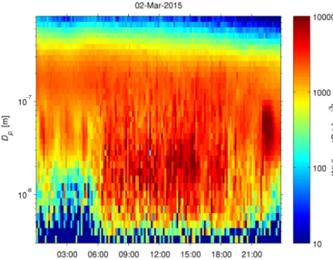
dis-Figure 1. Size distributions from 2 March 2015 according to the
old inversion algorithm, which assumes stationary particle size dis-tributions during each scan.
tribution changes slowly most of the time, this assumption is reasonable most of the time. However, when a DMPS is de-ployed in a city with numerous nearby sources and a turbu-lent wind flow, this assumption is often far from the truth, and many of the derived particle size distributions are unreliable. Let us illustrate this with an example using inverted data from the twin DMPS (comprises two DMPSs) at the SMEAR III (Station for Measuring Ecosystem–Atmosphere Relations) station in Helsinki (Järvi et al., 2009) on 2 March 2015. The particle size distribution fluctuated substantially during day-time (Fig. 1), but at night-day-time there were periods without fluctuations. For these night-time periods, the particle size distribution was a rather smooth function of size, but in day-time unrealistically narrow peaks are present in the inverted data. In particular, the scan from 11:00 to 11:10 UTC+2 h is problematic, because of the strong, narrow peaks at 13 and 30 nm (Fig. 2). Single-charged particles of these two sizes are measured almost simultaneously in the two DMPSs, so the peaks at these sizes are most likely caused by a brief con-centration peak. At 26 nm dN/dlog10Dp appears to be low
(Fig. 2; see also the light-blue spot close to the middle of Fig. 1), although the raw data indicate that the concentration was already elevated when the DMPS measured particles at this size. However, a fraction of the particles in the 30 nm bin will be detected in the measurement centred at 26 nm, and, assuming a stationary particle size distribution, the 30 nm particles were very abundant also during this measurement. Thus, assuming a stationary particle number size distribu-tion, most of the particles detected in this measurement be-longed to the 30 nm bin. Additionally, double-charged 39 nm particles contributed somewhat to the particle count. As a re-sult, a small value was assigned to dN/dlog10Dpat 26 nm.
10−9 10−8 10−7 10−6 0
0.5 1 1.5 2 2.5
3x 10
4
d
N
/dlog
10
(D
p
) [cm
−3
]
D p [m]
10:50−11:00 UTC+2h 11:00−11:10 UTC+2h 11:10−11:20 UTC+2h
Figure 2. Three particle number size distributions from 2 March
2015 according to the old inversion algorithm, which assumes sta-tionary particle size distributions during each scan.
A few studies have addressed this issue of possible size distribution changes happening during a scan. Voutilainen and Kaipio (2001) presented an algorithm based on the Kalman filter. They let the particle size distribution change in discrete steps at each measurement based on the obser-vation and a random walker. Subsequently, a smoother and a non-negativity constraint were applied. The algorithm was applied to synthetic data, and it reproduced a slowly varying size distribution well. Voutilainen and Kaipio (2002, 2005) parametrised the size distribution and replaced the random walker by estimations of the time evolution based on an aerosol model which took coagulation and condensation into account. The underlying assumption is that the DMPS con-tinuously samples from the same aerosol, which changes in time due to these processes. Also this assumption is generally invalid in a city. Although the algorithm by Voutilainen and Kaipio (2005) was also shown to adjust to abrupt changes in the aerosol within a couple of minutes, it was not designed for use in urban locations.
2 Methods
2.1 Quantification of particle size distributions
Particle size distributions are usually described by the dN/dlog10Dp, although it is not a distribution function
in a mathematical sense. N is the product of the total particle number concentration and the cumulative distribu-tion funcdistribu-tion of the particle diameters (Hinds, 1999). Thus, dN/dlog10Dp is the product of the concentration and the
probability density function on the logarithmic scale. 2.2 DMPS
The DMPS comprises a neutraliser (bi-polar charger), a dif-ferential mobility analyser (DMA), and a condensation par-ticle counter (CPC). In the neutraliser, ionising radiation en-sures that the particles in the sampled air reach the equilib-rium charge distribution. This charge distribution is known and depends on the particle size. In the DMA, the voltage and airflow are adjusted to select particles with a certain elec-trical mobilityZ= qCc
3π ηDp, whereq is the charge;Dpis the
mobility (Stokes’) diameter;Ccis the Cunningham slip cor-rection factor, which depends onDp; andηis the dynamic
viscosity of the air. SoZdepends on two particle properties: Dpandq=ze, wherezis an integer andeis the elementary
charge. The particles selected by the DMA flow to the CPC which counts them. Usually, the flows are kept constant and the DMPS scans over a few tens of discrete DMA voltages in order to select particles of different electrical mobilities. At each of these voltages, a measurement is performed with the CPC.
2.3 Transfer function
The transfer functionT (Dp, U )is defined as the probability
that a particle of diameterDp will be detected in the CPC
when the DMA voltage isU. This probability is the product of the following three probabilities:
– PDMA, the probability that the particle is selected by the DMA (Stolzenburg, 1988; Mamakos et al., 2007); – PPen, the probability that the particle penetrates all
sam-pling lines without being deposited (Wiedensohler et al., 2012);
– PCPC, the detection probability for particles reaching the CPC.
The DMA is designed to select particles with electric mo-bilities in a narrow band. The electric mobility depends on Dpand the numberzof charges. The probability of a certain
numberzof charges depends on the particle size, i.e. onDp.
Thus,PDMA can be described as a function of Dp and the
DMA voltageU. Diffusion is the main reason for deposition of particles in the sampling lines, and the particle diffusiv-ity depends on the particle size, so PPen is also a function
ofDp.PCPC is close to unity (1) for most particles, but for
the smallest particles it is lower. During a measurementithe DMA voltage is kept at a constant valueUi. We will define
Ti(Dp)=T (Dp, Ui). Ti has a few clear peaks and is zero
for the rest of the interval. The largest peak is for the diam-eter which gives the selected electrical mobilityZwhen the number of chargeszequals 1 or−1. The sign depends on the polarity of the DMA voltage. A second peak is observed for the diameterDp, which gives the same electrical mobility for
a particle with double charge. This peak is smaller than the first one, because particles are less likely to carry two charges than one charge. Triple-charged particles cause a third peak, which is smaller than the second peak, and subsequent peaks are even smaller.
2.4 Inversion algorithm based on a GP model
A GP, or Gaussian random field, is a stochastic process that can be used to define probability distributions over functions, and it is a generalisation of the multivariate normal (Gaus-sian) distribution (O’Hagan, 1978; Rasmussen and Williams, 2006). It is defined by a mean and a covariance function, which determine the properties, such as the smoothness and variability of the process. GPs are widely used for interpo-lation and to model coloured (spatially correlated) noise in spatial statistics (Gelfand et al., 2010), and they have ob-tained increasing interest also in, e.g., statistics and machine learning due their good interpolation and smoothing proper-ties as well as convenient marginalisation and conditioning properties (see Sect. 2.5.2) (Rasmussen and Williams, 2006; Vanhatalo et al., 2010).
Let us define a latent function f (t, u)=log(dN/du), wheret is time andu=log10Dp. We use the Bayesian
for-malism and express our prior belief about its smoothness through a GP prior. Thus, the posterior, which is proportional to the product of the prior and the likelihood, is a probability distribution off.
2.4.1 Likelihood function
Each measurementiprovides a countyi of particles, so the
Poisson distribution Poi(yi|λi)=exp(−λi) λyii
yi! is suitable for
each factor of the likelihood p(y|f )=Y
i
exp(−λi)
λyi
i
yi!
. (1)
The rate parameterλi is obtained by integrating the product
of dN/dlog10Dpand the transfer functionTi. In terms off
andudefined above,
λi=Q ∞
Z
−∞ ti,end
Z
ti,begin
exp(f (t, u))Ti(10u)dtdu, (2)
does not fluctuate much during each measurement (which has much shorter duration than a scan), the following approxima-tion holds:
λi≈Vi ∞
Z
−∞
exp(f (ti, u))Ti(10u)du, (3)
whereVi is the volume of sampled air andti is the middle
of the time interval betweenti,beginandti,end. BecauseTihas
a few clear peaks and is zero for the rest of the interval, the integral can be well approximated by a sum. LetTi,j equal
the integral ofTi over the peak centred at sizeui,j, and let
fi,j =f (ti, ui,j). Then
λi≈Vi
X
j
exp(fi,j)Ti,j. (4)
The number of peaks to consider in this sum depends on the size of the selected particles. When the DMA selects parti-cles with high electrical mobility (meaning very small par-ticles), Ti,2Ti,1, because these particles have very small probability of carrying two charges. On the other hand, for particles with diameters of a few hundred nanometres, mul-tiple charges are common, and we considered particles with up to six charges (following the custom of the old inversion algorithm).
2.4.2 Prior
The particle number size distribution is assumed to be a smooth function of the particle size, and it is assumed to vary smoothly over time. These properties are modelled by giving a GP prior for the latent function
f (t, u)∼GP(µ(t, u), k(u, u0)k(t, t0)), (5) where µ(t, u) is the mean function and k(u, u0)k(t, t0) is the covariance function such that k(u, u0)=
Cov(f (t, u), f (t, u0))andk(t, t0)=Cov(f (t, u), f (t0, u)). We assume that the mean function is constant,µ(t, u)=
µ, so that it represents the average off and give it a Gaus-sian prior µ∼N (0, σµ2). This implies that the prior can be written asf (t, u)∼GP(0, σµ2+k(u, u0)k(t, t0)). The covari-ance function along the particle size follows the Matérn co-variance function with 5/2 degrees of freedom (Rasmussen and Williams, 2006):
k(u, u0)=σ2 1− √
5|u−u0| lu
+5|u−u
0|2
3lu2 !
e− √
5|u−u0|/lu, (6)
whereσ2governs the magnitude of process variation andlu
governs the autocorrelation length of the GP along the par-ticle size dimension. The covariance function along the time domain is exponential:
k(t, t0)=e−|t−t0|/lt, (7)
whereltis the autocorrelation length of the GP along the time
dimension. The Matérn and exponential covariance functions lead to a stationary process in particle size and time di-mension. The exponential covariance function corresponds to a continuous-time autoregressive model of order one and is mean-square continuous, but not mean-square differen-tiable (see, e.g., Rasmussen and Williams, 2006). The Matérn covariance function with 5/2 degrees of freedom is twice mean-square differentiable, for which reason our construc-tion leads to a process that is smoother along the particle size than time dimension.
The prior variance of mean σµ2=10, leading to rela-tively flat (vague) prior distribution. The covariance func-tion parameters, θ= {σ, lt, lu}, are given weakly
informa-tive half Studentt priors (Gelman, 2006) so thatσ, lt, lu∼
Studentt+(ν=4, s2), which is the Student t distribution
scaled and restricted to positive values. The scale parameters s2are 3, 0.01 days, and 0.25.
2.5 Implementation
2.5.1 Data from the SMEAR III station in Helsinki We used data from the urban background station SMEAR III (Järvi et al., 2009). In some wind directions, traffic emis-sions affect the sampled aerosol substantially (see the map in Fig. 3). The particle size distributions were measured with a twin DMPS (two DMPSs running in parallel). Each DMPS used a Hauke-type DMA and a butanol CPC from TSI. In each scan, DMPS-1 performed 15 measurements in the size range 3–40 nm using a short DMA (10.9 cm) and CPC model 3025, and DMPS-2 performed 30 measurements in the range 15–820 nm using a long DMA (28 cm) and CPC model 3010. Following the custom used with the old inversion algorithm, we discarded the first three DMPS-2 measurements due to high uncertainty in the transfer function and thereby reduced the size range to 23–820 nm. The measurements varied in duration from 5.6 to 70.2 s in DMPS-1 and from 4.8 to 9.2 s in DMPS-2. The longest measurements were for the smallest particle sizes. Between consecutive measurements, there was a lag time of about 12 s, which was needed for the voltage change and for flushing the sampling tube between the DMA and the CPC. The time stamps of individual measurements were not recorded until recently, so we had to reconstruct them. The uncertainty of the reconstructed time stamps are estimated to be 2 s at the end of a scan and less than that at the beginning of a scan.
We got the transfer function from the old inversion algo-rithm used at University of Helsinki. For each measurement i, we integrated the transfer functionTi for each peak
sep-arately to get the valuesTi,j in Eq. (4). However, as
SMEAR III
University
Campus
Vegetated
area
100 m Major road
Minor road
Figure 3. Neighbourhood of the SMEAR III station.
as 10−4for DMPS-1, and 10−3for DMPS-2. Furthermore, we used the common assumption that the concentration of particles larger than 1 µm is negligible (Wiedensohler et al., 2012). With these choices, we got about 130 training inputs
xi,j =(ti, ui,j)for each scan as illustrated in Fig. 4.
In our pre-processing of the data we also had to recon-struct the particle counts in all measurements by multiply-ing the saved concentrations, sample flows, and durations of measurements. We rounded the results of this multiplication to get integer counts. This reconstruction may be affected by rounding errors, which, however, are of secondary impor-tance.
We processed data from 26 February to 7 March 2015 in batches of eight scans. After fitting the model to the data, for the post-processing we defined a grid with 5 s time resolution and 59 points covering diameters from 3 to 1000 nm. For this grid, we calculated expected val-ues and variance of f (E[f] and Var[f]). In our poste-rior approximation (Sect. 2.5.2) dN/dlog10Dp=dN/du=
exp(f )is log-normally distributed, so E[dN/dlog10Dp] =
exp(E[f] +0.5Var[f]). By numerical integration over the particle size we obtained expected values for the particle number concentration. To estimate the uncertainties of these concentrations, for each time point we first drew a sample of 200 size distributions from the posterior and calculated par-ticle number concentrations based on these, and then we cal-culated 80 % posterior intervals for the particle number con-centration. Consecutive batches were overlapping each other, having two scans in common. The post-processed results from the individual batches were merged. For the 10 min in the middle of the overlap, the merged results were calculated as weighted averages with the weights gradually changing from one batch to the next one.
We did all calculations on a normal desktop computer. For each batch the model fitting took about 2 min, and another 2 min were spent on the post-processing. The sampling of
Time [hh:mm] UTC+2h
11:00 11:02 11:04 11:06 11:08 11:10
D p
[m]
10-9 10-8 10-7 10-6
DMPS-1 DMPS-2
Figure 4. Training inputs for the scan on 2 March between 11:00
and 11:10 UTC+2 h. For clarity we put Dp instead ofu on the
vertical axis (yaxis).
size distributions was the most time-consuming part of the post-processing.
Independent measurements of particle number concentra-tions were obtained with a CPC (TSI 3787 water CPC), which detected particles larger than 5 nm. The time resolu-tion fluctuated a bit and was approximately 5 s. These data were only used for evaluating the results obtained with our inversion algorithm.
2.5.2 Inference
Given the model description and data, we approximate the posterior distribution (Gelman et al., 2013) of f (t, u) as follows. Let y= {y1, . . ., yn}T denote the n counts of
par-ticles at times of measurement t= {t1, . . ., tn}T; let f= {fT1,·, . . .,fTn,·}Tdenote all the latent variables needed to de-fine the likelihood; and letu= {uT1,·, . . .,uTn,·}denote the
cor-responding log particle sizes. Here, fi,·= {fi,j}j:Ti,j>αTi,1
andui,·= {ui,j}j:Ti,j>αTi,1 denote all the latent variables and
sizes corresponding to timeti for whichTi,j is greater than
the thresholdαTi,1. Due to the marginalisation property of
GP, the prior for the latent variables isf|t,u,θ∼N (0,K), whereKl,m=Cov(fl, fm). The conditional posterior of the
latent variables, given the hyperparameters, is then
p(f|y,t,u,θ)∝N (f|0,K)5ni=1p(yi|f), (8)
wherep(yi|f)=Poi(yi|ViPjexp(fi,j)Ti,j). Motivated by
approximation:
p(f|y,t,u,θ)≈q(f|y,t,u,θ)=N (f| ˆf,6), (9)
where6−1= −∇∇log(p(f|y,t,u,θ))|
f= ˆf is the Hessian of the negative log-conditional posterior at the mode. The mode fˆ is found by a modification of a Newton al-gorithm. The aim is to maximise 9(f)=logp(y|f)+
logp(f|t,u,θ), for which the basic Newton iteration is
fnew=fold−(∇∇9)−1∇9 (10)
=fold+(K−1+W)−1(∇logp(y|fold)−K−1fold), (11)
where W= −∇∇logp(y|fold). We initialised the optimi-sation withf =0. Direct calculation of the inverse of6=
K−1+W might be numerically unstable, so we used the form
6−1=L I+LTWL−1LT, (12)
where LLT=K is the Cholesky decomposition of the co-variance matrix. Moreover, the likelihood is not a log-concave function off, for which reason6may not be posi-tive definite at early iteration steps far from modefˆ. In fact, in our experience this is the usual case. For this reason we check whether I+LTWL is positive definite and, if not, make the Newton iteration
fnew=fold+(K−1+We)
−1(∇logp(y|fold)−K−1fold), (13)
where Wel,m=max(Wl,m,0) if l=m and Wel,m=0
otherwise. Here, the implementation uses the nu-merically more stable form (K−1+W)e −1=K−
KWe1/2 I+We1/2KWe1/2 −1
e
W1/2K obtained using the Sherman–Morrison–Woodbury lemma (Rasmussen and Williams, 2006).
The hyperparameters, θ, are set to their ap-proximate maximum a posterior (MAP) estimate
ˆ
θ=arg maxθq(y|t,u,θ)p(θ), where q(y|t,u,θ) is the approximate marginal likelihood of the hyperparameters,
q(y|t,u,θ)≈p(y|t,u,θ)=
Z
p(y|f)p(f|t,u,θ)df. (14)
The integral on the right-hand side is not analytically tractable, for which reason we use the Laplace approximation a second time. We form a second-order Taylor expansion of 9(f)aroundfˆ so that9(f)≈9(fˆ)−1
2(f− ˆf)
T6−1(f−
ˆ
f). Now the marginal likelihood can be approximated with a
Gaussian integral overf multiplied by a constant q(y|t,u,θ)=exp(9(fˆ))
Z
exp
−1
2(f− ˆf)
T6−1(f− ˆf)
df. (15) The logarithm of the marginal likelihood is then (see Ap-pendix A of Vanhatalo et al., 2010)
logq(y|t,u,θ)
= −1
2
ˆ
fTK−1fˆ +logp(y| ˆf)−1
2log(|K||6|) (16)
= −1
2
ˆ
fTK−1fˆ+logp(y| ˆf)−1
2log |I+L
TWL|
. (17) The MAP estimate of the hyperparameters can now be searched for by maximising logq(y|t,u,θ)+logp(θ).
It is possible to analytically solve the gradients of logq(y|t,u,θ) with respect to θ (see Rasmussen and Williams, 2006), which allows the use of gradient-based op-timisation. We used the scaled conjugate gradient method available in the Matlab toolbox GPstuff (Vanhatalo et al., 2013) and optimised the hyperparameters on a log scale.
After findingθˆand constructing the Gaussian approxima-tion for the condiapproxima-tional posteriorp(f|y,t,u,θˆ), we can use these approximations to calculate the (approximate) poste-rior predictive distribution off (t, u) at any {t, u}. Due to the marginalisation properties of a GP, the posterior predic-tive mean and variance off (t, u)can be calculated exactly if we know the posterior mean and variance off (Vanhat-alo, 2010). Because we cannot solve these quantities exactly, we approximate the posterior predictive mean as (Vanhatalo, 2010)
E[f (t, u)|y,t,u,θˆ] =kTK−1E[f|y,θˆ] ≈kTK−1fˆ
=kT∇logp(y| ˆf), (18)
wherekis a vector with elementskl=Cov(f (t, u), fl)and
the last equality comes from the fact that
∇logp(y|f)+logp(f|t,u,θˆ)| f= ˆf
= ∇logp(y| ˆf)−K−1fˆ =0. (19)
Similarly, the posterior predictive variance is approximated as
Var[f (t, u)|y,t,u,θˆ]
=Var[f (t, u)] −kTK−1−K−1Cov[f|y,t,u,θˆ]K−1k (20)
≈Var[f (t, u)] −kTK−1−K−1K−1+WK−1k (21)
=Var[f (t, u)] −kTK+W−1−1k (22)
10−9 10−8 10−7 10−6 0
500 1000 1500 2000 2500
d
N
/dlog
10
(D
p
) [cm
−3
]
D p [m]
Old inversion 03:40−03:50 UTC+2h 03:40 UTC+2h
03:45 UTC+2h 03:50 UTC+2h
Figure 5. The size distribution obtained with the old inversion
al-gorithm and expected size distributions (new inversion) for a period with little fluctuation on 26 February.
lemma and Eq. (12). Given the approximate posterior mean and variance for f (t, u) at any {t, u}, it is natural to ap-proximate the posterior distributionp(f (t, u)|y,t,u,θˆ)with a Gaussian distribution with the above mean and variance. The above-described Laplace approximation has been shown to produce accurate estimates for the marginal likelihood p(y|t,u,θ)and conditional posteriorp(f|y,t,u,θ)in sev-eral models with similar structure (Tierney and Kadane, 1986; Rue et al., 2009; Vanhatalo et al., 2010, 2013).
3 Results and discussion
We will evaluate the results from our algorithm both by look-ing at some illustrative examples and by comparlook-ing result-ing particle number concentrations for the whole period with CPC data.
As a first test of the algorithm, let us consider periods with-out fluctuations, meaning periods for which the old algorithm performed well. As expected, for these periods our results agree well with the results from the old algorithm. The only clear difference is that we obtain smoother size distributions with our new algorithm as in the example in Fig. 5. Espe-cially, in the region below 20 nm the old algorithm gave an uneven result due to low count statistics (ranging from 0 to 7 particles in each measurement). The smoother size distribu-tions seem more plausible and were, indeed, obtained using a proper description of the count statistics in the likelihood function as described in Sect. 2.4.1 (the smoothness was also affected by the prior).
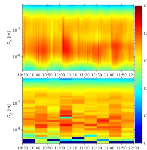
In our next example (2 March 10:30–12:00 UTC+2 h) the evolution of the size distribution was as shown in Fig. 6. Clearly, the total particle number concentration fluctuated a lot, and some changes in the size are also seen. At any given time, dN/dlog10Dpchanges smoothly as a function of
size. The variances in Fig. 7 reflect the distance in time and
Figure 6. Upper panel: expected size distributions on 2 March
be-tween 10:30 and 12:00 UTC+2 h. Lower panel: size distributions for the same period obtained with the old inversion algorithm. The ticks on the time axis (xaxis) denote the beginnings of scans.
Figure 7. Posterior variance off on 2 March between 10:30 and 12:00 UTC+2 h. The ticks on the time axis (xaxis) denote the be-ginnings of scans.
particle size to the nearest measurements: the further these measurements are, the greater the variance is. In Fig. 4 we showed the training inputs for one scan, and in Fig. 7 low-variance areas appear around the training inputs of nine sub-sequent scans.
10:300 10:40 10:50 11:00 11:10 11:20 11:30 11:40 11:50 12:00 0.5
1 1.5 2 2.5
3x 10 4
Time [hh:mm]
Particle number concentration [cm
−3
]
DMPS
DMPS old inversion CPC
Figure 8. Particle number concentrations on 2 March between 10:30 and 12:00 UTC+2 h.
concentration. The reason for this difference is that the CPC measurements are not corrected for particle losses in the sam-pling lines. The peaks generally occur at the same time, al-though a few of the peaks in the CPC data are not reflected in concentrations obtained from the DMPS. For instance, the peak at 10:49 UTC+2 h is only seen in the CPC data. At this time, DMPS-1 measured 3 nm particles, and DMPS-2 mea-sured particles with diameters of more than 500 nm. No clear signs of an elevated concentration are seen in these measure-ments, and thus no inversion algorithm will be able to repro-duce this peak. In general, with the set-up of our twin DMPS, peaks occurring during the last 3–5 min of a scan are often not observed. On the other hand, when both DMPSs measure in the range from 10 to 50 nm, fluctuations in the concentra-tion are most likely observed and our algorithm is able to ex-tract these fluctuating concentrations well. For instance, the peak occurring around 11:03 UTC+2 h was well observed by the twin DMPS. With the old inversion algorithm, this peak was clearly a problem (as described in the Introduc-tion), but with our new algorithm we obtained good agree-ment with the CPC data. Some expected size distributions are plotted together with the result of the old inversion algo-rithm in Fig. 9. Obviously, our new algoalgo-rithm provided size distributions which are much more realistic, but we do not know how close these estimates are to the actual size distri-butions, because we have no size distribution data from other instruments. In general, the size information during peaks is limited because of the low number of DMPS measurements available.
Even less size information is available for the brief concentration peak occurring between 11:31:25 and 11:32:00 UTC+2 h. According to the CPC measurements, the top of the peak occurred at 11:31:50 UTC+2 h, which was during the waiting time in both DMPSs, so the peak is not as high according to the DMPS measurements. The few DMPS measurements which were affected by this
concentra-10−9 10−8 10−7 10−6 0
0.5 1 1.5 2 2.5
3x 10
4
d
N
/dlog
10
(D
p
) [cm
−3
]
Dp [m] Old inversion 11:00 − 11:10 11:00:35
11:02:35 11:04:35 11:06:35
Figure 9. Expected size distribution before, during, and after the
peak on 2 March at 11:03 UTC+2 h, and the result of the old inver-sion algorithm for the scan between 11:00 and 11:10 UTC+2 h.
tion peak were all for particles in the size range 19 to 23 nm, and these suggested higher dN/dlog10Dp at 19 nm than at
23 nm, although this difference could be due to temporal fluctuation. Our algorithm gives the size distribution seen in Fig. 10 at 11:31:45 UTC+2 h; as expected, dN/dlog10Dp
shows a decrease between 19 and 23 nm. The sampled size distributions give examples of what the size distribution may have looked like, and they have maxima between 13 and 20 nm. This seems reasonable given the available size information and the general low values of dN/dlog10Dp
10−9 10−8 10−7 10−6 0
0.5 1 1.5 2 2.5x 10
4
d
N
/dlog
10
(D
p
) [cm
−3
]
Dp [m]
E[dN/dlog10Dp] Draw 1 Draw 2 Draw 3 Draw 4 Draw 5
Figure 10. Expected size distribution with 95 % posterior intervals
and five size distributions sampled from the posterior for 2 March at 11:31:45 UTC+2 h.
fluctuations are simultaneous with the fluctuations at smaller sizes (see Fig. 6). This is caused by the smoothing in size. Fast fluctuations are not observed when the DMPS measures in the accumulation mode, so we do not expect them to occur in the accumulation mode at other times either. The accumulation mode particles have a long lifetime in the atmosphere and may originate from distant sources, while the particles smaller than 25 nm most likely originate from nearby traffic emissions (Hussein et al., 2014). However, we used a stationary covariance function with two length scales lu and lt. Because of differences in lifetime and
origin, it would make more sense to use a non-stationary covariance function with a long timescale at diameters of a few hundreds of nanometres and a short timescale for smaller particles. In practice, however, implementing such a covariance function is not straightforward. With the current covariance function, lt will be a compromise between the
actual timescales at different sizes. Thus, we expect too much smoothing in the time dimension at small diameters and, as noted above, too little at larger diameters.
To evaluate the performance for the processed 10-day pe-riod, we compared mean particle number concentrations ob-tained from the DMPS and the CPC data at 10 min and 30 s resolution. At 10 min resolution the correlation between the means from the two instruments was 0.984. For comparison, when processing the DMPS data with the old inversion al-gorithm, the obtained correlation (0.967) was twice as far from 1 (i.e. from perfect correlation). At the higher time res-olution we calculated correlations for each scan separately, and Fig. 11 shows a histogram of these correlations. Clearly, for most scans there is a good correlation, and our algo-rithm extracts information of the time evolution, which was lost with the old algorithm. However, for 11 % of the scans, the correlation is negative, reflecting a disagreement between
−1 −0.5 0 0.5 1
0 50 100 150 200 250
Correlation
Number of scans
Figure 11. Histogram of correlations between 30 s mean particle
number concentrations obtained from the DMPS and the CPC. The correlations are calculated for each scan separately.
10:300 10:35 10:40 10:45 10:50 10:55 11:00 200
400 600 800 1000 1200 1400 1600 1800
Time [hh:mm]
DMPS
DMPS old inversion CPC
Figure 12. Particle number concentrations on 7 March between
10:30 and 11:00 UTC+2 h.
time evolutions obtained from the DMPS with our algorithm and from the CPC. We have investigated all eight cases for which the correlation is smaller than−0.75. In two cases the concentration was almost constant according to both instru-ments, and it seems that small fluctuations caused the nega-tive correlation by chance. In the remaining cases, concentra-tion changes not observed by the DMPS seem to be at least part of the reason.
Let us illustrate this with an example (Fig. 12). For the time interval 10:40–10:50 UTC+2 h, the correlation was
10:45 UTC+2 h, so the slightly elevated concentration was not observed. This elevation ended at 10:50 UTC, and the counts during the following scan suggest a lower concentra-tion, so our algorithm suggests a smooth decrease of the con-centration in the time interval 10:45–10:50 UTC+2 h. Also during the first 5 min of the scan (10:40–10:45 UTC+2 h) we observe decreasing concentration according to the DMPS and increasing concentration according to the CPC. How-ever, it seems that our model fits that data well also dur-ing this period, meandur-ing that the counts y agree well with the rate parameters λ (data not shown). If we specifically consider the first 2 min of each of the scans in Fig. 12, the CPC showed on average slightly lower concentration dur-ing 10:40–10:42 UTC+2 h than during the other 2 min pe-riods. However, comparing these three periods, one finds that the DMPS counts were clearly highest during 10:40– 10:42 UTC+2 h. This gives some indication that the rela-tively high concentration in the beginning of this scan is sup-ported by the DMPS data. The negative correlation during this scan seems to originate from the measurements rather than from any problem in our inversion algorithm. Our in-vestigation of other scans with negative correlations did not suggest problems with the inversion either. So despite these occasional negative correlations, it seems that our model ex-tracts the information of the concentration time evolution well from the available DMPS measurements.
The results above are based on a few simplifying as-sumptions. We assumed that the particle concentration only changes a little during each measurement. This is not nec-essarily always the case, but the approximation in Eq. (3) is correct at least at some point during the measurement. For DMPS-2 most of the measurements are short (∼5 s), and any error arising from this approximation can be consid-ered as a minor error in the timing. For DMPS-1, each mea-surement at the smallest sizes last around 1 min, but strong fluctuations are rare at these sizes. In principle, we could have split the time intervals into smaller pieces and summed up their contribution, but the minor improvement would not have justified the extra computational cost. We ignored parti-cles larger than 1 µm, but with the chosen data this seems to be a minor issue. We also ignored the uncertainties of sam-ple and sheath flows, so our uncertainties are somewhat un-derestimated. The sample flows affect the likelihood directly through Eq. (2), and all flows affect the transfer function. Other small inaccuracies in the transfer function may arise from inaccurate determination of diffusional losses and dif-fering charging probabilities of non-spherical particles, such as agglomerates from diesel exhaust (Maricq, 2008).
In summary, our algorithm extracts well the time evolu-tion of the particle number concentraevolu-tion from the available DMPS data, and in the absence of fluctuations the obtained size distributions fit well with results from the old algorithm. During fluctuations, only little information about the parti-cle sizes is available, and the uncertainties of the size distri-butions are considerable. Due to a lack of independent size
distribution data, a quantitative evaluation of the size distri-butions obtained for periods with fluctuation was impossible, but there is no doubt that these size distributions are much closer to the truth than the ones obtained with the old algo-rithm.
In principle, this method should work for the SMPS as well, but we expect the implementation to be more diffi-cult. The continuous scan needs to be divided into a num-ber of counting intervals. If the counting intervals are long, the peaks of the transfer function will be much wider. On the other hand, if the counting intervals are short, the number of training inputs in our model will be high, and our algorithm will be much slower.
4 Conclusions
We have developed a new algorithm (provided in the Sup-plement) based on a Gaussian process model for process-ing DMPS data, and we tested it with data from a twin DMPS in an urban background location. Our algorithm de-rives dN/dlog10Dp as a function of Dp and t based on
DMPS measurements and smoothness assumptions. Because these assumptions are more realistic than the assumption of a stationary aerosol, the derived size distributions are also much more realistic. We compared particle number con-centrations with independent CPC measurements and found a good agreement.
The higher accuracy of the particle number size distribu-tions can benefit studies of aerosols in urban locadistribu-tions and other places with fluctuating size distributions. The higher time resolution is useful, for instance, when attempting to pinpoint sources, given that other data, such as wind obser-vations, exist at a good time resolution. Particle number size distributions at a high time resolution can be obtained with other instruments as well, but this algorithm offers an im-provement both for existing and future DMPS data without any need to purchase new hardware.
The Supplement related to this article is available online at doi:10.5194/amt-9-741-2016-supplement.
Acknowledgements. J. Vanhatalo and N. L. Prisle were funded by
the Academy of Finland (grants 266349 and 257411, respectively).
Edited by: S. Malinowski
References
Gelman, A.: Prior distributions for variance parameters in hierar-chical models, Bayesian Analysis, 1, 515–533, doi:10.1214/06-BA117A, 2006.
Gelman, A., Carlin, J. B., Stern, H. S., Dunson, D. B., Vehtari, A., and Rubin, D. B.: Bayesian Data Analysis, 3rd edn., Chapman and Hall/CRC, Boca Raton, FL, USA, 675 pp., 2013.
Hinds, W. C.: Aerosol Technology: Properties, Behavior, and Mea-surement of Airborne Particles, John Wiley and Sons, Inc., Hobo-ken, NJ, USA, 504 pp., 1999.
Hussein, T., Mølgaard, B., Hannuniemi, H., Martikainen, J., Järvi, L., Wegner, T., Ripamonti, G., Weber, S., Vesala, T., and Hämeri, K.: Fingerprints of the urban particle number size distri-bution in Helsinki, Finland: local versus regional characteristics, Boreal Environ. Res., 19, 1–20, 2014.
Järvi, L., Hannuniemi, H., Hussein, T., Junninen, H., Aalto, P. P., Hillamo, R., Mäkelä, T., Keronen, P., Siivola, E., Vesala, T., and Kulmala, M.: The urban measurement station SMEAR III: Con-tinuous monitoring of air pollution and surface-atmosphere in-teractions in Helsinki, Finland, Boreal Environ. Res., 14 (Sup-plement A), 86–109, 2009.
Mamakos, A., Ntziachristos, L., and Samaras, Z.: Diffusion broadening of DMA transfer functions. Numerical valida-tion of Stolzenburg model, J. Aerosol Sci., 38, 747–763, doi:10.1016/j.jaerosci.2007.05.004, 2007.
Maricq, M. M.: Bipolar diffusion charging of soot aggregates, Aerosol Sci. Tech., 42, 247–254, doi:10.1080/02786820801958775, 2008.
O’Hagan, A.: Curve fitting and optimal design for prediction, J. Roy. Stat. Soc. B Met., 40, 1–42, 1978.
Rasmussen, C. E. and Williams, C. K. I.: Gaussian Processes for Machine Learning, The MIT Press, Cambridge, MA, USA, avail-able at: www.gaussianprocess.org/gpml (last access: 1 October 2015), 2006.
Rue, H., Martino, S., and Chopin, N.: Approximate Bayesian in-ference for latent Gaussian models by using integrated nested Laplace approximations, J. Roy. Stat. Soc. B, 71, 1–35, doi:10.1111/j.1467-9868.2008.00700.x, 2009.
Stolzenburg, M. R.: An ultrafine aerosol size distribution measur-ing system, PhD thesis, Department of Mechanical Engineermeasur-ing, University of Minnesota, USA, 1988.
Tierney, L. and Kadane, J. B.: Accurate approximations for pos-terior moments and marginal densities, J. Am. Stat. Assoc., 81, 82–86, 1986.
Vanhatalo, J.: Speeding Up the Inference in Gaussian Process Mod-els, PhD thesis, School of Science and Technology, Aalto Uni-versity, Finland, 126 pp., 2010.
Vanhatalo, J., Pietiläinen, V., and Vehtari, A.: Approximate infer-ence for disease mapping with sparse Gaussian processes, Stat. Med., 29, 1580–1607, doi:10.1002/sim.3895, 2010.
Vanhatalo, J., Riihimäki, J. P., Hartikainen, J., Jylänki, P., Tolva-nen, V., and Vehtari, A.: GPstuff: Bayesian Modeling with Gaus-sian Processes, J. Mach. Learn. Res., 14, 1175–1179, 2013. Voutilainen, A. and Kaipio, J. P.: Estimation of non-stationary
aerosol size distributions using the state-space approach, J. Aerosol Sci., 32, 631–648, doi:10.1016/S0021-8502(00)00110-5, 2001.
Voutilainen, A. and Kaipio, J. P.: Estimation of time-varying aerosol size distributions – exploitation of modal aerosol dynamical models, J. Aerosol Sci., 33, 1181–1200, doi:10.1016/S0021-8502(02)00062-9, 2002.
Voutilainen, A. and Kaipio, R.: Sequential Monte Carlo estimation of aerosol size distributions, Comput. Stat. Data An., 48, 887– 908, doi:10.1016/j.csda.2004.03.011, 2005.