www.clim-past.net/6/565/2010/ doi:10.5194/cp-6-565-2010
© Author(s) 2010. CC Attribution 3.0 License.
Climate
of the Past
Statistical issues about solar–climate relations
P. Yiou1,*, E. Bard2, P. Dandin3, B. Legras4, P. Naveau1, H. W. Rust1, L. Terray5, and M. Vrac1
1Laboratoire des Sciences du Climat et de l’Environnement, UMR CEA-CNRS-UVSQ 8212, IPSL, Gif-sur-Yvette, France 2Centre Europ´een de Recherche et d’Enseignement des G´eosciences de l’Environnement, UMR 6635,
Aix-en-Provence, France
3M´et´eo-France, Division de la Climatologie, Toulouse, France
4Laboratoire de M´et´eorologie Dynamique, UMR 8539, IPSL, Ecole Normale Sup´erieure, Paris, France 5Centre Europ´een de Recherche et Formation Avanc´ees en Calcul Scientifique, Toulouse, France
Received: 23 March 2010 – Published in Clim. Past Discuss.: 7 April 2010 Revised: 29 July 2010 – Accepted: 4 August 2010 – Published: 8 September 2010
Abstract. The relationship between solar activity and tem-perature variation is a frequently discussed issue in climatol-ogy. This relationships is usually hypothesized on the basis of statistical analyses of temperature time series and time se-ries related to solar activity. Recent studies (Le Mou¨el et al., 2008, 2009; Courtillot et al., 2010) focus on the variabilities of temperature and solar activity records to identify their re-lationships. We discuss the meaning of such analyses and propose a general framework to test the statistical signifi-cance for these variability-based analyses. This approach is illustrated using European temperature data sets and ge-omagnetic field variations. We show that tests for significant correlation between observed temperature variability and ge-omagnetic field variability is hindered by a low number of degrees of freedom introduced by excessively smoothing the variability-based statistics.
1 Introduction
The detection and attribution of climate change has been extensively investigated with various statistical methods (Hegerl et al., 2007). The role of solar activity on climate has been examined by many authors with climate models (Haigh, 1994; Shindell et al., 2001; Hansen et al., 2005; Meehl et al., 2009) and by comparing statistically solar and global or re-gional climate records (e.g. Lean and Rind, 2008, 2009; Ben-estad and Schmidt, 2009). Although weak in terms of energy balance, it seems to have played a significant role in vari-ous episode during the last millennium (Jansen et al., 2007).
Correspondence to: P. Yiou ([email protected])
There is an on-going debate on the exact role of solar ac-tivity on 20th century temperature variations. Siscoe (1978) pointed out flaws of the many papers debating on the subject, more than 30 years ago. More recently, Lockwood (2008) provided a critical assessment of the potential mechanisms linking solar variations to climate change, and showed that solar variations are not sufficient to explain the 20th cen-tury warming from elementary laws of physics and thermo-dynamics.
Three papers have recently reported statistical analyses of temperature and solar activity records (Le Mou¨el et al., 2008, 2009; Courtillot et al., 2010). Those papers introduce and discuss an unconventional method for time series analysis (at least in climate sciences). Those authors claim that this method (called “Mean Squared Deviation”) gives informa-tion on the time evoluinforma-tion of the autocorrelainforma-tion of a random process with slow heteroscedasticity. Our paper illustrates some statistical properties of such a transform, and provides tests of its significance from simple random processes. Those authors use European daily temperature records, and a record of geomagnetic intensity as a proxy for solar activity. Al-though this choice is debatable, we decided to be as close as possible as the framework of (Le Mou¨el et al., 2008, 2009).
1900 1920 1940 1960 1980 2000
6
8
10
12
14
Years
T mean
Paris De Bilt Europe mean
Fig. 1. Variations of the annual averages of daily mean temperature in Paris, De Bilt and a European mean, between 1900 and 2009. The data are taken from the ECA&D database (Klein-Tank et al., 2002).
hypotheses are formulated and proper statistical tests are per-formed. When mathematical transforms (such as the mean squared deviation) are involved, such tests should explore the sensitivity of the results to the parameters of the transforms.
Section 2 describes the data sets used in the paper. The methodology is detailed in Sect. 3. Three types of results are provided in Sect. 4.
2 Data
We used the daily mean temperature from the ECA&D database in Europe (Klein-Tank et al., 2002). In particular, we randomly focused on the Paris-Montsouris (France) and De Bilt (Netherlands) stations between 1900 and 2009.
We also used a set of European temperatures starting be-fore 1920 and ending after 2000, and yielding less than 10% of missing or doubtful data. We computed the spatial average for each day of this data set, although its spatial distribution tends to give a lot of weight to Central Europe. The annual means of the three data sets are shown in Fig. 1. They all exhibit a warming over the 20th century. The exceptional warming between 2004 and 2009 in the European mean is due to the fact that a large proportion of “cold” stations (from central to eastern Europe) have systematic missing values af-ter 2004. Thus, when the arithmetic mean of the ensemble is computed after 2004, it tends to be pulled toward higher tem-peratures. This feature should not be interpreted as an excep-tional warming, but is an effect of missing data in ECA&D
1920 1940 1960 1980 2000
45000
45500
46000
Z component
(a)
1920 1940 1960 1980 2000
−150
−50
0
50
100
Year
Z anomaly
(b)
Fig. 2. (a) Daily variations of theZcomponent of the geomagnetic field measure at Eskdalemuir between 1911 and 2008. The red line represents the smoothed data with a spline function with 20 degrees of freedom. (b) Anomaly of theZcomponent with respect to the spline smoothing function.
stations after 2004. We point out that the problem of miss-ing data also appears before 1940. Such a problem could be circumvented by removing a seasonal cycle from tempera-ture data. Hence all time series are centered (i.e. with zero mean), as well as their average. Thus, there is no artificial drift of the mean due to missing observations. We computed a mean seasonal cycle from the daily temperature data for the 1960–1990 period, and we removed it from the raw time se-ries to obtain daily anomalies of temperature. We hence used daily temperature anomalies in computations of this paper. For brevity, the term “temperature” now refers to “anoma-lies of temperature with respect to a seasonal cycle”, unless otherwise specified.
Homogeneity problems have been detected on daily time steps, and to our knowledge they have not been corrected in the ECA&D database (O. Mestre, personal communica-tion, 2009). The lack of homogeneity (due to changes in instruments, orientation or simply reporting errors) can gen-erate artificial non-climatic discontinuities. In this paper, we do not question or evaluate the quality of the temperature data, although most stations are indicated as “suspect” on the ECA&D database. This evaluation is done in a further study (Legras et al., 2010).
geomagnetic field are measured in many stations around the earth. The intensity of the geomagnetic field is dominated by dynamo processes of the interior of the earth, varying on secular time scales. The fast variations, on time scales of minutes to years, are mainly influenced by solar activity and galactic cosmic rays, as discovered by Sabine, Wolf, Gau-tier and Lamont in the 19th century. It is then reasonable to assume that the fast variations recorded by stations over the Earth mostly reflect the fluctuations of solar activity (see Bartels, 1932, for a review). The intensity of the geomag-netic field is measured in three directions. It appears that the fast variability of the horizontal and vertical components are very similar (Le Mou¨el et al., 2009). Thus we focus on the vertical component variations (Z) of the geomagnetic field.
In this study, we followed the choice of Le Mou¨el et al. (2009) and used the geomagnetic data from Eskdalemuir (UK) as a proxy for solar activity. The data was obtained from the World Data Center for Geomagnetism (www.wdc. bgs.ac.uk/catalog/master.html). We computed daily averages from the hourly data, from 1911 to 2008. The time series shows a steady increase since 1938 (Fig. 2). This trend re-flects secular changes in the geomagnetic field. We thus con-sider the small variations around this trend.
Mean daily temperature and geomagnetic times series have no mutual correlation (see Table 1, first column). Hence, the investigation of a potential relationship between the two variables motivates a focus on other statistical diag-nostics. The next section gives an example of such analysis.
3 Method
Auto-regressive processes of order 1 (AR(1)) are often used in climate studies to define a null hypothesis to describe vari-ations of temperature time series (Allen and Smith, 1994; Ghil et al., 2002; Maraun et al., 2004). By definition, an AR(1) processR(t )is:
R(t+1)=aR(t )+b(t ), (1)
where 0≤a <1 andb(t )is a centered white noise with un-known but finite varianceσb2. The parametera gives infor-mation on the memory of the process from one time step to the next. We use this simple random process as a pedagogical benchmark for the study of variability properties of time se-ries, because they can be explicitly derived for various kinds of quadratic transforms. This process is commonly denoted “red noise” because its power spectrum decreases with fre-quency (Priestley, 1981).
Such a model can be refined to include slow time varia-tions ofa andσ. Such variations alter the probability distri-bution ofR(t )and an exaustive list of the properties of such processes lies beyond the scope of this paper (e.g. Embrechts et al., 2000).
For a given centered time seriesX(t )(of observations, for example), one wants to find an AR(1) process that fits “best”
the statistical characteristics of X(t ), like its variance and auto-covariance. The classical maximum likelihood estimate (MLE)aˆforagives (Priestley, 1981):
ˆ
a=CX(1)
CX(0)
, (2)
whereCX(0)is the sample variance ofX andCX(τ )is its
sample auto-covariance at lagτ:
CX(τ )=
1 N−τ
N−τ
X
t=1
X(t+τ )X(t ).
For the AR(1) processR of Eq. (1), the auto-covariance is (Priestley, 1981):
CR(τ )=
σb2a|τ|
1−a2. (3)
An alternative approach, suggested by Le Mou¨el et al. (2009), is to define the mean squared daily variation: ζ2(t )
for a given time window2:
ζ2(t )=
1 2
t+2/2
X
τ=t−2/2
(X(τ+1)−X(τ ))2. (4)
For an AR(1) process (R(t )in Eq. (1)), the expected value of ζ2R(t )converges to:
E[ζ2R] = 2σ
2 b
1+a,
for all2. This can be verified by expanding Eq. (4) and using Eq. (3).
The mean interannual squared variationQ2(t )is defined
as:
Q2(t )=
1 2
t+2/2
X
τ=t−2/2
(X(τ+365)−X(τ ))2. (5)
For an AR(1) processR(t ), the expected value ofQR(t ) con-verges to:
E[QR2] = 2σ
2 b
1−a2,
for all2. We note that bothE[ζ2R(t )]andE[QR2(t )]depend onaandσbfor an AR(1) process, but not on2.
The “lifetime” function is defined by Le Mou¨el et al. (2009) as the normalization ofQ2(t )byζ2(t ):
L2(t )=Q2(t )/ζ2(t ). (6)
This denomination is not connected with the lifetime notion in statistical survival theory (e.g. Lawless, 2003). For an AR(1) process, it follows that the expected value of LR2(t ) is:
E[LR2(t )] = 1
0 5 10 15 20
0
5
10
15
20
25
True lambda
Estimated lambda
●●
●●
●●
●● ●
●●
●●
●●
● ●● ●
● ●
●●
● ● ●
● ● ●
●●
● ●● ●
●●
● ●
● ● ●
●● ●
● ●
● ●
●● ●●
●● ●● ●
●● ●●
●● ● ●● ●
● ● ● ●
● ● ● ●
● ● ●●
● ●●
● ●
●● ● ●●
● ●● ●●
● ●●
0 0.75 0.9 0.925 0.95 a
●
●
L(t) estimate MLE estimate
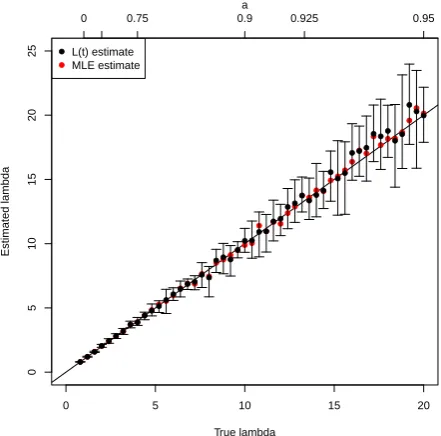
Fig. 3. Bias estimates ofλfrom an MLE computationλˆ(red circles)
and mean “lifetime” computationλ¯(black circles). The bars around theλ¯ estimates indicate the 5th and 95th quantiles ofL
2(t )
varia-tions of AR(1) realizavaria-tions. See text for formulas. The first diagonal is indicated for reference. The upper axis indicates variations ofa
(as in Eq. (1)).
The interesting point of this quotient is that it no longer de-pends onσbfor an AR(1) process. Thus for a given2, we
obtain an estimatorλ¯ forλ:
¯
λ=mean(L2(t )),
where mean(.)is the sample mean overt. Thus, in princi-ple, the L2(t )transform can be used to estimate a for an
AR(1) process (a¯=1−1/λ¯). However, the properties (bias, variance) are not a priori known but can be assessed by sim-ulation (see next section). As a consequence of this con-vergence, it is hoped that ifa varies slowly in time (over a scale larger than2) in Eq. (1), then it should be possible to estimate the variation rate from Eq. (6). This motivates the L2(t )transform.
The MLE estimate ofain Eq. (2) also provides an estimate ofλ:
ˆ
λ= 1
1− ˆa.
The second goal of the paper is to obtain the signifi-cance of correlations between the transformationsL2(t) and
Q2(t )of two time seriesXandY.
In general, the non nullity of a correlationrXY between
two time seriesXandY can be tested with a Student t-test (von Storch and Zwiers, 2001):
t= |rXY|
n−2
1−rXY2
1/2
, (8)
wherenis the number of dregrees of freedom inX andY. From the value oft, one can derive a p-value that is the risk of wrongly rejecting the null hypothesisrXY=0 (von Storch
and Zwiers, 2001). The value ofnis a priori lower than the number of data points. When transforms such asQ2(t )or
L2(t )are applied, the upper bound forncan be estimated
byn≈N/2, whereN is the number of data points. If the time series cover one century on daily time steps and2=
11×365, then the number of degrees of freedomnforQ2(t )
andL2(t )isn≈10.
We remind that when a significant correlation is found be-tween two time series there is no proof (or even a suggestion) of causality between the variables because correlation is a symmetric operator. A fortiori, finding a correlation between theL2,Q2orζ2quadratic transforms of two time seriesX
andY does not provide any causality relation betweenXand Y.
4 Results 4.1 Bias
The first step of this study is to verify that theL2(t )
trans-form is indeed a practical estimator ofλ, i.e. with satisfactory properties of convergence and bias. We designed an ensem-ble of numerical experiments with AR(1) processes, by sam-pling the(0,20)interval ofλvalues with increments of 0.4. From those samples ofλ, we takea(=1−1/λ), and simulate AR(1) processes, with a unit varianceσb2forb(t )(in Eq. (1)). The experiments are carried onN=30000 increments. For each realization, we computedL2(t )with2=11×365 and
its averageλ¯. We also determined the variance and
autoco-variance, to estimateaˆin a direct way from Eq. (2). We then plotted the values ofλˆ for both estimates, as functions of the
“real”λ from which the processes were constructed. The choice of2=11×365 is somewhat arbitrary. Its heuristic justification is that it covers a sunspot cycle of≈11 years. The exact length of2should not alter theL2estimates if an
interpretation in term of memory needs to be done.
The results (Fig. 3) show that the MLE estimateλˆ
gener-ally performs well. The “lifetime” estimateλ¯ does not yield an apparent bias. The confidence intervals forλ¯ seem to in-crease witha, indicating a higher variability ofL2(t )whena
(orλ) increases. This is explained by the singularity ata=1. This exercise can be performed on the Paris or De Bilt temperature data. We obtain respectively aˆ≈0.8 anda¯≈
1900 1920 1940 1960 1980 2000
18
20
22
24
26
Q(t)
●
(a) De Bilt
1900 1920 1940 1960 1980 2000
4.0
4.5
5.0
5.5
6.0
L(t)
● ● ●
Θ Θ=7yr Θ Θ=11yr
Θ Θ=22yr
(b) De Bilt
1900 1920 1940 1960 1980 2000
20
22
24
26
28
Q(t)
●
(c) Paris
1900 1920 1940 1960 1980 2000
4.5
5.0
5.5
L(t)
● ● ●
Θ Θ=7yr Θ Θ=11yr
Θ Θ=22yr
(d) Paris
Q(t)
1900 1920 1940 1960 1980 2000
3.5
4.0
4.5
5.0
5.5
6.0
6.5
●
(e) Europe
L(t)
1900 1920 1940 1960 1980 2000
10
12
14
16
18
20
22
● ● ●
●
(f) Europe
Θ Θ=7yr Θ Θ=11yr
Θ Θ=22yr
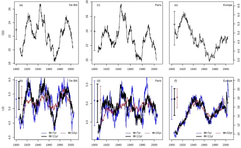
Fig. 4. (a) Variations of dailyQ2(t )for De Bilt temperature between 1900 and 2008, with2=11 years. (b) Same convention as (a) with L2(t ). The colored continous lines show the variations ofL2(t )when the parameter2is varied from 7 years to 22 years. (c) Same as (a)
for the mean daily Paris temperature. (d) same as (b) for the mean daily Paris temperature. (e) Same as (a) for the mean daily European temperature. (f) same as (b) for the mean daily European temperature. The vertical confidence intervals indicate the median, 5th and 95th quantiles for the variations ofQ2(t )(orL2(t )) of an AR(1) process with the same variance and auto-covariance.
ofλ¯ of the European mean temperature in term of process
memory is a priori not possible.
4.2 Variability ofQ2(t)andL2(t)for temperature
The second step of the study is to investigate the range of variations ofQ2(t )(the mean squared daily variations) and
L2(t )for a random process (AR(1)). From Eq. (2), we
deter-minedaˆandσˆ for the De Bilt and Paris temperature anoma-lies. This allows us to simulate AR(1) processes having the same variance and autocovariance (and length) as those perature series. For each random realization and the tem-perature data, we computedQ2(t ),ζ2(t )andL2(t ). We
determined the 5th, 50th and 95th quantiles of Q2(t ) and
L2(t ).
The variations ofQ2(t )for De Bilt and Paris temperature
anomalies and the 90% bounds for red noise are shown in Fig. 4a, c. Overall, the large deviations ofQ2(t )are
signif-icant, with respect to an AR(1) process. The variations of L2(t )for temperature anomalies (Fig. 4b, d) show generally
similar shapes as those ofQ2(t )for De Bilt and Paris and
they are also significant with respect to an AR(1) process.
We note that when the window 2increases from 11 to 22 years, some of the maxima ofL2(t )lose their significance
with respect to an AR(1) process (Fig. 4b, d). Curiously, the variations ofQ2(t )andL2(t )are different for the mean
European temperature. This can be explained by the fact that the statistical properties of the mean of time series are not the same as individual series, in particular in term of persistence. We note that the L2(t ) transform for raw temperature
(i.e. without removing the seasonal cycle) has the same gen-eral behavior and order of magnitude as for the temperature anomalies. This feature motivates the use ofL2(t )to
inves-tigate the variability of time series with periodic components that are potentially complex.
We checked the dependence of the analysis on2in the L2(t )estimate. Indeed, the interpretation of a single
out-standing “event” in L2(t ) should be robust to the choice
of the window 2 in Eq. (6). We hence computed L2(t )
with2=7,11 and 22 years (Fig. 4b) for the De Bilt and Paris daily temperature. This illustrates that an alteration in the window size changes important details of the transform L2(t ). This provides an additional (albeit more heuristic)
ζζ
(t)
200
600
1000
Q(t)
1920 1940 1960 1980 2000
40
60
80
100
ζζ(t) Q((t)) (a)
1920 1940 1960 1980 2000
2
5
10
20
L(t)
(b)
Fig. 5. (a)Q2(t ) of the geomagnetic data (blue line). Mean
squared daily deviation (ζ2(t )) ofZ(black line). The confidence
intervals are computed for the mean squared daily deviationζ2(t )
between 1940 and 2008. (b)L2(t )of the geomagnetic data with 2=11 years. The confidence intervals are determined for this pa-rameter between 1940 and 2008 (vertical line).
If De Bilt or Paris temperature series are considered, the ma-jor peaks or troughs ofQ2(t )andL2(t )found for2=11
years seem unstable to this parameter, and it is not reasonable to load them with a physical interpretation.
We have also applied the analysis to the ensemble mean of temperature from the ECA&D database. The auto-correlation functionCX(1)of the ensemble daily mean is
larger than for each station. The time variation for the en-semble mean are coherent with the De Bilt or Paris data, but with a higher baseline (Fig. 4e, f). The conclusions of the significance of the variations ofL2(t )remain for ensemble
averages of temperature.
4.3 Significance of correlations
Should one persist in usingL2(t )as an estimator of
variabil-ity for a time series, the next question that arises is the sig-nificance of correlations between two transformed data sets. TheL2(t )transform intrinsically reduces the number of
de-grees of freedom of a time series: ifN is the number of data samples,Ndofthe number of degrees of freedom of the data,
then the number of degrees of freedom ofL2(t )is
approx-imated by min(Ndof,N/2). In other words, the number of
degrees of freedom ofL2(t )is bounded by the number of
independent windows in the sum in Eq. (6). Further filters, like moving averages or splines, also contribute to the reduc-tion of the number of degrees of freedom in a time series.
The goal here is to compare the time variations of the Q2(t ) and L2(t ) functions of two time series X and Y
through their correlation. The idea of this approach is to compare the variability ofX andY, although both time se-ries might be uncorrelated. In any case, we repeat that the correlation betweenL2(t )transforms does not allow for an
inference of a mutual relation between the original time se-ries, unless a specific model of covariation is provided.
L1L2 Q1Q2 zeta1zeta2
0.0
0.2
0.4
0.6
|r|
0.4
0.25
0.14
0.07
0.02
p value
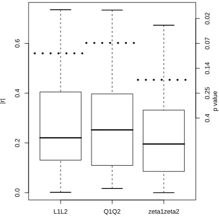
Fig. 6. Distribution of absolute values of correlation|r|between
L2(t ), Q2(t )and ζ2(t ) transforms of two random AR(1)
pro-cesses with the respective variance and autocovariance of ECA&D European temperatures and geomagnetic field from Eskdalemuir. The box and whisker plots indicate the 25, 50 and 75th quantiles
q(boxes). The upper whisker corresponds to: min(max(|r|),q50+
1.5×(q75−q25)). The right hand vertical axis shows the p values
forr=0.3 to 0.7, with increments of 0.1, corresponding to a null hypothesis of no correlation andn=10 degrees of freedom. The horizontal thick dotted lines indicate the 90th quantile of|r|values.
It should be noted that correlatingζ2 variations of one
variable withL2 variations of another variable is very
dif-ficult to justify. Indeed, ζ2 measures mean fluctuations of
one day to the next, andL2 measures fluctuations of days
separated by one year. Nevertheless, in order to have an ex-tensive view of the correlations among transforms of tem-perature and geomagnetic data, we compute the correlations between theL(t ) transforms of temperature data sets, and ζ (t ),Q(t )andL(t )transforms for geomagnetic data.
From the behavior of the geomagnetic data (Fig. 5a), it is reasonable to subtract the low frequency part of the time series, which is connected to slow internal dynamo pro-cesses, and not relevant to solar activity. We hence smoothed the data with a spline function with 20 degrees of freedom (Green and Silverman, 1994), and retained the anomalies with respect to this spline function. We verified that those anomalies do not have a trend. TheL2(t )andQ2(t )
The first step is to estimate the probability of spurious correlation ofL2(t ),Q2(t )andζ2(t )for two independent
AR(1) processes X and Y. For the sake of the exercise, we computed the variance and autocovariance of mean daily temperature over Europe and the geomagnetic field intensity anomalies. We then generated 100 independent realizations of each AR(1) process over 30000 time steps (approximat-ing the number of days dur(approximat-ing the 20th century), and com-putedL2(t ),ζ2(t )andQ2(t )for each realization. We took
2=11 years for those experiments.
The correlation distributions show that it is relatively fre-quent (with probability p >0.1) that the correlations be-tween Q2(t ) of two independent processes exceed 0.5 in
absolute value (Fig. 6). The p-values of correlations for n≈10 degrees of freedom are below 0.07 only whenr > 0.6, see Fig. 6 (right axis). This implies that L2(t ) or
Q2(t )transforms of two independent AR(1) processes with
the same covariance features (variance and lag-1 auto-covariance) as temperature and geomagnetic field are likely to yield large absolute values of correlation. Conversely, this means that large absolute values of correlation forL2(t )or
Q2(t )transforms do not necessarily imply statistical
signifi-cance. This emphasizes the importance of correlation testing, especially when the number of degrees of freedom is low.
In a second step, we computedζ2(t ),Q2(t )andL2(t )
for the geomagnetic daily anomaly data anomalies, with the same parameters as Le Mou¨el et al. (2009).
From the geomagnetic anomalies, we determined the AR(1) process with the same variance and covariance, to es-timate confidence intervals. Theζ2(t )andQ2(t )variations
are overall significant with respect to an AR(1). The vari-ations ofL2(t )are generally not significant after 1940
be-cause their amplitude is smaller than for an AR(1) process. The L2(t )and Q2(t ) variations present a major decrease
near 1940, andL2(t )yields relatively weak variations
af-ter this date. The reasons for this change are undocumented, but could come from changes of instrument, or measurement frequency.
The (linear) correlations between theL2(t )of daily mean
temperature (resp. Paris, De Bilt and European average) andL2(t )of Z are generally weak and not significant, as
sumarized in Table 1. The correlation even changes signs when European mean temperature is considered. The cor-relations between L2(t )of temperatures and Q2(t ) of Z
are also weak and not significant. The correlations between L2(t ) of temperatures and ζ2(t ) of Z is higher, and can
reachr=0.61. But the p-value of the correlation isp >0.06, which still make it unsignificant by usual standards, because of the low number of degrees of freedom.
Overall, this shows that no conclusion about a covariation diagnostic can be derived from the comparison of theL2(t ),
Q2(t )orζ2(t )transforms of temperature and geomagnetic
activity. We also point out that higher correlation values (al-though not significant) are obtained with a special choice of transforms, which have no a priori justification. Thus,
chos-Table 1. Correlations betweenζ2,Q2andL2transforms of daily
temperature series and theZcomponent of the geomagnetic field, between 1940 and 2009 (2=11×365). p-values forn=10 de-grees of freedom are indicated in parentheses when the correlation coefficient exceeds 0.4. Correlations under 0.4 are not considered significant.
Variables Z ζZ QZ LZ
TParis 0.07
LParis 0.52 (0.12) 0.14 0.08
TDeBilt 0.06
LDeBilt 0.53 (0.11) 0.33 0.26
TEurope 0.04
LEurope 0.61 (0.06) 0.30 −0.43 (0.21)
ing different kinds of data transforms (i.e. L2(t )vs. ζ2(t ))
to compare two data sets, in order to maximize a correlation can potentially lead to “data snooping”.
4.4 Identification of causality inL2(t)
Although none of the transforms outlined above provide tools to assess any causal link between two variables, one may assume that such a relationship exists, and determine the amplitude of the link. For example, consider two generalized AR(1) variablesXandYsuch that the memory parameteraY is controled by a functionFX(t ), i.e. aY(t )=FX(t ). The question we want to address is whetherLY(t )is correlated to the functionFX(t ).
In general, the answer to such a question is negative be-cause Eq. (7) is not true whena varies continuously (even slowly) with time. We illustrate this point by creating a gen-eralized AR(1) process:
R(t+1)=a(t )R(t )+b(t ), (9)
where 0≤a(t ) <1 slowly with time andb(t )is a white noise with zero mean. In this example, we setX to be the mean squared daily variation of theZcomponent of the geomag-netic data after 1940 andY is a mean daily temperature in Paris modeled by the generalized AR(1) process of Eq. (9).
We find that the correlation betweenLY2(t ) and ζ2(Z)(t ) is generally positive (in 90% of cases), although the median correlation isr=0.53 and is hence not significant because of the low number of degrees of freedom (n=7). This synthetic example shows that when the causality between memory pa-rametersa(t )is assumed, then theL(t )transforms is barely sufficient to retrieve the original forcing function. This poor score, even in an idealized case, is due to the fact that the variance ofb(t ) plays a role inL(t )whena(t )varies with time in Eq. (9), although it does not appear in Eq. (7). This further illustrates that an interpretation ofL(t )for a general-ized AR(1) process with varyinga(t )cannot be obtained in a satisfactory manner. In general,L(t )does not allow for an estimate of the time variations of the parameters of a general-ized AR(1) process, unless those variations follow stepwise constant functions (as outlined by Le Mou¨el et al. (2009)). If the underlying process is more complicated than an AR(1) (for example if the variance ofb(t ) also varies with time), then the interpretation ofL(t )in terms of process memory is impossible.
5 Conclusions
We analyzed the potential ofL2(t ),ζ2(t )andQ2(t )
trans-forms of time series to characterize the variability of a time series. Using elementary statistical techniques of hypothe-sis testing, based on Monte Carlo simulations, we have pro-vided a framework to check the statistical significance of such transforms, and hence help with their physical interpre-tation.
Following Le Mou¨el et al. (2009), we applied those pro-cedures to temperature and geomagnetic activity time series. We found that theζ2(t ),Q2(t )andL2(t )variations of those
variables are generally significant with respect to an AR(1) process. Moreover, a rigorous test between both variables shows that no significant correlation exists between them. Of course, we do not exclude that such transforms would not give significant results with other data sets.
This study can be extended to other transforms and sta-tistical diagnostics. We emphasize the importance of testing statistical estimates with respect to reasonably chosen null hypotheses in order to avoid data snooping. In the case of L2(t ), the most reasonable and simple null hypothesis is an
AR(1) process, for whichL2(t )has a direct interpretation.
But temperature variations generally cannot be modelled by an elementary AR(1) process (Huong Hoang et al., 2009; Yiou et al., 2009). If time variations ina andσb are
intro-duced in Eq. (1), their contribution to theζ2(t )andQ2(t )
transforms cannot be separated as simply as for an AR(1). This strongly limits the use and interpretation of those trans-forms to diagnose the variability of a time series.
Finally, we point out that all the results presented in this paper are based on second order statistics of time series. The L2 diagnostic omits variations of first order, i.e. variations
of the mean. From a quick inspection of Fig. 1, it is clear that the mean temperature evolves with time on multi-annual time scales. None of the presented analyses allow to explain such a temperature variation with a geomagnetic series. The in-crease of temperature (or temperature anomalies) after 1940 is still unexplained by the variations of the geomagnetic field anomalies.
Supplementary material related to this article is available online at:
http://www.clim-past.net/6/565/2010/ cp-6-565-2010-supplement.zip.
Acknowledgements. We thank P. Besse, D. Dacunha-Castelle,
M. Ghil, V. Masson-Delmotte, O. Mestre and A. Ribes for valuable discussions and input. All computations were done in the R language (www.r-project.org). The R code to produce the figures is available on the Clim. Past server as supplementary material to this paper.
Edited by: H. Goosse
The publication of this article is financed by CNRS-INSU.
References
Allen, M. and Smith, L. A.: Investigating the origins and signifi-cance of low-frequency modes of climate variability, Geophys. Res. Lett., 21, 883–886, 1994.
Bard, E., Raisbeck, G., Yiou, F., and Jouzel, J.: Solar modulation of cosmogenic nuclide production over the last millennium: com-parison between C-14 and Be-10 records, Earth Planet. Sc. Lett., 150, 453–462, 1997.
Bartels, J.: Terrestrial-magnetic activity and its relations to solar phenomena, J. Geophys. Res. (Terr. Magn. Atmos. Electr.), 37, 1–52, doi:10.1029/TE037i001p00001, 1932.
Beer, J., Siegenthaler, U., Bonani, G., Finkel, R., Oeschger, H., Suter, M., and Wolfli, W.: Information On Past Solar-Activity And Geomagnetism From Be-10 In The Camp Century Ice Core, Nature, 331, 675–679, 1988.
Benestad, R. E. and Schmidt, G. A.: Solar trends and global warm-ing, J. Geophys. Res.-Atmos., 114, doi:10.1029/2008JD011639, 2009.
Cliver, E., Boriakoff, V., and Feynman, J.: Solar variability and climate change: Geomagnetic aa index and global surface tem-perature, Geophys. Res. Lett., 25, 1035–1038, 1998.
Embrechts, P., Kluppelberg, C., and Mikosch, T.: Modelling Ex-tremal Events, Springer-Verlag, 2000.
Ghil, M., Allen, M. R., Dettinger, M. D., Ide, K., Kondrashov, D., Mann, M. E., Robertson, A. W., Tian, Y., Varadi, F., and Yiou, P.: Advanced Spectral Methods for Climatic Time Series, Rev. Geophys., 40, 1–41, 2002.
Green, P. J. and Silverman, B. W.: Nonparametric regression and generalized linear models: a roughness penalty approach, Mono-graphs on statistics and applied probability; 58, Chapman & Hall, London; New York, 1st edn., 1994.
Haigh, J.: The role of stratospheric ozone in modulating the solar radiative forcing of climate, Nature, 370, 544–546, 1994. Hansen, J., Sato, M., Ruedy, R., Nazarenko, L., Lacis, A., Schmidt,
G., Russell, G., Aleinov, I., Bauer, M., Bauer, S., Bell, N., Cairns, B., Canuto, V., Chandler, M., Cheng, Y., Del Genio, A., Falu-vegi, G., Fleming, E., Friend, A., Hall, T., Jackman, C., Kelley, M., Kiang, N., Koch, D., Lean, J., Lerner, J., Lo, K., Menon, S., Miller, R., Minnis, P., Novakov, T., Oinas, V., Perlwitz, J., Perlwitz, J., Rind, D., Romanou, A., Shindell, D., Stone, P., Sun, S., Tausnev, N., Thresher, D., Wielicki, B., Wong, T., Yao, M., and Zhang, S.: Efficacy of climate forcings, J. Geophys. Res.-Atmos., 110, doi:10.1029/2005JD005776, 2005.
Hegerl, G., Zwiers, F. W., Braconnot, P., Gillett, N., Luo, Y., Orsini, J. M., Nicholls, N., Penner, J., and Stott, P. A.: Understand-ing and AttributUnderstand-ing Climate Change, in: Climate Change 2007: The Physical Science Basis. Contribution of Working Group I to the Fourth Assessment Report of the Intergovernmental Panel on Climate Change, edited by: Solomon, S., Qin, D., Manning, M., Chen, Z., Marquis, M., Averyt, K., Tignor, M., and Miller, H., Cambridge University Press, Cambridge, UK and New York, NY, USA, 2007.
Hoyt, D. and Schatten, K.: Group Sunspot Numbers: A new solar activity reconstruction, Sol. Phys., 179, 189–219, 1998. Huong Hoang, T. T., Parey, S., and Dacunha-Castelle, D.:
Mul-tidimensional trends: The example of temperature, Eur. Phys. J.-Spec. Top., 174, 113–124, doi:10.1140/epjst/e2009-01094-6, 2009.
Jansen, E., Overpeck, J., Briffa, K., Duplessy, J.-C., Joos, F., Masson-Delmotte, V., Olago, D Otto-Bliesner, B., Peltier, W., Rahmstorf, S., Ramesh, R., Raynaud, D., Rind, D., Solomina, O., Villalba, R., and Zhang, D.: Palaeoclimate, in: Climate Change 2007: the physical science basis: contribution of Working Group I to the Fourth Assessment Report of the Intergovernmental Panel on Climate Change, edited by Solomon, S., Qin, D.and Manning, M., Chen, Z., Marquis, M., Averyt, K., Manning, M., and Miller, H., chap. 6, Cambridge University Press, Cambridge, New York, 2007.
Klein-Tank, A., Wijngaard, J., Konnen, G., Bohm, R., Demaree, G., Gocheva, A., Mileta, M., Pashiardis, S., Hejkrlik, L., Kern-Hansen, C., Heino, R., Bessemoulin, P., Muller-Westermeier, G., Tzanakou, M., Szalai, S., Palsdottir, T., Fitzgerald, D., Rubin, S., Capaldo, M., Maugeri, M., Leitass, A., Bukantis, A., Aber-feld, R., Van Engelen, A., Forland, E., Mietus, M., Coelho, F., Mares, C., Razuvaev, V., Nieplova, E., Cegnar, T., Lopez, J., Dahlstrom, B., Moberg, A., Kirchhofer, W., Ceylan, A., Pachal-iuk, O., Alexander, L., and Petrovic, P.: Daily dataset of 20th-century surface air temperature and precipitation series for the European Climate Assessment, Int. J. Climatol., 22, 1441–1453, 2002.
Lawless, J. F.: Statistical models and methods for lifetime data, Wi-ley series in probability and statistics, WiWi-ley-Interscience, Hobo-ken, N.J., 2nd edn., 2003.
Le Mou¨el, J.-L., Courtillot, V., Blanter, E., and Shnirman, M.: Ev-idence for a solar signature in 20th-century temperature data from the USA and Europe, C. R. Geosci., 340, 421–430, doi:10.1016/j.crte.2008.06.001, 2008.
Le Mou¨el, J.-L., Blanter, E., Shnirman, M., and Courtillot, V.: Evi-dence for solar forcing in variability of temperatures and pres-sures in Europe, J. Atmos. Sol.-Terr. Phys., 71, 1309–1321, doi:10.1016/j.jastp.2009.05.006, 2009.
Lean, J. L. and Rind, D. H.: How natural and anthropogenic in-fluences alter global and regional surface temperatures: 1889 to 2006, Geophys. Res. Lett., 35, doi:10.1029/2008GL034864, 2008.
Lean, J. L. and Rind, D. H.: How will Earth’s surface tem-perature change in future decades?, Geophys. Res. Lett., 36, doi:10.1029/2009GL038932, 2009.
Legras, B., Mestre, O., Bard, E., and Yiou, P.: On mislead-ing solar-climate relationship, Clim. Past Discuss., 6, 767–800, doi:10.5194/cpd-6-767-2010, 2010.
Lockwood, M.: Recent changes in solar outputs and the global mean surface temperature. III. Analysis of contributions to global mean air surface temperature rise, Proc. R. Soc. A-Math. Phys. Eng. Sci., 464, 1387–1404, doi:10.1098/rspa.2007.0348, 2008. Lockwood, M., Stamper, R., and Wild, M.: A doubling of the Sun’s
coronal magnetic field during the past 100 years, Nature, 399, 437–439, 1999.
Maraun, D., Rust, H. W., and Timmer, J.: Tempting long-memory – on the interpretation of DFA results, Nonlin. Processes Geophys., 11, 495–503, doi:10.5194/npg-11-495-2004, 2004.
Mayaud, P.: AA Indexes – 100-year series characterizing magnetic activity, J. Geophys. Res., 77, 6870–6874, 1972
Meehl, G. A., Arblaster, J. M., Matthes, K., Sassi, F., and van Loon, H.: Amplifying the Pacific climate system response to a small 11-year solar cycle forcing, Science, 325, 1114–1118, doi:10.1126/science.1172872, 2009.
Priestley, M.: Spectral Analysis and Time Series, Probability and Mathematical Statistics, Academic Press, London, New York, 1981.
Shindell, D. T., Schmidt, G. A., Mann, M. E., Rind, D., and Waple, A.: Solar forcing of regional climate change during the Maunder Minimum, Science, 294, 2149–2152, 2001.
Silverman, S.: Secular variation of the aurora for the past 500 years, Rev. Geophys., 30, 333–351, 1992.
Siscoe, G.: Solar-terrestrial influences on weather and climate, Na-ture, 276, 348–352, 1978.
Solanki, S.: Solar variability and climate change: is there a link?, Astron. Geophys., 43, 9–13, 2002.
von Storch, H. and Zwiers, F. W.: Statistical Analysis in Climate Research, Cambridge University Press, Cambridge, 2001. White, H.: A reality check for data snooping, Econometrica, 68,
1097–1126, 2000.