www.atmos-meas-tech.net/10/581/2017/ doi:10.5194/amt-10-581-2017
© Author(s) 2017. CC Attribution 3.0 License.
Parameterizing the instrumental spectral response function
and its changes by a super-Gaussian and its derivatives
Steffen Beirle1, Johannes Lampel1,a, Christophe Lerot2, Holger Sihler1, and Thomas Wagner1 1Max-Planck-Institut für Chemie (MPI-C), Satellite Remote Sensing Group, Mainz, Germany 2Royal Belgian Institute for Space Aeronomy (BIRA-IASB), Brussels, Belgium
anow at: Institut für Umweltphysik (IUP), Universität Heidelberg, Heidelberg, Germany Correspondence to:Steffen Beirle ([email protected])
Received: 20 September 2016 – Discussion started: 18 October 2016
Revised: 17 January 2017 – Accepted: 31 January 2017 – Published: 23 February 2017
Abstract. The instrumental spectral response function (ISRF) is a key quantity in DOAS analysis, as it is needed for wavelength calibration and for the convolution of trace gas cross sections to instrumental resolution. While it can generally be measured using monochromatic stimuli, it is often parameterized in order to merge different calibration measurements and to plainly account for its wavelength de-pendency. For some instruments, the ISRF can be described appropriately by a Gaussian function, while for others, ded-icated, complex parameterizations with several parameters have been developed.
Here we propose to parameterize the ISRF as a “super-Gaussian”, which can reproduce a variety of shapes, from point-hat to boxcar shape, by just adding one parameter to the “classical” Gaussian. The super-Gaussian turned out to describe the ISRF of various DOAS instruments well, includ-ing the satellite instruments GOME-2, OMI, and TROPOMI. In addition, the super-Gaussian allows for a straightfor-ward parameterization of the effect of ISRF changes, which can occur on long-term scales as well as, for example, dur-ing one satellite orbit and impair the spectral analysis if ig-nored. In order to account for such changes, spectral struc-tures are derived from the derivatives of the super-Gaussian, which are afterwards just scaled during spectral calibration or DOAS analysis. This approach significantly improves the fit quality compared to setups with fixed ISRF, without draw-backs on computation time due to the applied linearization. In addition, the wavelength dependency of the ISRF can be accounted for by accordingly derived spectral structures in an easy, fast, and robust way.
1 Introduction
The instrumental spectral response function (ISRF), also de-noted as “instrument transfer function” or just “slit function”, describes the spectral response to a monochromatic stimulus and is thus a key quantity in spectroscopy. Within differen-tial optical absorption spectroscopy (DOAS) (Platt and Stutz, 2008), good knowledge of the ISRF is needed in order to per-form an accurate wavelength calibration of the instrument and to convolve the relevant absorption cross sections on the instrument’s spectral resolution.
The ISRF is determined by the optical properties of the instrument (entry and exit slits, gratings, detector prop-erties etc.) but is typically too complex to be accurately reproduced by a physical model. It can, however, gener-ally be measured accurately in the laboratory using quasi-monochromatic stimuli1 like spectral light sources (SLSs) combining different atomic emission lines, light that has passed a monochromator, or a (tunable) laser.
The measured ISRF might be directly applied to the con-volution of high-resolution trace gas cross sections. Often, however, the ISRF is parameterized by an appropriate func-tion in order to (a) merge different calibrafunc-tion measure-ments, (b) describe the wavelength dependency of the ISRF by wavelength-dependent parameters, and (c) determine the ISRF directly from measurements of direct or scattered sun-light, making use of the highly structured Fraunhofer lines.
1For the instruments considered in this study with moderate
One of the simplest possible parameterizations of the ISRF is a Gaussian, which often describes the measured line shapes fairly well by only one free parameter,σ, plus an asymme-try parameter if needed. This parameterization works well, e.g., for the Global Ozone Monitoring Instrument 2 (GOME-2) (Munro et al., 2016). For the Ozone Monitoring Instru-ment (OMI) (Levelt et al., 2006), however, a Gaussian pa-rameterization of the ISRF is not appropriate. Instead, the OMI ISRF was parameterized by a sum of a Gaussian and a “broadened Gaussian” with an exponent of 4 instead of 2 (Dirksen et al., 2006). Both summands can have different am-plitude, width, and shift relative to each other, such that the fi-nal parameterization can describe different shapes, including asymmetric patterns. A similar parameterization of the ISRF was proposed by Liu et al. (2015) for an aircraft instrument used during the DISCOVER-AQ campaign. For the upcom-ing TROPOMI instrument (Veefkind et al., 2012) on the Sen-tinel 5 Precursor (S-5P) mission, the ISRF was parameterized by an “advanced sigmoid” with nine parameters for the ultra-violet (UV) and near-infrared (NIR) and a “generalized ex-ponential” (composed of broadened Gaussians with different exponents) with eight parameters for the UV–visible (UVIS) band (J. Smeets, A. Ludewig, Q. Kleipool, Calibration anal-ysis report for TROPOMI UVN ISRF, personal communica-tion, 2016).
Such tailored parameterizations have been demonstrated to reproduce the measured line shapes well. However, pa-rameterizations using many parameters generally introduce ambiguities, leading to parameters being (anti-)correlated (in the sense that changes of different parameters can cause very similar responses of the ISRF). Thus, while these complex parameterizations can be fitted well to a measured monochro-matic stimulus, a fit within wavelength calibration based on measured Fraunhofer lines is generally challenging, as ambi-guities result in slow and often unstable fits.
In this study, we propose to use a modification of the Gaus-sian, the so-called “super-Gaussian” (SG), for the parame-terization of the ISRF. The SG has long been in use in laser physics to describe flat-topped beam distributions (e.g., Fleck et al., 1977; Decker, 1995). Nadarajah (2005) denotes it as generalized normal distribution and provides an overview of its mathematical characteristics. Recently, it has also been used to describe the spatial field of view of OMI (de Graaf et al., 2016; Sihler et al., 2016).
The SG can reflect a wide variety of shapes by adding just one parameter compared to the classical Gaussian, and thus it is still a rather simple, but powerful, extension. Within the DOAS community, the parameterization of the ISRF by an SG is already implemented in Pandora (Cede, 2013) and Blick software (Cede, 2015) and is planned to be imple-mented in QDOAS in a next release (C. Fayt, personal com-munication, 2016).
In the second part of this study, we focus on ISRF changes. While the ISRF can usually be measured with high accuracy in the lab, the ISRF might change over time, in particular
if the instrument is moved or if conditions like temperature change.
In particular, for GOME-2 the ISRF has changed sig-nificantly over time, as shown in Munro et al. (2016), which turns out to be related to temperature changes. Such changes of the ISRF cause a highly structured spectral re-sponse, which impair the spectral analysis of trace gases if not accounted for. Thus, significant improvement of derived HCHO columns and ozone profiles are reported by, e.g., De Smedt et al. (2012) and Miles et al. (2015), respectively, af-ter fitting the GOME-2 ISRF based on daily irradiance mea-surements rather than taking the key data based on preflight measurements.
Recently, also the impact of changing ISRF over one satel-lite orbit has been addressed. Azam and Richter (2015) re-ported a systematic increase of the GOME-2 ISRF width along one orbit by determining the ISRF, parameterized as a Gaussian, within a nonlinear fit of a high-resolution solar atlas, convolved with the ISRF, to the measured radiance for each satellite pixel. Instead of such a time-consuming nonlin-ear fit, which is not feasible for operational analysis of longer time series, the spectral effects of an ISRF change can also be accounted for by adding a “pseudo-absorber” (PA) to the spectral analysis, which is derived from the difference of two spectra convolved with slightly modified (squeezed) ISRF (denoted as “resolution correction” by Azam and Richter, 2015; see Sect. 4.4 therein). Similar findings have been re-ported by van Roozendael et al. (2014), who used PAs ac-counting for ISRF changes in order to improve fit quality and to monitor instrument stability (M. van Roozendael, personal communication, 2016).
Here we formally extend this approach and deduce the spectral effects caused by ISRF changes by a Taylor expan-sion. This allows for a linearization within the spectral anal-ysis by inclusion of spectral structures which are just scaled within the fit procedure. Linearization leads to more stable fits, as it excludes local side minima of the residual function, and allows for a much faster DOAS analysis, as soon as all relevant effects such as spectral shifts are linearized (Beirle et al., 2013).
While the presented Taylor expansion is given in gen-eral form, it is applied for the SG parameterization, which is particularly suited due to the limited number of parame-ters which are uncorrelated and have a descriptive meaning (width and shape).
In this study we
– introduce the SG and its properties in Sect. 2.1 and de-rive a general formalism for the effects of ISRF changes in Sect. 2.2;
– give examples of applications of the linearized treat-ment of ISRF changes and the benefit for wavelength calibration and trace gas retrievals in Sect. 5.
2 Methods
2.1 The super-Gaussian
The normalized Gaussian function,G, is given as
G(x)=√1
2π σe −1
2(
x σ)
2
. (1)
The super-Gaussian,S, can be expressed as S(x)=A(w, k)×e−|wx|
k
, (2)
with two independent parameters, w and k, determining the width and shape of S, respectively. This formulation is equivalent to the generalized normal distribution discussed in Nadarajah (2005).
For application ofSas ISRF, it has to be normalized to an integral of 1 viaA(w, k). In case of infinite bounds,A(w, k) can be expressed as (Nadarajah, 2005)
A(w, k)= k
2w01k
, (3)
where0is the gamma function; i.e.,A(w, k)is proportional to the inverse width, like for G, and depends slightly onk with a maximum fork=2. In practice, however, the ISRF has to be defined and applied on a finite interval. Thus, within the application of S as ISRF parameterization, it has to be normalized on a finite interval as well. The finite integrals needed for normalization, as well as the partial derivatives of S required in the next section, are thus determined numeri-cally.
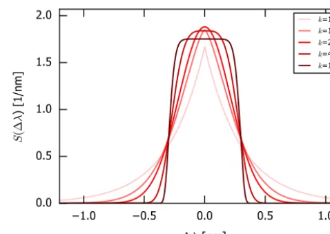
Figure 1 displaysSfor different values of the “shape pa-rameter”k. Fork=2,SequalsGwith
wk=2=
√
2σ. (4)
Fork >2,Sbecomes “flat-topped”, converging to a boxcar shape of width 2wfork→ ∞. Fork <2,Sbecomes more peaked at the top, with long tails on both sides.
The SG as defined in Eq. (2) is symmetric by definition but can easily be extended to an asymmetric SG (ASG) by intro-ducing asymmetry parameters forwand/ork, as described in Appendix A. In this study, we focus on symmetric SGSor the asymmetric extensionSaw with the additional parameter
awdetermining the asymmetry of its width (see Appendix A for details).
The full width at half maximum (FWHM), which is often used as measure for the width of a distribution, is
FWHM=2k
√
ln 2w, (5)
1.0
0.5
0.0
0.5
1.0
∆
λ
[nm]
0.0
0.5
1.0
1.5
2.0
S
(∆
λ
) [
1/
nm
]
k=1.0 k=1.5 k=2.0 k=4.0 k=10.0
Figure 1.Illustration of the “super-Gaussian” as defined in Eq. (2)
forw=0.3 nm and different values of the shape parameterk.
i.e., it depends onk. For the SG, it is thus useful to consider the “full width at 1/ethmaximum” (FWEM) instead, as this directly corresponds towdoubled:
FWEM=2w, (6)
which holds independent ofk, even in the asymmetric case (see Appendix A).
2.2 Parameterizing ISRF changes
Changes of the ISRF cause a spectral response to the mea-sured spectra. In particular for direct or scattered sunlight, this response is highly structured due to the Fraunhofer lines. Such spectral structures impair spectral analyses like DOAS, resulting in larger fit residuals, larger statistical errors of fit-ted column densities, and possibly also systematic biases if not appropriately accounted for.
In this section we show that the spectral structures caused by a change of the ISRF can be linearized with respect to the parameter change and thus can be accounted for by adding correction spectra to the spectral analysis. This generally makes the fit more stable, as local side minima are excluded, and significantly faster.
2.2.1 Change of ISRF
BeP (p)a general parameterization of the ISRF with param-eterp. In order to parameterize the effect ofchangesof p, we determine the Taylor expansion ofP around the baseline P∗=P (p∗)for a change of1p=p−p∗:
P (p, λ)=P (p∗, λ)+1p∂P (p, λ)
∂p |p
∗+O(2)
=P∗+1p×∂pP+O(2), (7)
with ∂pP :=
∂P (p, λ)
[AU]
0
ISRF and derivatives
S
[AU]
0
wS
1.0 0.5 0.0 0.5 1.0 ∆λ [nm]
[AU] 0
kS 0.1 0.2 0.3 0.4 0.5 0.6 0.7 0.8
0.9 Intensity space
I=S⊗˜I
0.6 0.4 0.2 0.0 0.2 0.4 0.6
Jw= wS⊗I˜
396 398 400 402 404
λ [nm]
0.02 0.01 0.00 0.01 0.02
Jk= kS⊗˜I 2.0 1.5 1.0 0.5 0.0 0.5 1.0 1.5
2.0 Optical depth space
ˆ
σw= wS⊗˜I/S⊗I˜
396 398 400 402 404
λ [nm]
0.08 0.06 0.04 0.02 0.00 0.02 0.04 0.06
ˆ
σk= kS⊗˜I/S⊗I˜
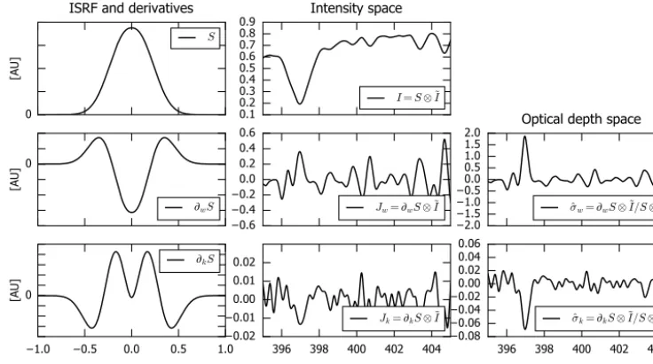
Figure 2.Illustration of the effect of ISRF changes on spectra in intensity and optical depth space. Left: super-GaussianSforw=0.3 nm
andk=2.3 (top) and its partial derivatives with respect tow(center) andk(bottom). Center: intensityI, derived from a high-resolution solar spectrum (Kurucz et al., 1984) by convolution withS(top), and the RCSJwandJkcaused by changes ofw(center) andk(bottom),
according to Eq. (12). Right: PAσˆ caused by changes ofw(center) andk(bottom) in optical depth, according to Eq. (19). The actual change of OD results after scaling with1w(in nm) and1k, respectively. For instance, a change of the ISRF width of1w=0.01 nm causes OD changes of about 5 ‰ up to 2 % around the strong calcium line at 396.85 nm.
denoting the partial derivative ofP with respect top, evalu-ated atp∗. For illustration, Fig. 2 (left) displaysP =Sand its partial derivatives with respect towandk.
Thus, the change ofP with respect to the baseline can be linearized:
1P :=P−P∗≈1p×∂pP . (9)
The error made by neglecting the nonlinear O(2)terms is quantified in Appendix C. As rule of thumb, linearization works well for relative parameter changes below 10 %. 2.2.2 Impact onI: resolution correction spectra (RCS) The ISRF describes the response to a monochromatic input. For a high-resolution input spectrumeI, the measured signal I results from the convolution ofeI with the ISRF:
I =P⊗eI . (10)
Consequently,
1I :=I−I∗=P ⊗eI−P ∗⊗
e I
=1P⊗eI≈1p×∂pP ⊗eI=1p×Jp (11)
describes the effect of changes ofP on the measured spec-trumI, expressed as the spectral structure
Jp=∂pP⊗eI , (12)
scaled by the parameter change1p. Below, we refer toJpas RCS. Figure 2 (center column) displaysJw andJkfor a SG parameterization.
In case of a wavelength-dependent ISRF,pcan be approx-imated to change linearly around a central wavelengthλc, wherep=pc:
p=pc+a×(λ−λc), (13)
and thus
1p=a×(λ−λc) . (14)
Consequently, the RCS
Jp,λ:=Jp×(λ−λc) , (15)
scaled bya (i.e., the change ofpper wavelength), reflects the spectral structures caused by a linear wavelength depen-dency of parameterp. Wavelength dependencies of higher order(λ−λc)n,n≥2 can be parameterized analogously if necessary. This approach allows for a simple implementa-tion of the wavelength dependency of the ISRF within wave-length calibration, as demonstrated in Sect. 5.2.
2.2.3 Impact on convolved cross sections
If RCS are included in the spectral calibration procedure (see Appendix B), the fit parameters ofJpdirectly yield the change1pof the ISRF parameterp. This can be used for an improved convolution of absorption cross sectioneσ: σ= S+1p∂pS
⊗
2.2.4 Impact on DOAS: pseudo-absorber
Within DOAS analysis, slant column densities (SCDs)s, i.e., concentrations integrated along the effective light path, of at-mospheric absorbers can be derived from the measured OD by solving
τ = −ln I I0
=X
i
siσi+5, (17)
whereσi is the absorption cross section of trace gasi, and 5is a closure polynomial in wavelength accounting for Mie and Rayleigh scattering as well as other low-frequency con-tributions. It is common practice to account for other effects beyond actual trace gas absorptions in a formally analogue way by including PAσˆi, i.e., spectral structures with phys-ical meaning and units different from real absorption cross sections, but applicable in the same mathematical formalism. Commonly used PA are a “Ring spectrum”, accounting for rotational Raman scattering, or an inverse intensity spectrum accounting for an intensity offset. Spectral shift and stretch can also be accounted for by PAs (Beirle et al., 2013).
Respective PAs can be defined in order to include the ef-fects of ISRF changes in DOAS analysis in a linearized way: In optical depth space, the respective change caused by 1p is
1τ =ln(I∗+1I )−ln(I∗)=ln
1+1I
I∗
≈1I
I∗ , (18) again illustrated forSin Fig. 2 (right).
Thus, the PA is defined as
ˆ
σp=
∂pP⊗eI
P⊗eI
, (19)
for an overall change ofp(compare Fig. 2), and as
ˆ
σp,λ=
∂pP⊗eI
P⊗eI
×(λ−λc) , (20)
for a wavelength-dependent change. Note that while RCSs are defined on high spectral resolution, PAs have to be sam-pled on the instrument’s wavelength grid in order to be in-cluded in DOAS analysis. In case of ISRF derivatives which are not resolved by the instrument, the respective PAs are un-dersampled.
The respective factorssˆi (“pseudo-SCDs”) in Eq. (17) di-rectly represent the change of the ISRF parameter 1p. By including the spectral patterns related to ISRF changes in DOAS analysis, fit quality improves (residuals are reduced), which generally reduces statistical as well as systematic er-rors of the derived trace gas SCDs, and is a prerequisite for the accurate retrieval of trace gases with low optical depths, such as glyoxal or HONO. In addition, the information on the ISRF change might be of interest in itself for diagnosis of the instrument’s state.
The above formalism allows for a unique definition of PAs by Eqs. (19) and (20) ifIeis taken from a high-resolution so-lar atlas, such as provided by Kurucz et al. (1984). Thereby the effects of additional trace gas absorptions in the mea-sured spectrum are neglected, which is justified as the spec-tral structures of all (direct or scattered) solar spectra are usu-ally by far dominated by the Fraunhofer lines. However, in case of absorbers with high optical depth, e.g., for ozone in the UV or water vapor in the red spectral range, the effect of ISRF changes (and thus the appropriate PA) depend on the OD of the trace gas of interest. This might be accounted for by, e.g., calculating various PA for different a priori OD, and determine the appropriate PA matching the measurement iteratively.
In this section, the impact of ISRF changes is derived gen-erally for any ISRF parameterizationP. The SGS, however, is particularly suited for this approach due to the limited number of parameters, i.e., PAs, and the tangible meaning of the parametersw (width) andk (shape) and, optionally, aw (asymmetry). The same would hold for a parameteriza-tion based on a measured ISRF tuned by, e.g., widening or sharpening parameters as in Sun et al. (2016), which might be preferable when high-quality pre-launch measurements of the ISRF of satellite instruments are available and analytical parameterizations do not meet accuracy requirements.
3 Datasets and instruments
In this section, we briefly describe the datasets and instru-ments used in this study. Further details are provided in the given references.
3.1 High-resolution solar atlas
A solar spectrum with high accuracy and high spectral res-olution is required for the calculation of RCS and PAs (pre-vious section) and the wavelength calibration as described in Appendix B. For this purpose, we use the solar atlas provided by Kurucz et al. (1984).
In order to limit computational costs (e.g., for the convo-lution with the ISRF), the original data were pre-convolved with a Gaussian ofσ =0.025 nm width and sampled on a regular 0.01 nm grid. We found no indication for system-atic effects on our results related to under-sampling. As the resulting spectrumeI is used for all following convolutions within this study, the resulting widthsware slightly biased low (as they miss the pre-convolution), but the effect is neg-ligible.
3.2 Avantes spectrometer
back-thinned Hamamatsu S11071-1106 detector. The instru-ment is similar to that described in Lampel et al. (2015).
The spectrometer is temperature stabilized (1T < 0.02◦C). The UV spectrometer covered a spec-tral range of 296–459 nm at a FWHM specspec-tral resolution of
≈0.55 nm (at 334 nm) or≈6 pixel. The spectral stability was typically better than ±3 pm per day and better than
±5 pm for the duration of the measurements from 23 April 2015 until 3 March 2016 at the Penlee Point Atmospheric Observatory on the southwest coast of the UK (e.g., Yang et al., 2016). No significant change of the ISRF, measured each night based on an Hg discharge lamp, was observed during the campaign.
3.3 GOME-2
GOME-2 on MetOp-A was launched in 2006 as first of three GOME-2 instruments, providing a multi-annual time series of spectral measurements of the light reflected by the Earth’s surface and atmosphere. The instrumental characteristics of GOME-2 are described in Callies et al. (2000) and Munro et al. (2016). The optical spectrometer covers the spectral range from 240 to 790 nm in four different channels. Spatial coverage is achieved by scanning the Earth via a scan mir-ror. The spectrometers have spectral resolutions (FWHM) of about 0.26 nm (UV) to 0.51 nm (VIS), with the ISRF usually parameterized by a Gaussian (Siddans et al., 2006; Munro et al., 2016).
GOME-2 spectral measurements are provided by EU-METSAT. In this study, we investigate the daily solar mea-surements from GOME-2 on MetOp-A for the years 2007– 2014, and Earth’s backscattered radiance for one arbitrarily chosen orbit on 1 April 2009.
3.4 OMI
OMI on AURA was launched in 2004 as part of the “A-train” (Levelt et al., 2006). It covers the spectral range from 270 to 500 nm in two spectral bands: the UV with a resolution of
≈0.42–0.45 nm FWHM and the VIS with a FWHM of about 0.63 nm.
OMI is operated in push-broom mode, i.e., the across-track dimension is measured simultaneously by a CCD instead of scanned consecutively by a mirror, as for GOME-2. This im-plies that different viewing angles have different instrument properties, i.e., ISRFs.
For OMI, the ISRF is significantly different from a sim-ple Gaussian, being more flat-topped (Dirksen et al., 2006). The operational parameterization of the OMI ISRF is thus composed of a Gaussian and a “broadened Gaussian”, which corresponds to a SG with a fixedk=4.
In this study, we use the solar irradiance climatology com-piled from daily OMI measurements in 2005.
3.5 TROPOMI/Sentinel 5 Precursor
TROPOMI will be launched in 2017 within the S-5P mis-sion (Veefkind et al., 2012). Its instrumental design is simi-lar to OMI, but TROPOMI provides higher spatial resolution and additional NIR and short-wave infrared (SWIR) chan-nels. The UV, UVIS, and NIR spectral bands cover the tral ranges 270–320, 320–490, and 710–775 nm, with spec-tral resolutions (FWHM) of 0.45–0.5, 0.45–0.65, and 0.34– 0.35 nm, respectively (A. Ludewig, personal communication, 2016). The SWIR spectral band covers the spectral range 2305–2385 nm with a FWHM of 0.25 nm (Veefkind et al., 2012).
The TROPOMI ISRF has been extensively measured on ground before launch based on various SLSs. Generally it was found to be extremely flat-topped for the UV below 310 nm, Gaussian to triangular for the UVIS (310–500 nm), flat-topped for the NIR, and slightly flat-topped for the SWIR.
Here we investigate the performance of the SG parameter-ization for sample TROPOMI ISRFs for each spectral chan-nel. The respective calibration measurements for UV, UVIS, and NIR are based on a slit function stimulus (SFS) con-structed by a monochromator using a rotating grating, and have been provided by Antje Ludewig and Joost Smeets from KNMI (personal communication, 2016). The SWIR calibra-tion measurements were performed with an optical paramet-ric oscillator (OPO) and have been provided by Paul Tol from SRON (personal communication, 2016).
4 Parameterizing the ISRF by a super-Gaussian In this section we investigate the performance of a super-Gaussian parameterization of the ISRF for different detectors and demonstrate its benefits compared to a simple Gaussian parameterization.
4.1 Avantes
Figure 3 displays the Hg line at 404.66 nm (left) and a zenith-sky spectrum (right) measured by the Avantes spectrometer described in Sect. 3.2 and the results of a least-squares fit of the ISRF parameterized as Gaussian,G(green), or super-Gaussian,S(orange). For the zenith-sky spectrum, the ISRF is fitted within the spectral calibration procedure, making use of the highly structured Fraunhofer lines (see Appendix B). The respective fit results are listed in Tables 1 and 2, and the residual of the wavelength calibration is shown in Fig. 3 (right bottom).
0.6 0.4 0.2 0.0 0.2 0.4 0.6 ∆λ [nm]
ISRF [AU]
Measured Gauss Super-G
0.0 0.2 0.4 0.6 0.8 1.0
Normalized intensity [AU]
Measured a-priori ISRF Gauss Super-G
400 402 404 406 408 410
λ [nm] 0.02
0.01 0.00 0.01 0.02
Residue
(a) (b)
Figure 3.ISRF fit results for Avantes. Left: measured (crosses) line shape of the Hg line at 404.66 nm and best matching parameterizations
GandS. Right: least-squares fit of the ISRF during wavelength calibration of a zenith-sky measurement in the 400–410 nm interval (top) and corresponding residual (bottom), with ISRF derived from the Hg measurement (“a priori”) or parameterized asGandS.
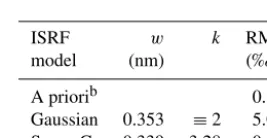
Table 1.Fit results of ISRF parameterized asGorSfor the Hg line
at 404.66 nm as measured by the Avantes spectrometer.
ISRF FWHM w k RMS
model (nm) (nm) (‰)∗
Gaussian 0.560 0.336 ≡2 31.10
Super-G. 0.620 0.348 3.15 6.77
∗Relative to maximum Hg.
0.353 nm for Hg fit and wavelength calibration, respectively, i.e., agrees within 5 % for both fits.
The flat-topped shape of the measured Hg line is much better reflected by the super-Gaussian parameterization with a shape parameterk=3.15, and the spectral calibration re-sults in much lower residuals (0.884 ‰ RMS for wavelength calibration). In addition, the performance of the wavelength calibration based onSis almost as good as had the measured Hg line been taken as ISRF directly. Again, the fitted param-eters of the direct ISRF fit and the wavelength calibration are consistent within 5 % for bothwandk(Tables 1 and 2).
The fittedw(and thus the FWEM) forGvs.Sare com-parable within 5 % as well. In contrast, the FWHM of the fitted ISRFs to the Hg line differ by more than 10 % between GandS(Table 1). The concept of FWHM, widely used due to historic reasons when distribution widths were determined graphically, thus seems to be a suboptimal measure for the width of the ISRF for non-Gaussian shapes. We thus focus onw(=1/2 FWEM) instead of FWHM hereafter.
4.2 GOME-2
For GOME-2, the ISRF is usually parameterized by a Gaus-sian (Siddans et al., 2006; Munro et al., 2016) or an asymmet-ric Gaussian (e.g., De Smedt et al., 2012). We have tested the benefit of a super-Gaussian parameterization over a
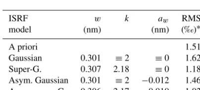
Gaus-Table 2.Fit results of ISRF parameterized asGorSfor the
wave-length calibration (400–410 nm) of the zenith-sky spectrum mea-sured by the Avantes spectrometer.
ISRF w k RMS
model (nm) (‰)a
A priorib 0.81
Gaussian 0.353 ≡2 5.00
Super-G. 0.339 3.28 0.88
aRelative to maximum intensity.bMeasured
Hg line, offset corrected and interpolated.
sian, both symmetric as well as asymmetric, exemplarily for a direct sun measurement on 23 January 2007. For the asym-metric parameterizations as defined in Eq. (A1), the asymme-try parameterawis included, allowing for different widths on both flanks of the ISRF (see Appendix A).
Figure 4 (left) displays the measured sun spectrum (black) and the results of the wavelength calibration for asymmetric GandSin the interval 420–440 nm. This wavelength range was chosen for comparison of the long-time evolution of the ISRF with Munro et al. (2016); see Sect. 5.1.1. The fitted asymmetric ISRFs are displayed in Fig. 4. For comparison, the operational ISRF from GOME-2 key data is included as well. Fit results (including symmetric parameterizations) are summarized in Table 3.
0.0 0.2 0.4 0.6 0.8 1.0
Normalized intensity [AU]
Measured a-priori ISRF Gauss Super-G
420 425 430 435 440
λ [nm] 0.02
0.01 0.00 0.01 0.02
Residue
0.6 0.4 0.2 0.0 0.2 0.4 0.6
∆λ [nm]
ISRF [AU]
(a) (b)
Figure 4.ISRF fit results for the GOME-2 direct sun measurement on 23 January 2007. Left: least-squares fit of the ISRF during wavelength
calibration in the 420–440 nm interval (top) and corresponding residual (bottom), with ISRF parameterized asGandSand the official ISRF (purple). Right: illustration of the best matching ISRF parameterizationsGandSand the official ISRF (purple).
Table 3.Fit results of ISRF parameterized asGorSfor the
wave-length calibration (420–440 nm) of the direct solar spectrum mea-sured by GOME-2.
ISRF w k aw RMS
model (nm) (nm) (‰)∗
A priori 1.51
Gaussian 0.301 ≡2 ≡0 1.62
Super-G. 0.307 2.18 ≡0 1.18
Asym. Gaussian 0.301 ≡2 −0.012 1.46
Asym. super-G. 0.306 2.17 −0.010 1.02
∗Relative to maximum intensity.
Avantes spectrometer (previous section) or OMI (next sec-tion). For the fit shown in Fig. 4, the use of an asymmetric super-Gaussian parameterization within wavelength calibra-tion improves the fit RMS to 1.02 ‰, compared to 1.46 and 1.51 ‰ for an asymmetric Gaussian parameterization and the ISRF from key data, respectively.
4.3 OMI
Figure 5 displays the wavelength calibration for the OMI sun climatology based on the official ISRF (at 430 nm) and pa-rameterization G andS. Fit results are summarized in Ta-ble 4.
Obviously, a parameterization of the ISRF by a Gaussian is not appropriate for OMI and results in a highly structured residual with 5.64 ‰ RMS. With the super-Gaussian parame-terization, residuals are significantly smaller (0.85 ‰ RMS). The operational OMI ISRF has been found to be asymmet-ric (Dirksen et al., 2006). However, for the asymmetasymmet-ric pa-rameterization,awwas found to be very small (−0.005 nm), the fitted ISRF hardly changes, and the fit residual hardly improves over the symmetricS(see Table 4). The fit results
Table 4.Fit results of ISRF parameterized asGorSfor the
wave-length calibration (420–440 nm) of the direct solar spectrum mea-sured by OMI.
ISRF w k aw RMS
model (nm) (nm) (‰)∗
A priori 2.29
Gaussian 0.336 ≡2 ≡0 5.64
Super-G. 0.362 3.44 ≡0 0.85
Asym. SG 0.362 3.44 −0.004 0.84
∗Relative to maximum intensity.
for S are still better (in terms of RMS) than those derived based on the operational ISRF (“a priori”) derived from pre-flight measurements. This might indicate a slight change of the ISRF after launch. However, the shape of a priori and SG ISRFs (in particular the flanks) is quite similar (see Fig. 5b). 4.4 TROPOMI/S-5P
We apply the super-Gaussian parameterization exemplarily to one set of SFS measurements for each TROPOMI detec-tor around the center row and column of the detecdetec-tor, corre-sponding to the central wavelength and nadir-viewing geom-etry. The ISRFs and best matching parameterizationsGand S are illustrated in Fig. 6. Note that at the detector center, TROPOMI ISRFs are quite symmetric. In Appendix A, also asymmetric samples from the detector edges are shown.
0.0 0.2 0.4 0.6 0.8 1.0
Normalized intensity [AU]
Measured a-priori ISRF Gauss Super-G
420 425 430 435 440
λ [nm] 0.02
0.01 0.00 0.01 0.02
Residue
0.6 0.4 0.2 0.0 0.2 0.4 0.6
∆λ [nm]
ISRF [AU]
(a) (b)
Figure 5.ISRF fit results for the OMI direct sun measurement climatology for cross-track pixel 2 (0-based). Left: least-squares fit of the
ISRF during wavelength calibration in the 420–440 nm interval (top) and corresponding residual (bottom), with ISRF parameterized asG andSand the official ISRF (purple). Right: illustration of the best matching ISRF parameterizationsGandSand the official ISRF (purple).
0.6 0.4 0.2 0.0 0.2 0.4 0.6 ∆λ [nm]
ISRF [AU]
k=7.4
Measured Gauss Super-G
0.6 0.4 0.2 0.0 0.2 0.4 0.6 ∆λ [nm]
ISRF [AU]
k=2.4
Measured Gauss Super-G
0.6 0.4 0.2 0.0 0.2 0.4 0.6 ∆λ [nm]
ISRF [AU]
k=3.0
Measured Gauss Super-G
0.6 0.4 0.2 0.0 0.2 0.4 0.6 ∆λ [nm]
ISRF [AU]
k =2.7
Measured Gauss Super-G
(a) (b) (c) (d)
Figure 6.Exemplary TROPOMI ISRF for the UV(a), UVIS(b), NIR(c), and SWIR(d)at the detector centers. Crosses indicate the
pre-launch measurements (provided by Antje Ludewig (UV, UVIS, NIR) and Paul Tol (SWIR), personal communication, 2016). Lines show the best matching parameterizationsGandS. The respective fit parameters are listed in Table 5.
Table 5.Fit results of ISRF parameterized asGorS for sample
TROPOMI pre-launch calibration measurements at detector center.
Detector ISRF w k RMS
model (nm) (‰)∗
UV Gaussian 0.237 ≡2 124.1
Super-G. 0.246 7.38 7.5
UVIS Gaussian 0.277 ≡2 21.1
Super-G. 0.284 2.39 15.4
NIR Gaussian 0.183 ≡2 28.2
Super-G. 0.191 3.03 4.2
SWIR Gaussian 0.126 ≡2 25.4
Super-G. 0.130 2.69 5.9
∗Relative to maximum intensity.
The official ISRF parameterizations (Antje Ludewig and Paul Tol, personal communication, 2016) are based on
– advanced sigmoids, involving nine parameters, for the UV and NIR;
– a “generalized exponential” with eight parameters for the UVIS; and
– the convolution of a skew-normal and a block distribu-tion, plus a Pearson VII distribudistribu-tion, for the SWIR, in-volving eight parameters in total.
param-eterization might not be sufficient for applications with high accuracy requirements.
5 Parameterizing changes of the ISRF by RCS and PA In the second part of the paper we present applications of the linearisation of ISRFchangesderived in Sect. 2.2. As stated therein, this concept might be applied to any ISRF param-eterization, but the SG is particularly useful due to the low number of parameters and their illustrative meaning.
In Sect. 5.1 we investigate changes of the ISRF over time, i.e., long-term as well as in-orbit changes, exemplarily for GOME-2.2
In Sect. 5.2 we demonstrate the concept of considering the wavelength dependency of the ISRF by RCS.
5.1 Changes of the ISRF over time
5.1.1 Long-term changes of the GOME-2 ISRF
Munro et al. (2016) have shown that the GOME-2 ISRF changes over time, in particular for the UV and blue spec-tral range. Figure 10 in Munro et al. (2016) shows that the FWHM of a Gaussian fitted to SLS measurements during daily calibration decreases by about 5 % from 2007 to 2010 at 429 nm. In addition, the FWHM reveals a seasonal pattern. Munro et al. (2016) have related this temporal pattern of the GOME-2 ISRF to the optical bench temperature and found good correlation.
We investigate the temporal evolution of the GOME-2 ISRF width around 429 nm by performing wavelength cal-ibration fits for the daily solar spectra for four different fit settings:
1. The ISRF is fitted as Gaussian, as in Munro et al. (2016). 2. The ISRF is fitted as super-Gaussian.
3. The ISRF is fixed to the results of setting 2 for the first day of the time series.
4. As in setting 3 but, in addition, the RCSJwandJk, de-rived from Taylor expansion, are included in the fit (see Eq. 12).
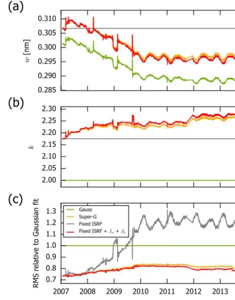
Figure 7 displays the time series of fit results forw,k, and the fit RMS (relative to the Gaussian fit).
1. The first evaluation reproduces the findings shown in Munro et al. (2016): the ISRF width decreases from 2007 to the end of 2009, when the detector was heated during throughput tests. Afterwards, seasonal variations dominate on top of a constant level. Note that the time series shown in Fig. 7 and in Fig. 10 in Munro et al. 2For OMI (not shown), we could not find indications for a
sig-nificant change of the ISRF over time.
0.285 0.290 0.295 0.300 0.305 0.310
w
[n
m]
(a)
2.00 2.05 2.10 2.15 2.20 2.25 2.30
k
(b)
2007 2008 2009 2010 2011 2012 2013 2014
Year
0.7 0.8 0.9 1.0 1.1 1.2 1.3
RMS relative to Gaussian fit
(c)
Gauss Super-G Fixed ISRF Fixed ISRF + Jw + Jk
Figure 7.Temporal evolution of the GOME-2 ISRF fitted for daily
solar measurements (420–440 nm) for four fit settings, i.e., a Gaus-sian parameterization (green), a super-GausGaus-sian parameterization (orange), a fixed ISRF matching the super-Gaussian from the first day (grey), and a fixed ISRF plus the RCSJw andJk (red). The
subplots display the fitted width(a), shape(b), and fit RMS relative to the Gaussian fit(c).
(2016) agree well within a surprising level of detail, though the latter was derived from calibration measure-ments, while the first is based on solar measurements. 2. The results of the SG fit have already been discussed
in Sect. 4.2 for the first day of the time series: the SG slightly improves the fit residual and yields a shape pa-rameter slightly above 2 (k=2.17). The temporal evo-lution ofw is similar to that for the Gaussian fit, but shifted by about 0.005 nm. Interestingly, the fittedkalso shows a clear temporal pattern, increasing by about 0.1 over the time series; i.e., not only thewidth, but also the shapeof the GOME-2 ISRF has changed.
4. In setting 4, the ISRF is kept constant as well, as for setting 3, but the effect of ISRF changes is accounted for by including the RCSJw andJk in the wavelength calibration procedure. Time-dependent values forwand kare thus derived from the values of the a priori ISRF plus the respective RCS fit coefficients. Resultingwand kagree very well with setting 2, and the fit RMS for set-ting 4 is even lower than for setset-ting 2. The explanation for this, at first glance unexpected, finding is that the GOME-2 ISRF, though well approximated byS, is not an exact super-Gaussian. The fit settings 2 and 4 span two slightly different groups of ISRF shapes, and set-ting 4 is slightly better represenset-ting the actual GOME-2 ISRF.
Thus, while the application of a fixed ISRF for the GOME-2 time series begins to become suboptimal after GOME-2 years, the additional inclusion of RCS actually accounts for the spectral changes caused by the ISRF changes over time.
5.1.2 In-orbit changes
The case study shown above illustrates that the linearisation of ISRF changes generally works; however, a full ISRF fit might easily be performed for each daily measured sun ref-erence instead. This is different if the ISRF changes along orbit: due to the high number of spectra, a full fit of the ISRF is not feasible any more. Thus, in the case of trace gas retrievals, the concept of linearisation by accounting for changes by a PA, which can be included in a linear fit setup, is highly beneficial.
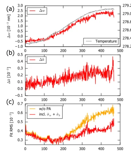
We have investigated the benefit of the PAσˆw for a sam-ple fit in the visible spectral range for one orbit measured by GOME-2 A. Figure 8a displays the fit parameter1w, which directly reflects the in-orbit change of the ISRF widthw. A similar effect has been shown by Azam and Richter (2015, Fig. 23 therein), who derived the ISRF for each individual satellite pixel by a nonlinear fit of the solar atlas.
The systematic change of ISRF width along orbit is closely related to the temperature of the pre-disperser prism (Fig. 8a). Thus, the fit parameter of the fitted PAσˆwdirectly serves as a diagnostic tool for the instrument’s state.
The respective change of the fitted shape parameter k is shown in Fig. 8b. While significantly increasing, the effect is negligibly small.
Figure 8c displays the fit RMS for retrievals with and with-out both σˆw andσˆk. The inclusion of the PA significantly improves the fit and removes a systematic component of the residual, which is a prerequisite for improved trace gas anal-yses, in particular for trace gases with low OD.
5.2 Changes of ISRF over wavelength
The ISRF generally depends on wavelength. In Sect. 2.2, it is shown that the spectral structure caused by ISRF changes over wavelength can be linearized as well. In this
0 100 200 300 400 500 1.0
0.5 0.0 0.5 1.0 1.5 2.0 2.5 3.0
∆
w
[1
0
−
3 n
m]
(a)
∆w278.2 278.4 278.6 278.8 279.0 279.2
T [K]
Temperature
0 100 200 300 400 500 0.1
0.0 0.1 0.2 0.3 0.4 0.5
∆
k
[1
0
−
3]
(b)
∆k
0 100 200 300 400 500 Scan no.
0.3 0.4 0.5 0.6 0.7
Fit
R
MS
[1
0
−
3]
(c)
w/o PA incl. ˆσw + ˆσk
Figure 8.Temporal change of the GOME-2 ISRF along orbit on
1 April 2009 as derived from a linear fit including the PAsσˆw and
ˆ
σk. Top: in red, the fit results for 1ware shown, indicating the
change of the ISRF width. Fit results are averaged over one full GOME-2 scan (24 forward and 8 backscan pixels). In grey, the tem-perature of the predisperser prism, as provided in the operational lv2 files, is shown. Center: fit results for1kaveraged over one scan. Bottom: fit RMS (based on residuals averaged over one scan) com-pared for retrievals with and without PA.
section, we demonstrate this concept for a synthetic spec-trum (Sect. 5.2.1) as well as actual GOME-2 measurements (Sect. 5.2.2).
5.2.1 Proof of concept: synthetic spectrum
We construct a synthetic spectrum by convolution ofeI with a wavelength-dependent ISRF withwincreasing linearly by 0.003 nm nm−1, i.e., from 0.27 nm (at 420 nm) to 0.33 nm (at 440 nm). The ISRFs and the resulting spectrum are illustrated in Fig. 9.
In Fig. 10, the wavelength calibration results are shown for (a) a simple SG parameterization with wavelength-independent ISRF (orange) and (b) additional inclusion of the RCSJw,λ=Jw×(λ−λc).
439 440 441
//
w
=0.33
429 430 431
λ [nm]
//
w
=0.30
w=const. w=w(λ)419 420 421
ISRF / normalized intensity [AU]
w
=0.27
Figure 9.Illustration of the generation of a synthetic spectrum in order to investigate wavelength-dependent ISRF changes. In black, the
result ofI=S⊗eI, based on the ISRFS(w=0.3, k=2.2), is shown. In red, the respectiveIfor the wavelength-dependent ISRF is shown
with1w=0.03 nm nm−1.
0.0
0.2
0.4
0.6
0.8
1.0
Normalized
intensity [AU]
Synth. spectrum Super-G
Super-G+Jw, λ
420
425
430
435
440
λ
[nm]
0.02
0.01
0.00
0.01
0.02
Residue
Figure 10.Fit results for the synthetic spectrum based on an ISRF
fit with the spectral structureJw,λexcluded (orange) and included
(cyan).
If the RCS Jw,λ is included in the fit, the synthetic spectrum can be reproduced almost perfectly with a fit RMS of 0.18 ‰, and the fitted change of w over wave-length (0.00297 nm nm−1) is very close to the a priori (0.003 nm nm−1).
5.2.2 Application: GOME-2
In this section, we apply the concept of RCS for describ-ing the ISRF wavelength dependency for GOME-2 measure-ments in the UV. We have determined the wavelength de-pendency of the ISRF, parameterized as Saw, by perform-ing wavelength calibrations in small (10 nm wide) fit win-dows (“subwinwin-dows”) in steps of 5 nm. A similar procedure is used in QDOAS (Danckaert et al., 2015) in order to deter-mine wavelength dependencies of ISRF width and spectral shifts. Figure 11 displays the resulting parametersw,k, and awas derived for the solar irradiance measured on 23 January 2007. The ISRF width of GOME-2 in the UV is generally de-creasing with wavelength, the shape is approximately
Gaus-330 340 350 360 370
0.145 0.150 0.155 0.160 0.165 0.170 0.175 0.180 0.185
w
[n
m]
RCS Sub-window fits
330 340 350 360 370
1.85 1.90 1.95 2.00 2.05 2.10 2.15 2.20
k
330 340 350 360 370
λ [nm] 0.040
0.035 0.030 0.025 0.020 0.015 0.010 0.005 0.000 0.005
a
w[n
m]
(a)
(b)
(c)
Figure 11.Wavelength dependency of the GOME-2 ISRF width
w(a), shapek(b), and asymmetryaw (c), as derived from SG fits
in subwindows of 10 nm width, sampled in 5 nm steps (black), and from the fit factors of the respective RCSJw,λ, Jk,λ, andJaw,λ
(red).
sian (k≈2) with increasingk, and the asymmetry parameter is negative for low wavelengths (meaning that the left flank of the ISRF is less steep than the right flank), increasing to-wards 0 (symmetry) at 375 nm.
RCS Jw,λ,Jk,λ, and Jaw,λ. The respective wavelength de-pendency ofw,k, andawas determined by the RCS fit coef-ficients is included in Fig. 11 in red, showing generally good agreement to the subwindow fit results.
Figure 12 displays the respective fit of the solar irradiance, again for fit settings excluding or including RCS. As for the synthetic case study, including RCS significantly improves the fit results, particularly at the edges of the fit window.
Thus, the wavelength dependency of the ISRF can be ac-counted for by including RCS in the wavelength calibration procedure, while the actual convolution S⊗eI is done for a constant ISRF, which is by far faster and more stable than actually fitting a wavelength-dependent ISRF.
6 Conclusions
The super-Gaussian is a powerful extension of the Gaussian which allows to represent a variety of different shapes by adding just one free shape parameterk, in addition tow de-scribing its width. Optionally, asymmetry can be described by a further asymmetry parameteraw. The super-Gaussian is particularly well suited for describing flat-topped ISRFs, as occur for OMI or TROPOMI (UV). Due to the low number of parameters, which are uncorrelated, the SG can be fitted within wavelength calibration of measurements of direct or scattered sunlight, making use of the highly structured Fraun-hofer lines, which is generally challenging for sophisticated ISRF parameterizations with many parameters.
Changes of the ISRF over time or wavelength can be ac-counted for by including spectral structures derived from the linear term of a Taylor expansion. In intensity and OD space, RCS and PAs are defined to be included in spectral cali-bration and DOAS analysis, respectively. The linearization makes the spectral analysis robust and fast; thus the inclu-sion of RCS and PA comes without notable performance loss. While this approach is possible for any ISRF parameteriza-tion, the SG is particularly suited due to the low number of parameters and the illustrative meaning of its parameters.
For GOME-2, the inclusion of PAs significantly improves the fit quality and removes a systematic component of the residual along orbit, as it appropriately accounts for the ef-fects of ISRF broadening along orbit. The fitted change of ISRF width directly corresponds to temperature. Generally, including RCS and PAs allows for easy monitoring of the long-term stability of an instrument by straightforward fit pa-rameters.
0.0
0.2
0.4
0.6
0.8
1.0
Normalized
intensity [AU]
Measured Super-G (asym. w)
SG+Jw, λ+Jk, λ+Jaw, λ
330
340
350
360
370
λ
[nm]
0.02
0.01
0.00
0.01
0.02
Residue
Figure 12.Fit result of the ISRF excluding (orange) or including
(cyan) RCS for the solar spectrum of GOME-2 on 23 January 2007 in the UV.
Accounting for the wavelength dependency of the ISRF by the proposed linearisation allows for considering wide fit-ting windows during spectral calibration and is thus a fast and robust alternative for the “subwindow” approach as im-plemented in QDOAS (Danckaert et al., 2015) or fitting a polynomial forw(λ)as in DOASIS (Lehmann et al., 2008).
7 Data availability
Appendix A: Implementation of the asymmetric super-Gaussian
The super-Gaussian as defined in Eq. (2) is symmetric inx, while an ISRF might generally be asymmetric. For the case of a Gaussian, several implementations of asymmetric shapes have been proposed which basically use different values for σ of the left and the right wing. Here, we follow a similar approach in order to allow for ASGs:
Sasym(x)=Aasym×
exp
−| x
w−aw
|k−ak
forx≤0 exp
−| x
w+aw
|k+ak
forx >0 ,
(A1) with the additional asymmetry parameters aw and ak. For aw=ak=0, this becomes Eq. (2). For ak=0, i.e., an ASG with asymmetric width, but symmetric shape parameter, we define
Saw:=Sasym,ak=0. (A2)
Figure A1 displays examples of the ASG for different param-eter settings.
Note that by this implementation of asymmetry, the FWEM ofSstill equals 2windependent of all other param-eters (as opposed to, e.g., a parameterization based on two width parameterswleft andwright). This aspect is more than a sophisticated detail, as it implies that the ASG parameters are almost uncorrelated and allows for a multi-step proce-dure: within a first step,wandkmight be estimated from a SG fit; in a second step, the asymmetry parameters can be optimized, while the values of w and k from the first step hardly change.
For an asymmetric function, the first moment (“center of mass”, COM) is generally not 0 any more. Consequently, the application of such an asymmetric ISRF would cause a net spectral shift in the measured spectrum. However, the effect of a possible spectral shift is usually accounted for during spectral calibration and should not interfere with the asym-metry of the ISRF. In order to separate both effects, we de-mand that the ISRF does not cause a shift; i.e., after calculat-ing the ASG accordcalculat-ing to Eq. (A1), the COM is determined, and the ASG is shifted accordingly and normalized to an in-tegral of 1. Figure A2 shows the ISRFs resulting from the shifted ASG shown in Fig. A1.
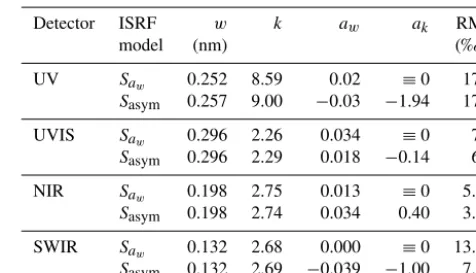
In Fig. A3, sample ISRFs from the different TROPOMI detectors and fitted ASG are shown with varying level of asymmetry. Table A1 lists the respective fit results.
The combined variation ofakandawcan lead to quite ex-otic shapes. For some instruments (in particular some Mini-MAX DOAS instruments, or the sample TROPOMI ISRF in the SWIR), this helped to slightly improve the fit perfor-mance for a direct ISRF measurement; however, within spec-tral calibration, the additional variety of possible shapes in-troduced by ak often results in unstable and diverging fits.
Table A1.Fit results of ISRF parameterized asGorSfor sample
TROPOMI pre-launch calibration measurements at detector edge.
Detector ISRF w k aw ak RMS
model (nm) (‰)∗
UV Saw 0.252 8.59 0.02 ≡0 17.9
Sasym 0.257 9.00 −0.03 −1.94 17.2
UVIS Saw 0.296 2.26 0.034 ≡0 7.0
Sasym 0.296 2.29 0.018 −0.14 6.9
NIR Saw 0.198 2.75 0.013 ≡0 5.68
Sasym 0.198 2.74 0.034 0.40 3.97
SWIR Saw 0.132 2.68 0.000 ≡0 13.73
Sasym 0.132 2.69 −0.039 −1.00 7.82
∗Relative to maximum intensity.
Within this study, we thus focus onSawfor wavelength cali-bration fits.
Appendix B: Wavelength calibration
The wavelength calibration of a spectrometer can be per-formed based on monochromatic stimuli with known wave-length, such as SLSs. However, as the instrument characteris-tics generally slightly changes during operation, an a posteri-ori wavelength calibration might be necessary. Within DOAS analysis, wavelength calibration is thus often done based on measured spectra of direct or scattered sunlight, making use of the highly structured Fraunhofer lines. Within this proce-dure, both the wavelength grid and a parameterized ISRF of the detector can be determined simultaneously.
In the following, we indicate spectral data with high res-olution with the tilde symbol. We model a high-resres-olution spectrum of direct or scattered sunlight by the function
e M(λ):
e
M(λ)=K(λ)e ×A(λ)e ×5emul(λ)+R(λ)e +e5add(λ). (B1)
e
K(λ)is the solar irradiance. A(λ)e =e− P
cj×eσj(λ)describes absorption by relevant atmospheric gases (like ozone) by Lambert–Beers law. R(λ)e accounts for rotational Raman scattering. Any other broadband features such as Mie and Rayleigh scattering, absolute scaling, and offsets are ac-counted for by the multiplicative and additive polynomials e
5mul and e5add. In case of direct irradiance measurements from satellite, the model function can be simplified as atmo-spheric absorption and scattering can be omitted. Note that wavelength calibration might as well be performed in terms of optical depths.
1.0 0.5 0.0 0.5 1.0
∆λ [nm]
[AU]
w
=0.3,
k
=2.5
aw=0.00
aw=0.06
aw=0.12
aw=0.18
1.0 0.5 0.0 0.5 1.0
∆λ [nm]
[AU]
w
=0.3,
k
=2.5
ak=0.00
ak=0.50
ak=1.00
ak=1.50
Figure A1.Illustration of the asymmetric super-GaussianSasymas defined in Eq. (A1) forw=0.3 nm,k=2.5, and different values for the
asymmetry parametersaw(left) andak(right).Aasymwas set to 1; i.e., the shown ASGs are not yet normalized.
1.0 0.5 0.0 0.5 1.0
∆λ [nm]
[AU]
w
=0.3,
k
=2.5
aw=0.00
aw=0.06
aw=0.12
aw=0.18
1.0 0.5 0.0 0.5 1.0
∆λ [nm]
[AU]
w
=0.3,
k
=2.5
ak=0.00
ak=0.50
ak=1.00
ak=1.50
Figure A2.ISRFs based on theSasymshown in Fig. A1; i.e.,Sasymis shifted such that the center of mass of the ISRF is 0, and normalization
is done empirically based on the interval [−2, 2] nm.
0.6 0.4 0.2 0.0 0.2 0.4 0.6 ∆λ [nm]
ISRF [AU]
Measured Super-G(asym. w) Super-G(asym. w and k)
0.6 0.4 0.2 0.0 0.2 0.4 0.6 ∆λ [nm]
ISRF [AU]
Measured Super-G(asym. w) Super-G(asym. w and k)
0.6 0.4 0.2 0.0 0.2 0.4 0.6 ∆λ [nm]
ISRF [AU]
Measured Super-G(asym. w) Super-G(asym. w and k)
0.6 0.4 0.2 0.0 0.2 0.4 0.6 ∆λ [nm]
ISRF [AU]
Measured Super-G(asym. w) Super-G(asym. w and k)
(a) (b) (c) (d)
Figure A3.Exemplary TROPOMI ISRF for the UV(a), UVIS(b), NIR(c), and SWIR(d)at the detector edges. Crosses indicate the
Sect. 2.2):
M(i)=(S⊗M)(λe i)+1p×Jp. (B2)
For a measured spectrumI (i)with the a priori wavelength gridλ∗i, the differenceM(i)−I (i)is minimized (“fitted”) by a nonlinear least-squares algorithm (here: using the python LMFit module by Newville et al., 2014), where the cali-brated wavelength grid λi is determined from the a priori wavelength gridλ∗by a linear transformation (allowing for spectral shift and stretch).
Fitted parameters are as follows:
– parameters ofS(justwin case of classical Gaussian,w andkin case of SG, andaw in case of asymmetry; see Appendix A);
– column densitiescj of the relevant absorbers included inA;
– intensity of Raman scattered lightR; – polynomial coefficients forPmulandPadd; – the RCS fit coefficients1p;
– shift and stretch of the wavelength grid transformation. The resulting calibrated wavelength grid and best-matching ISRF are used to provide the relevant cross sec-tions, necessary for a subsequent DOAS analysis, on the in-strument’s spectral resolution:
σj(i)=(S⊗eσj)(λi).
Based on the ISRF change1p determined during wave-length calibration, the convolution of cross sections can be corrected accordingly:
σj(i)= (S+1p∂pS)⊗eσj
(λi).
Appendix C: Error of Taylor expansion
In Sect. 2.2, the effects of ISRF changes are linearized based on a Taylor expansion, where terms of orderO(2)are omit-ted. We investigate the impact of this approximation for syn-thetic spectra for typical ISRF settings, i.e.,w0=0.3 nm and k=2.3. For a set of a priori changes ofw, spectra are derived by convolving the solar atlas with a super-Gaussian ISRF withw=w0+1w. Subsequently, a spectral calibration fit is performed for a fixed ISRF withw=w0, but includingJw in order to account for the change of ISRF width by lineariza-tion.
10-4 10-3 10-2 10-1
10-4
10-3
10-2
10-1
Fit
te
d
∆
w
[n
m]
1:1 Fit of Jw
10-4 10-3 10-2 10-1
True ∆w [nm] 10-10
10-9
10-8
10-7
10-6
10-5
10-4
10-3
Fit RMS
Figure C1.Errors induced by the linearization as investigated for
synthetic spectra with width w=0.3 nm+1w. Top: change of width1w, as fitted based onJw, versus the true change ofw.
Bot-tom: fit RMS in dependency of the true change ofw.
Figure C1 displays the results of this case study. In the top panel, the fitted1w, i.e., the fit coefficient ofJw, is displayed versus the a priori (“true”) change1w. In the bottom panel, the respective RMS of the spectral calibration fit is shown.
The Supplement related to this article is available online at doi:10.5194/amt-10-581-2017-supplement.
Competing interests. The authors declare that they have no conflict
of interest.
Acknowledgements. We would like to thank Andreas Richter (IUP
Bremen, Germany), Michel van Roozendael (BIRA Brussels, Belgium), Alexander Cede (LuftBlick, Austria), Antje Ludewig (KNMI, de Bilt, the Netherlands), Paul Tol (SRON, Utrecht, the Netherlands), and Kang Sun (Smithsonian Center for Astrophysics, Harvard, Cambridge, MA, USA) for helpful discussions on the topic of ISRF and the parameterization of its change.
Steffen Dörner and Jan Zörner from MPIC Mainz are acknowl-edged for helpful discussions on Python.
We thank Mingxi Yang from Plymouth Marine Laboratory for setting up and operating the EnviMeS/Avantes MAX-DOAS instru-ment at Penlee Point.
R. L. Kurucz is acknowledged for providing the solar atlas. GOME-2 spectral measurements are provided by EUMET-SAT, Darmstadt. OMI spectral measurements are provided by NASA. TROPOMI ISRF sample measurements are provided by Antje Ludewig and Joost F. C. Smeets (KNMI, de Bilt, the Netherlands) for UV/UVIS/NIR, and by Paul Tol (SRON, Utrecht, the Netherlands) for SWIR. This research was supported by the FP7 project QA4ECV, grant no. 607405.
The article processing charges for this open-access publication were covered by the Max Planck Society.
Edited by: M. Weber
Reviewed by: two anonymous referees
References
Azam, F. and Richter, A.: GOME2 on MetOp: Follow-on analysis of GOME2 in orbit degradatiFollow-on, Final
re-port, EUM/CO/09/4600000696/RM, 2015, available at:
http://www.doas-bremen.de/reports/gome2_degradation_ follow_up_final_report.pdf (last access: 7 September 2016), 2015.
Beirle, S., Sihler, H., and Wagner, T.: Linearisation of the effects of spectral shift and stretch in DOAS analysis, Atmos. Meas. Tech., 6, 661–675, doi:10.5194/amt-6-661-2013, 2013.
Callies, J., Corpaccioli, E., Eisinger, M., Hahne, A., and Lefebvre, A.: GOME-2 – Metop’s second-generation sensor for operational ozone monitoring, ESA Bull.-Eur. Space, 102, 28–36, 2000. Cede, A.: Manual for Pandora Software Suite, Version 1.6, 2013,
available at: http://avdc.gsfc.nasa.gov/pub/tools/Pandora/install/ (last access: 20 September 2016), 2013.
Cede, A.: Manual for Blick Software Suite 1.2, 2017, available at: http://pandonia.net/media/documents/BlickSoftwareSuite_ Manual_v6.pdf, last access: 14 February 2017.
Danckaert, T., Fayt, C., van Roozendael, M., de Smedt, I., Letocart, V., Merlaud, A., and Pinardi, G.: QDOAS Software user man-ual, available at: http://uv-vis.aeronomie.be/software/QDOAS/ QDOAS_manual.pdf (last access: 9 September 2016), 2015. Decker, F.: Beam distributions beyond RMS, in: Beam
Instrumen-tation Workshop, edited by: Mackenzie, G. H., Rawnsley, B., and Thomson, J., 550–556, Aip Press, Woodbury, USA, 1995. de Graaf, M., Sihler, H., Tilstra, L. G., and Stammes, P.: How
big is an OMI pixel?, Atmos. Meas. Tech., 9, 3607–3618, doi:10.5194/amt-9-3607-2016, 2016.
De Smedt, I., Van Roozendael, M., Stavrakou, T., Müller, J.-F., Lerot, C., Theys, N., Valks, P., Hao, N., and van der A, R.: Im-proved retrieval of global tropospheric formaldehyde columns from GOME-2/MetOp-A addressing noise reduction and instru-mental degradation issues, Atmos. Meas. Tech., 5, 2933–2949, doi:10.5194/amt-5-2933-2012, 2012.
Dirksen, R., Dobber, M., Voors, R., and Levelt, P.: Prelaunch characterization of the Ozone Monitoring Instrument transfer function in the spectral domain, Appl. Optics, 45, 3972–3981, doi:10.1364/ao.45.003972, 2006.
Fleck, J., Morris, J., and Feit, M.: Time-Dependent Propagation of High-Energy Laser-Beams Through Atmosphere, Appl. Phys., 14, 99–115, doi:10.1007/BF00882638, 1977.
Kurucz, R. L., Furenlid, I., Brault, J., and Testerman, L., Solar flux atlas from 296 to 1300 nm, in: National Solar Observatory At-las, Sunspot, National Solar Observatory, Sunspot, New Mexico, USA, 1984.
Lampel, J., Frieß, U., and Platt, U.: The impact of vibra-tional Raman scattering of air on DOAS measurements of at-mospheric trace gases, Atmos. Meas. Tech., 8, 3767–3787, doi:10.5194/amt-8-3767-2015, 2015.
Lehmann, T.: DOASIS Tutorial, available at: https:
//doasis.iup.uni-heidelberg.de/bugtracker/projects/doasis/ files/doasis_tutorial.pdf (last access: 9 September 2016), 2008. Levelt, P., Van den Oord, G., Dobber, M., Malkki, A., Visser, H.,
de Vries, J., Stammes, P., Lundell, J., and Saari, H.: The Ozone Monitoring Instrument, IEEE T. Geosci. Remote, 44, 1093– 1101, doi:10.1109/TGRS.2006.872333, 2006.
Liu, C., Liu, X., Kowalewski, M. G., Janz, S. J., González Abad, G., Pickering, K. E., Chance, K., and Lamsal, L. N.: Characterization and verification of ACAM slit functions for trace-gas retrievals during the 2011 DISCOVER-AQ flight campaign, Atmos. Meas. Tech., 8, 751–759, doi:10.5194/amt-8-751-2015, 2015. Miles, G. M., Siddans, R., Kerridge, B. J., Latter, B. G., and
Richards, N. A. D.: Tropospheric ozone and ozone profiles re-trieved from GOME-2 and their validation, Atmos. Meas. Tech., 8, 385–398, doi:10.5194/amt-8-385-2015, 2015.
Munro, R., Lang, R., Klaes, D., Poli, G., Retscher, C., Lind-strot, R., Huckle, R., Lacan, A., Grzegorski, M., Holdak, A., Kokhanovsky, A., Livschitz, J., and Eisinger, M.: The GOME-2 instrument on the Metop series of satellites: instrument de-sign, calibration, and level 1 data processing – an overview, At-mos. Meas. Tech., 9, 1279–1301, doi:10.5194/amt-9-1279-2016, 2016.
Nadarajah, S.: A generalized normal distribution, J. Appl. Stat., 32, 685–694, doi:10.1080/02664760500079464, 2005.
Ozone Monitoring Instrument (OMI): Data User’s Guide, available at: http://disc.sci.gsfc.nasa.gov/Aura/additional/documentation/ README.OMI_DUG.pdf (last access: 20 December 2016), 2012.
Platt, U. and Stutz, J.: Differential Optical Absorption Spec-troscopy, Springer-Verlag Berlin Heidelberg, Germany, 2008. Siddans, R., Kerridge, B. J., Latter, B.G., Smeets, J., and
Otter, G.: Analysis of GOME-2 Slit function
Mea-surements, Algorithm Theoretical Basis Document,
available at: ftp://ftp.eumetsat.int/pub/EPS/out/GOME/
Calibration-Data-Sets/Slit-Function-Key-Data/FM3-Metop-A/
g2_slit_function_analysis_atbd_v2p0.pdf (last access: 14
February 2017), 2006.
Sihler, H., Lübcke, P., Lang, R., Beirle, S., de Graaf, M., Hörmann, C., Lampel, J., Penning de Vries, M., Remmers, J., Trollope, E., Wang, Y., and Wagner, T.: In-operation Field of view Retrieval (IFR) for satellite and ground-based DOAS-type instruments ap-plying coincident high-resolution imager data, Atmos. Meas. Tech. Discuss., doi:10.5194/amt-2016-218, in review, 2016. Sun, K., Liu, X., Nowlan, C. R., Cai, Z., Chance, K., Frankenberg,
C., Lee, R. A. M., Pollock, R., Rosenberg, R., and Crisp, D.: Characterization of the OCO-2 instrument line shape functions using on-orbit solar measurements, Atmos. Meas. Tech. Discuss., doi:10.5194/amt-2016-335, in review, 2016.
Van Roozendael, M., De Smedt, I., Lerot, C., and Theys, N.: Trace gas products at BIRA-IASB Presentation given at the 50th GOME Science Advisory Group Meeting, EUMETSAT, 26– 27 November 2014, Darmstadt, Germany, 2014.
Veefkind, J. P., Aben, I., McMullan, K., Förster, H., de Vries, J., Otter, G., Claas, J., Eskes, H. J., de Haan, J. F., Kleipool, Q., van Weele, M., Hasekamp, O., Hoogeveen, R., Landgraf, J., Snel, R., Tol, P., Ingmann, P., Voors, R., Kruizinga, B., Vink, R., Visser, H., and Levelt, P. F.: TROPOMI on the ESA Sentinel-5 Precursor: A GMES mission for global observations of the atmospheric composition for climate, air quality and ozone layer applications, Remote Sens. Environ., 120, 70–83, doi:10.1016/j.rse.2011.09.027, 2012.
Yang, M., Bell, T. G., Hopkins, F. E., Kitidis, V., Cazenave, P. W., Nightingale, P. D., Yelland, M. J., Pascal, R. W., Prytherch, J., Brooks, I. M., and Smyth, T. J.: Air–sea fluxes of CO2and CH4