www.atmos-meas-tech.net/9/4079/2016/ doi:10.5194/amt-9-4079-2016
© Author(s) 2016. CC Attribution 3.0 License.
Proposed standardized definitions for vertical resolution and
uncertainty in the NDACC lidar ozone and temperature
algorithms – Part 3: Temperature uncertainty budget
Thierry Leblanc1, Robert J. Sica2, Joanna A. E. van Gijsel3, Alexander Haefele4, Guillaume Payen5, and Gianluigi Liberti6
1Jet Propulsion Laboratory, California Institute of Technology, Wrightwood, CA 92397, USA 2Department of Physics and Astronomy, The University of Western Ontario, London, Canada 3Royal Netherlands Meteorological Institute (KNMI), Bilthoven, the Netherlands
4Meteoswiss, Payerne, Switzerland
5Observatoire des Sciences de l’Univers de La Réunion, CNRS and Université de la Réunion (UMS3365), Saint Denis de la Réunion, France
6ISAC-CNR, Via Fosso del Cavaliere 100, 00133, Rome, Italy
Correspondence to:Thierry Leblanc (thierry.leblanc@jpl.nasa.gov)
Received: 6 April 2016 – Published in Atmos. Meas. Tech. Discuss.: 27 April 2016 Revised: 6 August 2016 – Accepted: 8 August 2016 – Published: 25 August 2016
Abstract.A standardized approach for the definition, propa-gation, and reporting of uncertainty in the temperature lidar data products contributing to the Network for the Detection for Atmospheric Composition Change (NDACC) database is proposed. One important aspect of the proposed approach is the ability to propagate all independent uncertainty compo-nents in parallel through the data processing chain. The in-dividual uncertainty components are then combined together at the very last stage of processing to form the temperature combined standard uncertainty.
The identified uncertainty sources comprise major com-ponents such as signal detection, saturation correction, back-ground noise extraction, temperature tie-on at the top of the profile, and absorption by ozone if working in the visible spectrum, as well as other components such as molecular ex-tinction, the acceleration of gravity, and the molecular mass of air, whose magnitudes depend on the instrument, data pro-cessing algorithm, and altitude range of interest.
The expression of the individual uncertainty components and their step-by-step propagation through the temperature data processing chain are thoroughly estimated, taking into account the effect of vertical filtering and the merging of multiple channels. All sources of uncertainty except detec-tion noise imply correlated terms in the vertical dimension,
which means that covariance terms must be taken into ac-count when vertical filtering is applied and when tempera-ture is integrated from the top of the profile. Quantitatively, the uncertainty budget is presented in a generic form (i.e., as a function of instrument performance and wavelength), so that any NDACC temperature lidar investigator can easily es-timate the expected impact of individual uncertainty compo-nents in the case of their own instrument.
these quantitative estimates may be very different for other lidar instruments, depending on their altitude range and the wavelengths used.
1 Introduction
The present article is the last of three companion papers that provide a comprehensive description of recent recommen-dations made to the Network for Detection of Stratospheric Change (NDACC) lidar community for the standardization of vertical resolution and uncertainty in the NDACC lidar data processing algorithms. More than 20 lidar instruments contribute long-term measurements to NDACC, as well as to the validation of satellite or aircraft measurements. A wide range of methodologies and technologies is used for NDACC lidar instrumentation, which inherently raises the issue of consistency across the network, especially when using the lidar data to detect long-term trends, to perform intercom-parisons and model or instrument validation, or when trying to ingest the data in assimilation models.
No comprehensive effort has been made until recently to facilitate a standardization of the definitions and approaches used in the NDACC lidar data processing algorithms. In 2011, an International Space Science Institute (ISSI) inter-national team of experts (http://www.issibern.ch/aboutissi/ mission.html) (henceforth ISSI team) was formed with the objective of providing recommendations on the use of stan-dardized definitions or approaches for vertical resolution and the treatment of uncertainty in the NDACC lidar retrievals (Leblanc et al., 2016a). Our first companion paper (Part 1) (Leblanc et al., 2016b) summarizes the recommendations made by the ISSI team for the use of standardized defini-tions of vertical resolution. Our second companion paper (Part 2) (Leblanc et al., 2016c) summarizes the definitions and approaches proposed by the ISSI team for a standard-ized treatment of uncertainty in the ozone differential ab-sorption lidar (DIAL) retrievals. The present paper (Part 3) presents a work similar to that presented in our Part 2, but for the temperature lidar retrievals. The approach and recom-mendations described here apply to the density integration technique (Hauchecorne and Chanin, 1980), but not to the optimal estimation method (OEM) (Sica and Haefele, 2015) by which vertical resolution and uncertainties are computed implicitly. Some concepts described here and in our Part 2 companion paper may be used for the rotational Raman tech-nique, but will not be discussed here. In the rest of this work, for brevity, every mention of “temperature lidar” will only refer to the retrieval of temperature using the density integra-tion technique.
Middle atmospheric temperature profiles (15–80 km) have been measured by lidar for decades now using the density integration technique (e.g., Hauchecorne and Chanin, 1980; Keckhut et al., 1993, 2011). The corresponding
tempera-ture uncertainty budgets, as reported in the literatempera-ture, have typically included statistical noise (e.g., Hauchecorne and Chanin, 1980), and less frequently other components such as saturation (“pulse pile-up”) (e.g., Leblanc et al., 1998), ozone absorption correction (Sica et al., 2001) or temperature initialization (Argall, 2007). Using synthetic lidar signals, Leblanc et al. (1998) provided a review of the most common error sources made in the lidar temperature retrievals. Inter-comparison campaigns set up in the framework of NDACC have also contributed to the assessment of lidar measurement uncertainties (Keckhut et al., 2004).
In this paper, we propose a standardized and consistent approach for the introduction and propagation of the tainty components contributing to the full temperature uncer-tainty budget. Reference definitions on unceruncer-tainty are briefly reviewed in Sect. 2. Based on these definitions, a standard-ized measurement model for temperature lidars using the density integration technique is proposed in Sect. 3. Using this model, a complete formulation for the propagation of un-certainty through the temperature lidar algorithm is provided in Sect. 4. An example of an actual temperature uncertainty budget is then provided in Sect. 5, followed by a brief sum-mary and conclusion. The structure of the present paper and the fundamentals described in it are very similar to those pre-sented in our Part 2 companion paper (Leblanc et al., 2016c), and therefore the readers will find frequent references to this companion paper, which provides more details on many as-pects reviewed here. Ultimately, the reader should refer to the ISSI team report (Leblanc et al., 2016a) for more details on all aspects covered in the present article.
2 Reference definitions
Two metrological concepts, namely “measurement model” and “combined standard uncertainty”, should be quickly in-troduced prior to proposing a standardized approach for the treatment of the temperature uncertainty for the NDACC li-dars. It is strongly advised to refer to our Part 2 companion paper (Leblanc et al., 2016b), where these concepts are dis-cussed in more detail, with key references to the metrological standards of the Bureau International des Poids et Mesures (BIPM) (JCGM 100, 2008; JCGM 200, 2008, 2012). Here we only provide a very brief overview.
2.1 Measurement model
the “output quantity”. A measurement model represents the mathematical architecture around which a standardized un-certainty budget can be built. The individual values y of an output quantityYdescribing a measurement model that com-prises multiple input quantitiesxncan be approximated to the first order of its Taylor-expanded form:
y=f (x1, x2, . . ., xN)=y0+ N
X
n=1
∂y ∂xn
xn. (1)
The fully expanded form of this equation is provided in our Part 2 companion paper. Equation (1) is at the origin of the so-called “law of propagation of uncertainty” defined in the next paragraph.
2.2 Combined standard uncertainty
The definition of uncertainty recommended by the ISSI team for use by all NDACC lidar measurements is the combined standard uncertainty. Standard uncertainty is defined in ar-ticle 2.30 of the VIM (JCGM 200, 2012) as “the measure-ment uncertainty expressed as a standard deviation”. The true values of a model’s input quantities xn are unknown, and can be assigned a standard uncertaintyunthat character-izes their probability distribution. The output quantity’s com-bined standard uncertaintyuyis the “standard measurement uncertainty that is obtained using the individual standard un-certainties associated with the input quantities”. The input quantities’ uncertainty components can either be estimated by type A or type B evaluations. A type A standard uncer-tainty is obtained from a probability density function derived from an observed frequency distribution, while a type B stan-dard uncertainty is obtained from an assumed probability density function based on best available knowledge. When two input quantitiesxnandxmare correlated (i.e., their cor-relation coefficientrnmis not equal to zero), their covariance must be taken into account. The combined standard uncer-tainty is equal to the positive square root of the combined variance obtained from all variance and covariance compo-nents using the law of propagation of uncertainty (art. 5.2 of the GUM; JCGM 100, 2008) which, when using the notation of Eq. (1), can be written as follows:
uy=
v u u t
N
X
n=1 N
X
m=1
∂y ∂xn
∂y ∂xm
cov(xn, xm) (2)
=
v u u t
N
X
n=1
∂y
∂xn
2
u2 n+2
N−1
X
m=1 N
X
n=m+1
∂y ∂xn
∂y ∂xm
rnmunum.
Equations (1)–(2) as well as other expressions described in Sect. 2 of our Part 2 companion paper fully characterize a measurement model and the output quantity’s combined standard uncertainty.
3 Proposed measurement model for the NDACC temperature lidars
In this section, a standardized lidar measurement model for the retrieval of temperature using the density integration technique is constructed. We start with the most general form of the lidar equation (Sect. 3.1), then we revert this equation (Sect. 3.2) with the assumptions that (1) the beam is verti-cal, (2) there is complete overlap between the beam and the telescope field of view, (3) the lidar receiver uses filters that are wide enough so that they are insensitive to the temper-ature dependence of the Raman spectrum, and (4) detection mode is photon-counting only (Sect. 3.3). The cases of ana-log detection and incomplete overlap are partially treated in the full ISSI team report (Leblanc et al., 2016a). The present approach implies the replacement of a single, complex tem-perature measurement model by the successive application of multiple, simpler measurement sub-models, which typically are specific transformations of the raw lidar signals. For each signal transformation, standard uncertainty can be evaluated in parallel for each independent uncertainty source. During the final data processing stage, all independent components are combined together to obtain the temperature combined standard uncertainty.
3.1 Lidar equation
As in most lidar applications, the fundamental equation at the source of the middle atmospheric temperature lidar retrieval using the density integration technique is the lidar equation (e.g., Hinkley, 1976). The equation describes the emission of light by a laser source, its backscatter at altitudez, its extinc-tion and scattering along the laser beam path up and back, and its collection on a detector. One form of the lidar equa-tion is expressed as
P (z, λ1, λ2)= (3)
PL(λ1)
η(z, λ2)δz
(z−zL)2
τUP(z, λ1)β(z, λ1, λ2)τDOWN(z, λ2), where
– λ1 is the laser emission wavelength and λ2 is the re-ceiver detection wavelength;
– Pis the total number of photons collected at wavelength
λ2on the lidar detector surface;
– δzis the thickness of the backscattering layer sounded during the time intervalδt (δz=cδt /2, wherecis the speed of light);
– PL is the number of photons emitted at the emission wavelengthλ1;
– zis the altitude of the backscattering layer;
– zLis the altitude of the lidar (laser and receiver assumed to be at the same altitude);
– β is the total backscatter coefficient (including particu-late and molecular backscatter);
– τUPis the atmospheric transmission integrated along the outgoing beam path between the lidar and the scattering altitudez, and is defined as
τUP(z)=exp (4)
−
z
Z
zL
σM(λ1)Na(z0)+αP(z0, λ1)+ X
i
σi(z0, λ1)Ni(z0)
!
dz0
;
– τDOWNis the atmospheric transmission integrated along the returning beam path between the scattering altitude
zand the lidar receiver, and is defined as
τDOWN(z)=exp (5)
−
z
Z
zL
σM(λ2)Na(z
0 )+αP(z
0 , λ2)+
X
i σi(z
0 , λ2)Ni(z
0 )
!
dz0
,
whereσMis the molecular extinction cross section due to Rayleigh scattering (Strutt, 1899) (hereafter called “Rayleigh cross section” for brevity), Na is the air number density, αP is the particulate extinction coef-ficient, σi is the absorption cross section of absorb-ing constituenti, andNi is the number density of ab-sorbing constituenti. For altitudes between the ground and 90 km, the Rayleigh cross sections can be consid-ered constant with altitude, and therefore depend only on wavelength. The absorption cross sections, however, are in most cases temperature-dependent, and should be taken as a function of both altitude and wavelength. Temperature is retrieved by inverting Eq. (3) with re-spect to the backscatter termβ.
3.2 Inversion of the lidar equation for temperature retrieval
In the absence of particulate backscatter, the backscatter co-efficient β, and therefore the lidar signal collected on the detector, is proportional to the air number density. Temper-ature is then calculated by vertically integrating air number density, assuming hydrostatic balance and assuming that the air is an ideal gas (Hauchecorne and Chanin, 1980). This in-version technique works for both elastic scattering (Rayleigh backscatter by the air molecules) and inelastic scattering (normally, using vibrational Raman backscatter by the nitro-gen molecules) (Strauch et al., 1971; Gross et al., 1997). For either technique, we can write a generic form of the backscat-ter coefficient as a function of air number densityNa:
β(z)=σβNa(z). (6)
Table 1.List of most commonly used backscatter temperature lidar wavelengths.
λ1 λ2 Backscatter Domain of Light source details (nm) (nm) technique validity (λ1)
353 353 Rayleigh 30 <z< 100 km Excimer XeCl 308 nm Raman-shifted 353 385 N2Raman 10 <z< 40 km Excimer XeCl
308 nm Raman-shifted 355 355 Rayleigh 30 <z< 100 km Nd:YAG tripled
355 nm non-shifted 355 387 N2Raman 10 <z< 40 km Nd:YAG tripled
355 nm non-shifted 532 532 Rayleigh 30 <z< 110 km Nd:YAG doubled
532 nm non-shifted 532 608 N2Raman 10 <z< 40 km Nd:YAG doubled
532 nm non-shifted
For Rayleigh backscatter, the effective cross sectionσβ is the molecular (Rayleigh) scattering cross section at the emission wavelengthλ1:
σβ=σM(λ1). (7)
For Raman backscatter, the effective cross sectionσβ is the vibrational Raman scattering cross section of a well-mixed gas (typically nitrogen) at the Raman-shifted wavelengthλ2, multiplied by the mixing ratio of the well-mixed gas (e.g., 0.781 for nitrogen):
σβ=0.781σN2(λ1, λ2). (8)
Substituting into the lidar equation Eq. (3), we obtain an ex-pression of air number density as a function of the backscat-ter lidar signal:
Na(z)= P (z, λ1, λ2)(z−zL) 2
σβη(z, λ1, λ2)δzPL(λ1)τUP(z, λ1)τDOWN(z, λ2) . (9) A temperature profile is then calculated, assuming hydro-static balance, and assuming that the air is an ideal gas with a constant mean molecular mass:
T (z−δz)= Na(z) Na(z−δz)
T (z)+ Ma RaNa(z−δz)
Na(z)g(z)δz, (10) whereT is the retrieved temperature, Ma is the molecular mass of dry air, Ra is the ideal gas constant, and g is the acceleration of gravity. The horizontal bar aboveNa andg represents the average value of Na and g between z and
z−δz. An essential aspect of the method is that all altitude-independent terms (e.g., Rayleigh cross section, lidar re-ceiver efficiency) cancel out when computing the ratio of air number density at altitudeszandz−δz.
A list of the most commonly used wavelengths is compiled in Table 1.
3.3 Actual temperature measurement model proposed for standardized use within NDACC
is a real-world version of the theoretical model described in the previous paragraph after considering the technical limita-tions owing to the design, setup, and operation of a real lidar instrument.
First, several assumptions about the properties of the at-mosphere must be made to help reduce the complexity of our proposed measurement model. Specifically, uncertainty com-ponents associated with particulate extinction and backscat-ter will not be considered here. For Rayleigh backscatbackscat-ter channels, the bottom of the retrieved temperature profile is typically at 25–30 km, where the atmosphere is normally “clean”. Particulate matter contribution may occasionally be significant below 35 km in the presence of heavy strato-spheric volcanic loading (e.g., Mount Pinatubo eruption in 1991). In addition, the effect of multiple scattering above high clouds (e.g., Reichardt and Reichardt, 2006) is not con-sidered here.
When present, the amount and physical properties of the particulate matter can be highly variable from site to site and from time to time, and very difficult to estimate. The standardized treatment of these uncertainty components is therefore too complex to be included in the present work. However, it should be considered in a dedicated study using leverage from past work, for example work performed within the EARLINET project (D’Amico et al., 2015; Mattis et al., 2016).
Secondly, the number of photons collected on the lidar de-tectorsP, as it appears in Eq. (9), is different from the ac-tual raw lidar signals recorded in the data files. Signal cor-rections and numerical transformations related to the instru-mentation are necessary. The backscattered signal is indeed altered by sky and electronic background noise, efficiency loss, signal saturation in photon-counting mode (pulse pile-up), and sometimes other nonlinear effects that must be taken into account. Because of the wide range of lidar instrumen-tation, providing a unique expression for the parametrization of these effects is very challenging. Here we consider a few special cases representing the largest fraction of currently op-erated NDACC lidar systems.
In order to transition from a theoretical to a real temper-ature measurement model, the following assumptions and transformations will be made.
1. For each lidar receiver channel, the actual raw signalR
recorded in the data files is represented by a vector of discretized values rather than a continuous function of altitude range:
z→z(k)andR(z)→R(k)fork=1, nk.
2. Only channels operating in photon-counting mode are considered in this measurement model. The estima-tion of the uncertainty due to analog-to-digital sig-nal conversion is instrument-dependent, and therefore no meaningful standardized recommendations can be made. However, for some systems, analog signal
count-ing statistics were reported to be consistent with a Pois-son distribution (Whiteman et al., 2006), and therefore many aspects of the treatment of uncertainty owing to detection noise described in this manuscript are likely to apply to analog-to-digital converted signals. An ex-ample of the treatment of the analog-to-detection uncer-tainty is provided in the ISSI team report (Leblanc et al., 2016a).
3. For each lidar receiver channel, the actual raw sig-nal recorded in the data files comprises an altitude-dependent signal resulting from the laser light backscat-tered in the atmosphere, a constant (typically small) noise coming from the sky background light, and time-dependent (typically small) noise generated within the electronics (dark current and signal-induced noise). The noise components can be parametrized by either a con-stant, linear, or nonlinear function of altitude range.
4. In photon-counting mode, signals of large magnitude are not recorded linearly in the data files. Signal satu-ration or a pulse pile-up effect occurs because of the inability of the counting electronics to discriminate a very large number of photon counts reaching the detec-tor in time (e.g., Müller, 1973; Donovan et al., 1993). In the present work, we describe the common case of non-paralyzable photon-counting systems, which al-lows for an analytical correction of the pulse pile-up ef-fect (Müller, 1973).
Given conditions (1) through (4), the photon countsP
reaching the detector of a given channel can be ex-pressed as a function of the discretized raw signalR
recorded in the data files at altitudez(k):
P (k)= R(k)
1−τ2δzLc R(k)−B(k), (11)
where B is the sum of sky and electronic back-ground noise,τ is the photon-counting hardware dead time characterizing the pulse pile-up effect (sometimes called resolving time),cis the speed of light, andLis the number of laser pulses for which the signal was ac-tually recorded in the data files.
saturation-background-corrected signalP:
N (k)=(z(k)−zL)
2
η(k) P (k)exp (12)
k
X
k0=0
σM_1+σM_2
Na(k0)+
X
ig
σig_1(k0)+σig_2(k0)
Nig(k0)
δz
.
In this transformation, the efficiency factorηdoes not have to be known in an absolute manner, but only its variation with altitude range does. Furthermore, if we assume that there is full overlap between the beam and the telescope field of view, then this factor is constant with altitude and does not need to be included at all. The subscripts M and ig refer to the Rayleigh cross sections and absorption cross sections of the interfering gases, respectively. The subscript extensions 1 and 2 refer to the emitted (λ1)and received wavelengths (λ2), respec-tively.
With the assumption of full overlap, the lidar-measured relative number density differs from the air number den-sity only by a constant multiplication factor, and there-fore does not need to include any of the constant terms with altitude found in the lidar equation as these terms cancel out in the temperature integration process (which implies the ratio of density at two consecutive altitudes). 6. Starting from the top of the profilez(kTOP)where tem-perature is initialized using an ancillary temtem-perature measurement Ta(kTOP) (procedure called temperature “tie-on”), the complete temperature profile can be re-trieved integrating downward using lidar-measured rel-ative number density. The real-world version of Eq. (10) becomes
T (k)=N (kTOP)
N (k) Ta(kTOP)+ Maδz
RaN (k)
S(k), (13)
whereS(k)is the discretized version of the summation term in Eq. (9):
S(k)=
kTOP−1
X
k0=k
N (k0)g(k0). (14)
Like in Eq. (10), the horizontal bar aboveN andg de-notes the mean value ofN andg in the vertical layer comprised betweenz(k0) andz(k0+1). The lidar-derived relative densityN can be approximated by an exponen-tial function of altitude range, and the layer-averaged density is computed using its geometric mean:
N (k0)=pN (k0)N (k0+1). (15)
The Earth’s gravity field is three-dimensional but its variation with longitude is so small that it can only be approximated by a function of latitude and altitude. For small vertical increments, the variation ofgwith height
is nearly linear, and its layer-averaged value can be ex-pressed as a function of the heighthabove the reference ellipsoid averaged betweenz(k0) andz(k0+1):
g(k0)=g0
1+g1h(k0)+g2h 2
(k0)
. (16)
The height above the reference ellipsoid averaged be-tweenz(k0) andz(k0+1) takes the following form:
h k0=1
2 h k 0
+h k0+1. (17)
The constants g0,g1, and g2 in Eq. (16) relate to the Earth’s geometry and to the geodetic latitude of the lidar site. The derivation of the constantsg0,g1, andg2 fol-lowing the World Geodetic System (NIMA-WGS 1984, 2000) is provided in Sect. 3.5 of the ISSI team report (Leblanc et al., 2016a).
7. Optional smoothing: As in any real physical measure-ment, detection noise induces undesired high-frequency noise in the raw lidar signals. This noise can be reduced by digitally filtering the signals and/or the retrieved tem-perature profiles. The filtering process impacts the prop-agation of uncertainties, and therefore should be in-cluded in the measurement model. When filtering is ap-plied to the lidar signal (i.e., before temperature is com-puted), the signal’s exponential decrease with altitude must be taken into account. For a given altitudez(k), the filtering process in this case therefore consists of convolving a set of filter coefficientscp with the loga-rithm of the unsmoothed signalsu(su=Rorsu=P or
su=N ) to obtain a smoothed signalsm following the expression
sm(k)=exp n
X
p=−n
cp(k)log(su(k+p))
!
. (18)
When vertical filtering is applied to the retrieved tem-perature profile, the filtering process at each individ-ual altitudez(k)consists of convolving the filter coeffi-cientscpwith the unsmoothed temperatureT to obtain a smoothed temperatureTm, following the expression
Tm(k)= n
X
p=−n
cp(k)T (k+p). (19)
8. Optional merging: Temperature lidar instruments are usually designed with multiple channels of varying sig-nal intensity to maximize the overall altitude range of the profile. Here, the propagation of uncertainty is con-sidered for two channels being merged to form a single profile. This profile covering the entire useful range of the instrument is typically obtained by combining the most accurate overlapping sections of the profiles re-trieved from individual channels. Merging individual in-tensity channels into a single profile can be done either during lidar signal processing or after the temperature is calculated for each individual channel. The thickness of the transition region can vary from a few meters to a few kilometers, depending on the instrument and on the intensity of the channels considered.
When the merging procedure is applied before the temper-ature profile is computed, it can be done on the raw sig-nals (s=R), the saturation-background corrected signals (s=P ), or the lidar-derived relative density (s=N ). The signals of the channels that are to be combined are of dif-ferent magnitude, and signal normalization of one channel with respect to the other is necessary before combining the channels (κ being the scaling factor). Since the signals’ de-crease with altitude is nearly exponential, the merging pro-cedure should be done on the logarithm of the signal rather than the signal itself. Considering a low-intensity channeliL and a high-intensity channeliH, and assuming that the tran-sition region’s bottom and top altitudes arez(k1)andz(k2) respectively, the merged signalsMat any altitude bink com-prised betweenk1andk2is typically obtained by computing a weighted average of the log-signal values sm (or s if un-smoothed) for each range and at the same altitude bin:
sM(k)=exp(w(k)log(s(k, iL))+(1−w(k))log(κs(k, iH)))
k1≤k≤k2 and 0≤w(k)≤1. (20)
When the merging procedure is applied to the retrieved tem-perature profiles, the merged temtem-peratureTMat any altitude binkcomprised betweenk1andk2is typically obtained by computing a weighted average of the temperature valuesTm (or T if unsmoothed) retrieved for each range at the same altitude bin:
TM(k)=w(k)Tm(k, iL)+(1−w(k)) Tm(k, iH)k1≤k≤k2
and 0≤w(k)≤1. (21)
Equations (11)–(21) constitute our proposed standardized temperature measurement model. The output quantity is tem-perature (left-hand side of Eq. 13), while the input quanti-ties are all the variables introduced on the right-hand side of Eqs. (12)–(17). The input quantities’ standard uncertainty must be introduced, then propagated through the tempera-ture measurement model, and then combined to produce a temperature combined standard uncertainty profile.
Based on Eq. (11), the instrumentation-related input quan-tities to consider in the NDACC-lidar standardized tempera-ture uncertainty budget are as follows:
1. detection noise inherent to photon-counting signal de-tection;
2. saturation (pulse pile-up) correction parameters (typi-cally, photon counters’ dead timeτ );
3. background noise extraction parameters (typically, fit-ting parameters for functionB).
Based on Eqs. (12)–(16), the additional input quantities to consider in the NDACC-lidar standardized temperature un-certainty budget are as follows:
4. Rayleigh extinction cross sectionsσM;
5. ancillary air number density profileNa(or temperature
Taand pressurepaprofiles);
6. absorption cross sections of the interfering gasesσig; 7. number density profilesNig(or mixing ratio profileqig)
of the interfering species; 8. acceleration of gravityg; 9. the molecular mass of airMa;
10. ancillary air temperature for tie-on at the top of the pro-fileTa(kTOP).
The above input quantities are not listed in order of signifi-cance, but instead, in the order they are introduced into the lidar temperature model. Quantitatively, the most significant uncertainty components are typically detection noise (1) and temperature tie-on (10) at the top of the profile, and satura-tion correcsatura-tion (2) and molecular extincsatura-tion (4 and 5) at the bottom of the profile. The interfering gases (ig) to consider in practice are ozone and NO2. Because of either very low concentrations or very low values of their absorption cross sections, no other atmospheric gases or molecules are known to interfere with the temperature retrieval. The impact of ab-sorption by ozone on the temperature retrieval is very small (< 0.1 K) if working at wavelengths near the ozone minimum absorption region (e.g., 355, 387 nm), but can account for up to 1 K error if neglected when working in the Chappuis band (e.g., 532 and 607 nm). Conversely, absorption by NO2 is very small for temperature retrievals in the Chappuis band, but can account for up to a 0.2 K error if neglected at 355 and 387 nm.
induced changes remain below 0.1 K below 90 km, which is much less than the expected uncertainty owing to the other sources such as detection noise and tie-on temperature un-certainty (Argall, 2007). For temperature profiles reaching 100 km or higher, the change of the molecular mass of air with altitude should be taken into account.
When the receiver field of view and the laser beam are known to not fully overlap, an additional instrumentation-related uncertainty component must be introduced to take into account the overlap correction (altitude-dependent term
η in Eq. 12). Additionally, if the lidar receiver uses very narrow filters (typically narrower than 0.7 nm), another instrumentation-related uncertainty component must be in-troduced to take into account the temperature dependence of the Raman backscatter cross sections (causing again the term
η in Eq. (12) to be altitude-dependent). Because the over-lap function and the filter width and position are strongly instrument-dependent, a standardized approach for the treat-ment of those uncertainty components cannot be proposed here (beyond the scope of this paper). In the rest of this work, we will therefore assume full overlap and wide-enough filters to prevent an altitude dependence of the lidar transmission function.
The exact altitude of each data bin k can be determined experimentally, for example by tracking the exact position in the data stream of the laser beam backscattering off the laser room hatch (assuming that the receiver and the trans-mission of the laser beam in the atmosphere are located in the same room). The time (i.e., altitude) resolution of today’s lidar data acquisition hardware is very high (of the order of nanoseconds, i.e., a few meters). The exact altitude of the lidar instrument can also be determined to a precision bet-ter than 1 m using today’s standard geopositioning methods. For well-designed and well-validated lidar instruments, there is therefore no uncertainty associated with the determination of altitude, and therefore no uncertainty associated with the range correction (z2)term in Eq. (12).
Finally, in our proposed measurement model, uncertain-ties associated with fundamental physical constants are nei-ther introduced nor propagated. As described in our Part 2 companion paper, it is proposed to use fundamental physi-cal constants truncated at a decimal level where no change occurs to its value if adding or subtracting its uncertainty. It is also recommended that the values reported by the In-ternational Council for Science (ICSU) Committee on Data for Science and Technology (CODATA, http://www.codata. org/), endorsed by the BIPM (Mohr et al., 2008), are used. For example, the molar gas constant value Ra reported by the CODATA is 8.3144621 Jmol−1K−1, with an uncertainty of 0.0000075 Jmol−1K−1. If we truncate to the value of 8.3145 Jmol−1K−1, adding or subtracting its uncertainty does not modify the truncated value, and we therefore con-sider this value as “exact” (i.e., no uncertainty to be propa-gated). Note that if the uncertainty of a fundamental constant is of a similar order of magnitude as that of some other
un-certainty components already identified, then this constant must be included among the input quantities and its uncer-tainty should be taken into account and propagated just like all other input quantities.
4 Proposed formulation for the propagation of uncertainty through the lidar temperature retrieval In the present section, the law of propagation of uncertainty (Eq. 2) is used to propagate the uncertainty components in-troduced in our proposed standardized measurement model (previous section). The reader should refer to Sect. 2 of our Part 2 companion paper or to the ISSI team report (Leblanc et al., 2016a) for more details on the conditions of validity of some of the expressions proposed hereafter.
In order to distinguish between the uncertainty source and the quantity for which the uncertainty is calculated, a stan-dardized notation is used throughout this section. Each new equation introduced represents a measurement sub-model that yields an output quantityY, with individual uncertainty componentsuY (Xi)owing to the uncertainty sourceXi. Fur-thermore, each introduced componentuY (Xi)is assumed to be independent of the other componentsuY (Xj )(j6=i), thus allowing a full description of their covariance matrix in the altitude dimension, and therefore a propagation in parallel with the other independent components throughout signal processing.
4.1 Uncertainty owing to detection noise
Signal detection uncertainty is introduced at the detection level, where the signal is recorded in the data files (raw signal
R). It is derived from Poisson statistics associated with the probability of detection of a repeated random event (type A uncertainty estimation). Using the subscript (DET) for de-tection noise, the uncertainty in the raw (summed) signalR
owing to detection noise expressed for each altitude binkand for a single temperature channel is written as follows:
uR(DET)(k)=
p
R(k). (22)
There is no correlation between any of the samples consid-ered as this uncertainty component is owed to purely random effects (signal detection). It is propagated to the retrieved temperature profile by systematically assigning the individ-ual input quantities covariance matrix’s non-diagonal terms to zero. Assuming non-paralyzable photon-counting hard-ware, this uncertainty component is therefore propagated to the saturation and background-noise-corrected signalP by applying Eq. (2) with no covariance terms to the signal trans-formation Eq. (11):
uP (DET)(k)=
P (k)
R(k)
2 p
This uncertainty component is then propagated to the lidar-derived relative densityN by applying Eq. (2) to the signal transformation Eq. (12):
uN (DET)(k)=
N (k)
P (k)uP (DET)(k). (24)
Next, it is propagated through Eq. (13), assuming that the signals are uncorrelated between two consecutive altitudes. Applying Eq. (2) to the signal transformation Eq. (15) yields
uN (DET)(k0)= (25) 1
2
s
N (k0+1) N (k0) u
2 N (DET)(k
0
)+ N (k 0)
N (k0+1)u 2 N (DET)(k
0+ 1).
The detection noise uncertainty then needs to be propagated to the sumSdefined in Eq. (14). This sum involves correlated terms as two consecutive terms contain two occurrences of the same values (k0andk0+1 first level, thenk0+1 andk0+2 next level, etc.). The application of Eqs. (2) to (14) in its most general sense yields
uS(DET)(k)= (26)
v u u t
kTOP−1
X
k0=k
g2(k0)u2
N (DET)(k 0)+2
kTOP−2
X
k0=k KT OP−1
X
k00=k0
g(k0)g(k00)u
N (DET)(k0)uN (DET)(k00)rk0k00.
The correlation coefficients rk0k00 between the terms N (k0)
andN (k00)are not strictly known. However, with the realis-tic assumption that the values of two consecutive terms are almost equal (i.e.,N values,gvalues, anduN (DET)values), an approximation of Eq. (23) can be written as follows:
uS(DET)(k)=
v u u t2
kTOP−1
X
k0=k
g2(k0)u2 N (DET)(k
0). (27)
This expression is different from an expression assuming that all terms are independent (it is a factor of
√
2 larger), and it is also different from an expression assuming that all the terms are fully correlated (the weighed sum of all individ-ual uncertainties). Though it differs from the theoretical ex-pression, its magnitude once propagated to temperature is significantly smaller than the magnitude of the other terms contributing to temperature uncertainty owing to detection noise (see Eq. (25) below). For more accurate estimates of
uS(DET), a full quantification of the correlation coefficients
rk0k00 is required. The value of those coefficients depends on
the lidar signal magnitude, the lidar sampling resolution, and the amount of vertical smoothing applied. For vertically un-smoothed signals, a simple parametrization of altitude can be used, starting at the value of 1 at the tie-on altitude, and de-creasing exponentially to 0 several kilometers below. For ver-tically smoothed signals, the parametrization has to take into account the type of smoothing filter used and the number of filter coefficients as a function of altitude. The parameters of the correlation coefficients’ altitude-dependent function can
be determined by running Monte Carlo experiments, assum-ing repeatable behavior of the actual lidar signals considered. The temperature uncertainty owing to detection noise
uT (DET)is finally computed by applying Eq. (2) to the den-sity integration Eq. (13):
uT (DET)(k)= 1
N (k)T (k) (28)
s T2(k)u2
N (DET)(k)+Ta2(kTOP)u2N (DET)(kTOP)+
Maδz
Ra
2 u2
S(DET)(k).
The third term under the square root is much smaller than the first and second terms, typically by an order of magnitude or more. As a result, the inclusion or omission of the factor
√
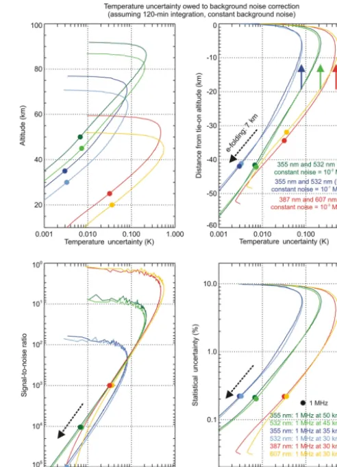
2 in Eq. (24) has almost no impact on the actual temperature uncertainty owing to detection noise. The temperature un-certainty owing to detection noise, as defined by Eq. (25), can be of any order of magnitude, depending on altitude and lidar performance and/or specification. Figure 1 shows this order of magnitude as a function of signal magnitude (left) and altitude (right) for a wide range of lidar specifications. A channel performance is defined here for a given sampling resolution as the altitude at which the signal count rate is 1 MHz. Using such generic representation allows the iden-tification of a family of curves, all of which have the same
e-folding rate with altitude and signal magnitude. This way, the actual order of magnitude of the temperature uncertainty can be inferred for any lidar system of specific performance. Not surprisingly, this uncertainty component’se-folding rate is approximately 14 km (black arrow on the right plot), which corresponds to the square root of the 7 kme-folding rate of air number density. The results in Fig. 1 are shown for a 120 min integration time and 50 Hz laser repetition rate. For an integration time that is 4 times shorter (30 min), all curves would shift to the right by a factor of 2. For a integration time that is 4 times longer (8 h), all curves would shift to the left by a factor of 2.
4.2 Uncertainty owing to saturation (pulse pile-up) correction
The uncertainty component owing to saturation correction depends on the hardware’s dead timeτ and its uncertainty
uτ, which are typically known from the technical specifica-tions provided by the hardware manufacturer (type B estima-tion). This uncertainty component is introduced where the signal is recorded in the data files (raw signalR). Using the subscript (SAT) for saturation, the saturation correction un-certainty propagated to the saturation and background-noise-corrected signalP is obtained by applying Eq. (2) to the sig-nal transformation Eq. (11):
uP (SAT)(k)= 2δz
cLP
2(k)u
τ. (29)
lidar-Figure 1. Temperature uncertainty owing to detection noise as a function of lidar signal magnitude (left) and altitude (right) for a variety of lidar performance configurations, specifically, two differ-ent signal strengths (1 MHz in the upper stratosphere and 1 MHz in the lower stratosphere), two different emission wavelengths (ul-traviolet and green), three different vertical samplings (15, 75, and 300 m), and two types of backscatter (Rayleigh and Raman). The solid circles indicate the location of the 1 MHz signal count rate for a specific channel.
derived relative densityN by applying Eq. (2) to the signal transformation Eq. (12):
uN (SAT)(k)=
N (k)
P (k)uP (SAT)(k). (30)
The saturation correction is applied to the lidar signals con-sistently at all altitudes. Its uncertainty is therefore propa-gated through Eq. (13), assuming full correlation between two consecutive altitudesz(k0) andz(k0+1). In these condi-tions, applying Eq. (2) to the signal transformation Eq. (15) yields
uN (SAT)(k0)=N (k 0)
2
u
N (SAT)(k0)
N (k0) +
uN (SAT)(k0+1)
N (k0+1)
. (31)
The saturation correction uncertainty then propagates to the sum S defined in Eq. (14), again assuming full correlation between altitude bins:
uS(SAT)(k)= kTOP−1
X
k0=k
g(k0)uN (SAT)(k0). (32)
Finally, the temperature uncertainty owing to saturation cor-rectionuT (SAT) is computed by applying Eq. (2) to the den-sity integration Eq. (13) with the same full correlation as-sumptions:
Figure 2.Temperature uncertainty owing to saturation correction as a function of lidar signal magnitude (left) and altitude (right) for a variety of lidar performance configurations (see Fig. 1 caption for details).
uT (SAT)(k)= 1
N (k) (33)
T (k)uN (SAT)(k)−Ta(kTOP)uN (SAT)(kTOP)− Maδz
Ra uS(SAT)(k)
.
Figure 2 shows the order of magnitude of this uncertainty component as a function of signal strength (left) and altitude (right) for two saturation correction cases, namely if the dead time is 20 ns (max. count rate of 50 MHz, dashed curves), and if the dead time is 4 ns (max count rate of 250 MHz, solid curves). As for detection noise uncertainty, the results are presented in generic form so that the actual order of mag-nitude of this uncertainty component can be easily estimated for lidar systems of any performance. Here, the same family of curves is obtained when the uncertainty is represented as a function of the ratio of the signal to the maximum counting rate (left plot).
4.3 Uncertainty owing to background noise extraction Background noise is typically subtracted from the total sig-nal by fitting the uppermost part of the lidar sigsig-nal with a constant, linear, or nonlinear function of altitude. An uncer-tainty component associated with the noise fitting procedure should be introduced. Here we consider the simple case of a linear fit, knowing that exactly the same approach can be used for other fitting functions. The linear fitting function to be estimated can be written as follows:
B(k)=b0+b1z(k). (34)
background noise, the background noise correction uncer-tainty can then be introduced by applying Eq. (2) to the signal transformation Eq. (11):
uP (BKG)(k)=
q
u2b0+u2b1z2(k)+2z(k)cov(b
0, b1). (35) The above expression can be expanded and/or modified based on the actual form of the fitting function, and tak-ing into account the fitttak-ing coefficients’ covariance matrix returned by the fitting routine. Just like the saturation cor-rection uncertainty, the uncertainty component owing to the background noise extraction can be propagated through the temperature retrieval, assuming full correlation in altitude. Applying Eq. (2) to the signal transformations Eqs. (12)–(15) therefore yields
uN (BKG)(k)=
N (k)
P (k)uP (BKG)(k) (36)
uN (BKG)(k0)= N (k 0)
2
uN (BKG)(k0) N (k0) +
uN (BKG)(k0+1) N (k0+1)
! (37)
uS(BKG)(k)= kTOP−1
X
k0=k
g(k0)uN (BKG)(k0) (38)
uT (BKG)(k)= 1
N (k) (39)
T (k)uN (BKG)(k)−Ta(kTOP)uN (BKG)(kTOP)− Maδz
Ra
uS(BKG)(k)
.
The order of magnitude of this uncertainty component de-pends on the magnitude of the background noise, and if signal-induced noise is present on the slope of this noise with respect to the signal slope. Figure 3 shows several ex-amples of constant background noise of varying magnitude. The temperature uncertainty is represented here as a function of altitude left), distance from the tie-on altitude (top-right), signal-to-noise ratio (bottom-left), and statistical un-certainty (bottom-right). The curves show a systematic pat-tern which consists of a rapid increase in the first 3–4 km below the tie-on altitude as density is integrated downward, followed by a decrease as we get further and further from the tie-on altitude. Thee-folding rate is 7 km for the entire fam-ily of curves, which reflects the main influence of the 1/N
term in Eq. (36). The temperature uncertainty maximum is larger when the magnitude of the noise is larger (as shown for the 387 and 607 nm Raman channels on Fig. 3).
4.4 Uncertainty owing to Rayleigh extinction cross sections
All lidar-derived relative density uncertainty components owing to the atmospheric extinction are computed by apply-ing Eqs. (2) to (12). The Rayleigh extinction cross sections
Figure 3.Temperature uncertainty owing to background noise cor-rection as a function of altitude left), distance from tie-on (top-right), signal-to-noise ratio (bottom left), and statistical uncertainty (bottom-right), for a variety of signal and noise strengths (see Fig. 1 caption for details).
4.4.1 Lidar-derived relative density uncertainty for Rayleigh backscatter channels
For Rayleigh backscatter channels, the received wavelength (λ2)is identical to the emitted wavelength (λ1), and the cross section uncertainty owing to random and systematic effects is introduced and propagated identically throughout the tem-perature retrieval. Using the subscript (σ M)0’ for molecular extinction cross section uncertainty component, and the suf-fixes R0 andS0 for random and systematic components re-spectively, the Rayleigh extinction cross section uncertainty owing to random and systematic effects can be propagated to the lidar-derived relative densityN by applying Eqs. (2) to (12):
uN (σ MX)(k)=2N (k)δz k
X
k0=0
Na(k0)uσ M_1X,
with X=R, S. (40)
4.4.2 Lidar-derived relative density uncertainty for Raman backscatter channels
For Raman backscatter channels (Strauch et al., 1971), the received and emitted wavelengths are different, and the cross section uncertainty owing to random and systematic effects is introduced and propagated differently. For the uncertainty component owing to random effect, applying Eqs. (2) to (11) yields
uN (σ MR)(k)=N (k)δz k
X
k0= 0
Na(k0)
q
u2σ M_1R+u2σ M_2R. (41)
For the uncertainty component owing to systematic effects, applying Eqs. (2) to (12) yields
uN (σ MS)(k)=N (k)δz k
X
k0=0
Na(k0) uσ M_1S+uσ M_2S. (42)
4.4.3 Propagation to temperature
For both Rayleigh and Raman backscatter, both random and systematic components of the lidar-derived relative density uncertainty owing to Rayleigh extinction cross sections are propagated to temperature similarly to the saturation and background uncertainty components (e.g., Eqs. 28–30):
uN (σ MX)(k0)=N (k 0)
2
uN (σ MX)(k0)
N (k0) +
uN (σ MX)(k0+1)
N (k0+1)
,
with X=R, S. uS(σ MX)(k)=
kTOP−1
X
k0=k
g(k0)uN (σ MX)(k0),
with X=R, S. (43)
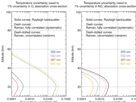
Figure 4.Temperature uncertainty owing to the Rayleigh cross sec-tion used in the molecular extincsec-tion correcsec-tion. The results are shown per 1 % in cross section uncertainty.
uT (σ MX)(k)= 1
N (k)
T (k)uN (σ MX)(k)−Ta(kTOP)uN (σ MX)(kTOP)
−Maδz Ra
uS(σ MX)(k)
, with X=R, S. (44)
The magnitude of the uncertainty owing to the Rayleigh cross sections is plotted in Fig. 4 for four different wavelengths and for components owing to both systematic and random effects. The results are shown for each 1 % cross section un-certainty; i.e., if the cross section is introduced in the lidar measurement model with a 5 % uncertainty, then the temper-ature uncertainty will be 5 times larger than shown in Fig. 4. Again for all curves, thee-folding rate is 7 km, which reflects the dominant influence of the term 1/N in Eq. (44).
4.5 Uncertainty owing to air number density
4.5.1 If air number density is the input quantity Here, it is assumed that the air density profile Na is made of fully correlated values in altitude. If air number density is not derived from air temperature and pressure, its uncer-taintyuNa is propagated to the lidar-derived relative density
by applying Eqs. (2) to (12) in a straightforward manner:
uN (Na)(k)=N (k)δz σM_1+σM_2
k
X
k0=0 uNa(k
0
). (45)
This component is then propagated to temperature using the same approach as for saturation and background noise cor-rection uncertainties.
4.5.2 If air temperature and pressure are the input quantities
When the ancillary number density is computed from an ancillary temperature Ta and pressure pa source (e.g., ra-diosonde measurements or meteorological models), the un-certaintiesuTa andupamust be introduced and the degree of
correlation between temperature and pressure must be esti-mated.
If temperature and pressure are measured or computed in-dependently, then the complete covariance matrix in the ver-tical dimension needs to be estimated. This is the most com-plex case to consider because of the interplay between the lack of correlation betweenTaandpa at any given altitude, and the high correlation between the temperature values at two consecutive altitudes, or between the pressure values at two consecutive altitudes. However, a good approximation consists of considering the propagation linear, i.e., first com-bining the uncertainties at one fixed level assuming no cor-relation, and then propagating the combined uncertainty as-suming full correlation between two consecutive altitudes. In this case, the lidar-derived relative density uncertainty owing to the ancillary air number density can be written as follows:
uN (Na)(k)=N (k)δz
k
X
k0=0
σM_1+σM_2Na(k0)
s
u2pa(k0) p2
a(k0)
+u
2 Ta(k
0)
T2 a(k0)
. (46)
If temperature and pressure are known to be fully correlated, then the lidar-derived relative density uncertainty owing to the ancillary air number density becomes
uN (Na)(k)= (47)
N (k)δz
k
X
k0=0
σM_1+σM_2
Na(k0)
upa(k0)
pa(k0)
−uTa(k 0)
Ta(k0)
.
4.5.3 Propagation to temperature
The lidar-derived number density uncertainty owing to an-cillary air number density is propagated to temperature by
Figure 5.Temperature uncertainty owing to the a priori use of ancil-lary air number density in the molecular extinction correction. The results are shown per 1 % ancillary number density uncertainty (left plot), and per 1 K and 0.1 hPa ancillary temperature and pressure uncertainty respectively (right plot).
applying Eq. (2) to Eqs. (13)–(15), assuming full correlation in altitude:
uN (N a)(k
0
)=N (k 0)
2
uN (Na)(k
0)
N (k0) +
uN (Na)(k
0+1) N (k0+1)
(48)
uS(Na)(k)=
kTOP−1
X
k0=k
g(k0)uN (N a)(k
0
) (49)
uT (Na)(k)=
1
N (k) (50)
T (k)uN (Na)(k)−Ta(kTOP)uN (Na)(kTOP)− Maδz
Ra
uS(Na)(k)
.
Figure 5 shows the magnitude of this uncertainty component, assuming either that the input quantity is the air number den-sity (left plot), or that the input quantities are temperature and pressure (right plot). In the first case, the results are shown for 1 % uncertainty in ancillary air number density. In the second case, the results are plotted for 1 K ancillary tempera-ture uncertainty (solid curves) and 0.1 hPa ancillary pressure uncertainty (dashed curves). The shape of the dashed curves do not show the normal 7 kme-folding rate because of the emerging very high pressure relative uncertainty associated with a fixed 0.1 hPa value. Thee-folding rate would be sim-ilar to the other curves if the ancillary pressure uncertainty were set to be constant in relative value rather than absolute. 4.6 Uncertainty owing to the ozone and NO2
absorption cross sections
(e.g., Brion et al., 1998; Daumont et al., 1992; Bogumil et al., 2003; Chehade et al., 2013; Gorshelev et al., 2014; Burkholder and Talukdar, 1994; Burrows et al., 1999; Van-daele et al., 1998). The random component of the cross sec-tion uncertainty is normally provided in these works. Occa-sionally, one or more components owing to systematic effects are also provided. For the ozone absorption cross section, a review and assessment of the available datasets is summa-rized in Sect. 3.5 and Appendix E of the ISSI team report (Leblanc et al., 2016a). Just like for Rayleigh extinction cross sections, these two types of component are not introduced and propagated identically in the lidar temperature measure-ment model. The formulation of their propagation is identical to that just presented for Rayleigh extinction cross sections (Eqs. 40–44), except that the air number density is replaced by the interfering gas number density, and the cross section uncertainty is now a function of temperature, i.e., altitude.
For Rayleigh backscatter channels,
uN (σigX)(k)=2N (k)δz k
X
k0=0 NO3(k
0
)uσig_1X(k0),
with ig=O3,NO2 and X=R, S. (51) For Raman backscatter channels,
uN (σigR)(k)=N (k)δz (52)
v u u t
k
X
k0=0
Nig2(k0)u2 σig_1R(k
0)+u2 σig_2R(k
0),
with ig=O3,NO2.
uN (σigS)(k)= (53)
N (k)δz
k
X
k0=0
Na(k0) uσig_1S(k0)+uσig_2S(k0), with ig=O3,NO2.
Their propagation to temperature can then be written as fol-lows:
uN (σigX)(k0)= (54)
N (k0)
2
u
N (σigX)(k0)
N (k0) +
uN (σigX)(k0+1)
N (k0+1)
,
with ig=O3,NO2 and X=R, S.
uS(σigX)(k)= kTOP−1
X
k0=k
g(k0)uN (σigX)(k0), (55) with ig=O3,NO2 and X=R, S.
uT (σigX)(k)= 1
N (k) (56)
T (k)uN (σigX)(k)−Ta(kTOP)uN (σigX)(kTOP)
−Maδz Ra
uS(σigX)(k)
ig=O3,NO2;X=R, S.
Figure 6.Temperature uncertainty owing to the cross sections used for the ozone and NO2absorption correction. The results are shown per 1 % in cross section uncertainty (left side: ozone, right side: NO2), and for components owing to both systematic and random
effects.
The magnitude of this uncertainty component owing to both systematic and random effects is shown in Fig. 6 for both Rayleigh and Raman backscatter cases and different wave-lengths. The contribution of ozone absorption (left plot) is larger in the visible (532 and 607 nm which are both in the Chappuis band) than in the ultraviolet spectrum (355 and 387 nm). Conversely, the contribution of NO2 absorp-tion (right plot) is larger in the ultraviolet than in the visible spectrum.
4.7 Uncertainty owing to ancillary ozone and NO2 number density profiles
The ozone and NO2absorption terms in Eq. (12) comprise the sum of ancillary ozone and NO2number densities taken at all altitudes from the ground to the altitude considered
z(k). Depending on the data source, these ancillary profiles may be mixing ratio or number density (Ahmad et al., 2007; Bauer et al., 2012; Bracher et al., 2005; Brohede et al., 2007). Assuming that all values within the same ancillary profile are fully correlated, uncertainty components owing to the ancil-lary ozone and NO2profiles can be propagated to tempera-ture similarly to the uncertainty component owing to air num-ber density (i.e., Eq. 45 and Eqs. 48–50):
uN (Nig)(k)=N (k) k
X
k0=0
σig_1(k0)+σig_2(k0)uN ig(k0),
with ig=O3,NO2, (57)
uN (Nig)(k0)=N (k 0
)
2
uN (Nig)(k0) N (k0) +
uN (Nig)(k0+1) N (k0+1)
Figure 7.Temperature uncertainty owing to the a priori use of an-cillary ozone number density (left) and NO2number density (right)
for the absorption correction. The results are shown per 1 % un-certainty (solid curves), and for 1 ppmv ozone unun-certainty (dashed curves, left) and 1 ppbv NO2uncertainty (dashed curves, right).
uS(Nig)(k)= kTOP−1
X
k0=k
g(k0)uN (Nig)(k0) (59)
uT (Nig)(k)= (60) 1
N (k)
T (k)uN (Nig)(k)−Ta(kTOP)uN (Nig)(kTOP)− Maδz
Ra
uS(Nig)(k)
.
Figure 7 shows the magnitude of this uncertainty com-ponent for both ozone (left) and NO2 (right), for both Rayleigh and Raman backscatter cases, and for different wavelength bands. The results are shown per 1 % ancillary ozone and NO2 uncertainty (solid curves), and per 1 ppmv ancillary ozone (respectively 1 ppbv ancillary NO2) tainty (dashed curves). Similarly to the temperature uncer-tainty owing to the absorption cross sections, the contribu-tion of ozone is larger in the visible than in the ultraviolet, and the contribution of NO2is larger in the ultraviolet than in the visible.
4.8 Uncertainty owing to the temperature tie-on at the top of the profile
Equation (12) shows that an ancillary temperature valueTa at altitude z(kTOP)is needed to initialize the profile at the top. Using the subscript (TIE) for tie-on, the ancillary tem-perature uncertaintyuTa(kTOP)is propagated to the retrieved
temperature profile by applying Eqs. (2) to (13):
uT (TIE)(k)=
N (kTOP)
N (k) uTa(kTOP). (61)
The magnitude of this uncertainty component is plotted in Fig. 8 for a 1 K tie-on ancillary temperature uncertainty and
Figure 8.Temperature uncertainty owing to a priori use of ancillary temperature to tie-on at the start of the density integration process. The results are shown per 1 K ancillary temperature uncertainty.
for several lidar performance cases. As expected, we obtain a family of curves with an approximatee-folding rate of 7 km due to the term 1/Nin Eq. (47).
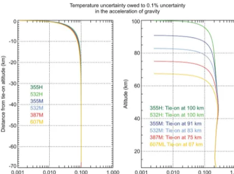
4.9 Uncertainty owing to the acceleration of gravity The acceleration of gravity is an input quantity introduced in Eq. (14). The constantsg0,g1, andg2relate to the Earth’s ge-ometry and to the geodetic latitude of the lidar site. If a value of the local ellipsoid height at the lidar siteh(0) is not known, we can approximate it to the site’s altitude above mean sea levelz(0). For all altitude-dependent and latitude-dependent formulations of the acceleration of gravity, the difference be-tweenh(0) andz(0) is by far the largest source of error in the computation of the acceleration of gravity. We therefore can define a new uncertainty componentuhassociated with the approximation ofh. The values ofhat neighboring alti-tudes are fully correlated, and their standard uncertainty can be deduced directly from Eq. (17):
uh k0=1
2 uh k 0
+uh k0+1. (62)
The height uncertainty is then propagated to temperature by applying Eq. (2) to Eqs. (13)–(16):
uT (g)(k)= (63)
1
N (k) Maδz
Ra
g0 kTOP−1
X
k0=k
N (k0) g1+2g2h(k0)
uh(k0).
Figure 9.Temperature uncertainty owing to 0.1 % uncertainty in the acceleration of gravity. Left: relative uncertainty (%) as a function of the distance from the tie-on altitude. Right: absolute uncertainty (K) as a function of altitude.
4.10 Uncertainty owing to the molecular mass of air The molecular mass of dry airMais introduced in Eq. (13). Its uncertaintyuMacan be propagated to temperature using uT (Ma)(k)=
δz Ra
S(k)
N (k)uMa. (64)
This component remains negligible below 90 km, and has a variation with altitude exactly similar to that shown for the acceleration of gravity. Figure 9 can therefore be used for the molecular mass of air without any change to it.
4.11 Propagation of uncertainty when vertically filtering (smoothing) the lidar signal or temperature profile
The smoothing procedure was introduced as an optional step in the measurement model. If present, it can be applied either to the lidar signal or to the retrieved temperature profile (see Eqs. 18–19).
4.11.1 Smoothing the lidar signal before the temperature profile is computed
From Eq. (17) and using the same notation, the uncertainty component owing to detection noise is propagated to the smoothed signal profile, assuming no correlation between the neighboring points:
usm(DET)(k)=sm(k)
v u u t
n
X
p=−n
c2 p(k)
u2s(DET)(k+p)
s2(k+p) . (65) For all other uncertainty components except temperature tie-on, acceleration of gravity, and the molecular mass of air,
full correlation is assumed between the neighboring points, and the uncertainty in the smoothed signal can be written as follows:
usm(X)(k)=sm(k) n
X
p=−n
cp(k)
us(X)(k+p)
s(k+p) , (66)
with X=SAT, BKG, σ MR, σ MS, Na, σigR, σigS, and
Nig.
The uncertainty components owing to temperature tie-on, acceleration of gravity, and the molecular mass of air are not included in the above expression because they are intro-duced later in the data processing. In this case, Eqs. (61)– (64) apply directly to the temperature profile retrieved from the smoothed lidar-derived number density.
4.11.2 Smoothing the retrieved temperature profile From Eq. (19) and using the same notation, the temperature uncertainty components owing to detection noise are propa-gated to the smoothed temperature profile, assuming no cor-relation between neighboring points:
uT m(DET)(k)=
v u u t
n
X
p=−n
c2
p(k)u2T (DET)(k+p). (67) For all other uncertainty components, full correlation is as-sumed between the two channels:
uT m(X)(k)= n
X
p=−n
cp(k)uT (X)(k+p), (68)
withX=SAT, BKG,σ MR,σ MS,Na,σigR,σigS,Nig,g,
TTOP, andMa.
4.12 Propagation of uncertainty when merging multiple channels together
The merging procedure was again introduced as an optional step in the measurement model. If present, it can be applied either to the lidar signals or temperature profiles.
4.12.1 Merging lidar signals before the temperature profile is computed
From Eq. (20) and using the same notation, the uncertainty components of the low and high channels owing to detection noise are propagated to the merged signal profile, assuming no correlation between the two channels:
usM(SDET)(k)=sM(k) (69)
s
w(k)usm(DET)(k, iL) sm(k, iL)
2
+
(1−w(k))usm(DET)(k, iH) sm(k, iH)
2
k1≤k≤k2 and 0≤w(k)≤1.
atmo-spheric extinction propagate to the merge density using
usM(X)(k)=sM(k) (70)
w(k)usm(X)(k, iL) sm(k, iL)
+(1−w(k))usm(X)(k, iH) sm(k, iH)
k1≤k≤k2 and 0≤w(k)≤1,
withX=σ MR,σ MS,Na,σigR,σigS, andNig.
For the uncertainty components of instrumental origin (namely, the saturation correction and background noise ex-traction), the degree of correlation between the channels hardware needs to be estimated before we can use a specific formulation for the propagation of the uncertainty compo-nents of instrumental origin. If the two channels use differ-ent hardware, they can be assumed to be independdiffer-ent, and the merged signal uncertainties owing to saturation correc-tion and background noise extraccorrec-tion can be written as fol-lows:
usM(SX)(k)=sM(k) (71)
s
w(k)usm(X)(k, iL) sm(k, iL)
2
+
(1−w(k))usm(X)(k, iH) sm(k, iH)
2
k1≤k≤k2 and 0≤w(k)≤1, withX=SAT, BKG.
If the two channels share the same hardware and if the sat-uration and background noise corrections have been applied consistently for both channels within the same data process-ing algorithm, the associated uncertainty components can be propagated to the combined profile, assuming full correla-tion:
usM(X)(k)=sM(k) (72)
w(k)usm(X)(k, iL) sm(k, iL)
+(1−w(k))usm(X)(k, iH) sm(k, iH)
k1≤k≤k2 and 0≤w(k)≤1, withX=SAT, BKG.
The uncertainty components owing to temperature tie-on, acceleration of gravity, and the molecular mass of air are not included in the above expressions because they are in-troduced later in the data processing. In this case, Eqs. (47)– (50) apply directly to the temperature profile retrieved from the merged lidar-derived number density.
4.12.2 Merging the temperature profiles retrieved for individual channels
From Eq. (21) and using the same notation, the temperature uncertainty components of the low and high channels owing to detection noise are propagated to the merged temperature
profile, assuming no correlation between the two channels:
uT M(DET)(k)= (73)
q
w(k)uT m(DET)(k, iL)2+ (1−w(k)) uT m(DET)(k, iH)2
k1≤k≤k2 and 0≤w(k)≤1.
For all uncertainty components that are not of instrumental origin, full correlation is assumed between the two channels:
uT M(X)(k)=w(k)uT m(X)(k, iL)+(1−w(k)) uT m(X)(k, iH)
k1≤k≤k2 and 0≤w(k)≤1, (74)
withX=σ MR,σ MS,Na,σigR,σigS,Nig,g,TTOP, and
Ma.
Just like in the case of merging the signals, for all uncer-tainty components of instrumental origin (namely, the satura-tion correcsatura-tion and background noise extracsatura-tion), the degree of correlation between the channels’ hardware needs to be es-timated. If the two channels use different hardware, they can be assumed to be independent, and the temperature uncer-tainties owing to saturation correction and background noise extraction can be written as follows:
uT M(X)(k)= (75)
q
w(k)uT m(X)(k, iL)
2
+ (1−w(k)) uT m(X)(k, iH)
2
k1≤k≤k2 and 0≤w(k)≤1, withX=SAT, BKG.
If the two channels share the same hardware and if the sat-uration and background noise corrections have been applied consistently for both channels within the same data process-ing algorithm, the associated uncertainty components can be propagated to the combined profile, assuming full correla-tion:
uT M(X)(k)=w(k)uT m(X)(k, iL)+(1−w(k)) uT m(X)(k, iH)
k1≤k≤k2 and 0≤w(k)≤1, (76)
withX=SAT, BKG.
4.13 Temperature combined standard uncertainty Now that all the independent uncertainty components consid-ered in our lidar temperature measurement model have been reviewed and propagated, we can combine them into a unique temperature combined standard uncertainty:
uT(k)=
v u u u u u u u u u u t
u2T (DET)(k)+u2T (SAT)(k)+u2T (BKG)(k) +u2T (TTOP)(k)+u2T (σ MR)(k)
+u2T (σ MRS)(k)+u2T (N
a)(k)+u
2 T (g)(k)
+u2T (M
a)(k)+u
2
T (σO3R)(k)+u
2
T (σO3S)(k) +u2T (NO
3)(k)+u
2
T (σNO2R)(k) +u2T (σNO
2S)(k)+u
2
T (NNO2)(k).