www.the-cryosphere.net/8/867/2014/ doi:10.5194/tc-8-867-2014
© Author(s) 2014. CC Attribution 3.0 License.
The Cryosphere
Transition of flow regime along a marine-terminating outlet glacier
in East Antarctica
D. Callens1, K. Matsuoka2, D. Steinhage3, B. Smith4, E. Witrant5,1, and F. Pattyn1
1Laboratoire de Glaciologie, Université Libre de Bruxelles, Brussels, Belgium 2Norwegian Polar Institute, Tromsø, Norway
3Alfred-Wegener-Institut Helmholtz-Zentrum für Polar- und Meeresforschung, Bremerhaven, Germany 4Applied Physics Laboratory, University of Washington, Seattle, WA, USA
5GIPSA-lab, Université Joseph Fourrier, Grenoble, France
Correspondence to: D. Callens (dcallens@ulb.ac.be)
Received: 10 September 2013 – Published in The Cryosphere Discuss.: 7 October 2013 Revised: 21 March 2014 – Accepted: 25 March 2014 – Published: 13 May 2014
Abstract. We present results of a multi-methodological ap-proach to characterize the flow regime of West Ragnhild Glacier, the widest glacier in Dronning Maud Land, Antarc-tica. A new airborne radar survey points to substantially thicker ice (>2000 m) than previously thought. With a dis-charge estimate of 13–14 Gt yr−1, West Ragnhild Glacier thus becomes of the three major outlet glaciers in Dronning Maud Land. Its bed topography is distinct between the up-stream and downup-stream section: in the downup-stream section (<65 km upstream of the grounding line), the glacier over-lies a wide and flat basin well below the sea level, while the upstream region is more mountainous. Spectral analy-sis of the bed topography also reveals this clear contrast and suggests that the downstream area is sediment covered. Furthermore, bed-returned power varies by 30 dB within 20 km near the bed flatness transition, suggesting that the water content at bed/ice interface increases over a short dis-tance downstream, hence pointing to water-rich sediment. Ice flow speed observed in the downstream part of the glacier (∼250 m yr−1) can only be explained through very low basal friction, leading to a substantial amount of basal sliding in the downstream 65 km of the glacier. All the above lines of evi-dence (sediment bed, wetness and basal motion) and the rel-atively flat grounding zone give the potential for West Ragn-hild Glacier to be more sensitive to external forcing com-pared to other major outlet glaciers in this region, which are more stable due to their bed geometry (e.g. Shirase Glacier).
1 Introduction
The overall mass balance of the Antarctic ice sheet is dom-inated by a significant mass deficit in West Antarctica (Rig-not et al., 2008; Pritchard et al., 2012). This is primarily due to thinning and acceleration of glaciers (e.g. Pine Island Glacier; Joughin et al., 2003) mainly driven by the loss of buttressing from ice shelves (Schoof, 2010). Concurrently, the trend in East Antarctica is weaker. The East Antarctic ice sheet (EAIS) is only losing mass slightly, as increased surface accumulation compensates mass loss through outlet glaciers (Shepherd et al., 2012). While Miles et al. (2013) observe a link between front migration and climate forcing, a significant widespread thinning trend along the pacific coast of the EAIS remains lacking.
Although East Antarctica is mainly continental, limited observations in Dronning Maud Land (DML), show that the ice sheet seaward of the inland mountains lies on a bed well below sea level (BEDMAP2; Fretwell et al., 2013) and most of the ice from the polar plateau is discharged through nu-merous glaciers in between coastal mountain ranges. The ice-dynamical consequences of such settings have yet to be ex-plored. In this paper we investigate the marine boundary of such a glacier system draining the EAIS in DML.
75°S 70°S
10°W
45°E (a)
BM SRM
Polar Stereographic Easting (km)
Polar Stereographic Northing (km)
800 850 900 950 1000 1050 1100 1150 1200 1600
1650 1700 1750 1800 1850 1900 1950 2000
Suface Speed (m/a)
0 50 100 150 200 250 300
500 m.a.s.l
1000
1500
2000 (b)
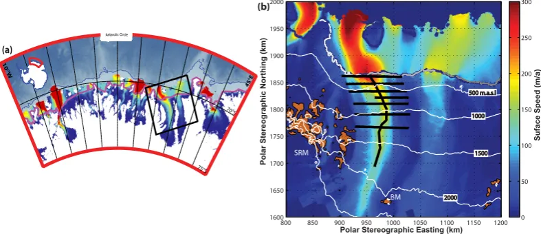
Fig. 1. Overview map of West Ragnhild Glacier, Dronning Maud Land, East Antarctica. (a) Dronning Maud Land. Ice flow speed is shown on the same scale as for panel (b) (but white when<15 m yr−1; Rignot et al., 2011a). The grounding line is shown in purple (Bindschadler et al., 2011). Rock outcrops are shown in brown (SCAR, 2012). The square shows the 400 km×400 km area covered by the map on panel (b). The inset shows the coverage of panel (a). (b) West Ragnhild Glacier. Background colour shows the surface flow speed derived from satellite interferometry and speckle tracking. Contours show surface elevations at 500 m interval (Bamber et al., 2009). From west to east, the grounding line is defined on the basis of a pair of PALSAR images taken in 2007 (light grey) and two pairs of RADARSAT (middle grey and dark grey) taken in 2000 (Rignot et al., 2011b). Black lines are the longitudinal and transverse radar profiles. Rock outcrops as in (a). SRM and BM stand for Sør Rondane Mountains and Belgica Mountains, respectively.
the ice shelf locally grounded. Potential unpinning of these ice shelves would inevitably lead to ice shelf speed up, which makes them sensitive to marine forcing.
Of all glaciers in DML, West Ragnhild Glacier is the widest (≈90 km) and longest. Its ice flow speed is al-ready 100 m yr−1250 km upstream from the grounding line (Fig. 1b). Based on the ice thickness data presented in this paper, we estimate the grounding line mass flux to be 13– 14 Gt yr−1, which constitutes roughly 10 % of the total
dis-charge from DML (Rignot et al., 2008). This is of the same order of magnitude as Shirase Glacier (13.8±1.6 Gt yr−1;
Pattyn and Derauw, 2002) and Jutulstraumen (14.2 Gt yr−1; Høydal, 1996), the other two major outlet glaciers in the DML region.
The stability of West Ragnhild Glacier is most likely gov-erned by the dynamics of its ice shelf which is dominated by two important ice rises and several pinning points. While rapid changes at the marine boundary have not yet been ob-served, Rignot et al. (2013) point to an exceedance of basal melt (underneath the ice shelf and at the grounding line) over calving for several ice shelves in DML (including Roi Baudouin Ice Shelf, downstream of West Ragnhild Glacier). Melting at the grounding line 50 km west from West Ragn-hild Glacier has been reported in Pattyn et al. (2012), but its magnitude is of the orders of tens of centimetres per year.
To understand what makes West Ragnhild Glacier one of the three most significant mass outputs in DML, we investi-gate its basal conditions using satellite remote sensing, air-borne radar and ice sheet modelling. First, radar analysis reveals the geometry of the bed. Second, we characterize
the roughness of the bed and its reflectivity through spec-tral and bed-returned power analyses, which inform us of the nature of the bed as well as of the water content. Fi-nally, we estimate the basal friction through inverse mod-elling to reconstruct basal motion. We subsequently discuss the consequences of a marine-terminating East Antarctic out-let glacier, characterized by a wet sediment and dominated by basal motion/sliding.
2 Data acquisition
Ice flow surface velocities are generated based on RADARSAT data acquired during the austral spring of 2000. These velocities combine phase and speckle tracking offsets, using methods that minimize the error of the final combined product (Joughin, 2002). The resolution of the velocity data is 500 m×500 m, covering the main trunk of West Ragnhild Glacier and its vicinity (Fig. 1b).
0 20 40 60 80 100 120 140 160 180 −1200
−600 0 600 1200
Distance from the grounding line (km)
El
e
v
a
ti
o
n
(m
.a
.s
.l
.)
−60 −40 −20 0 20 40 60
500 m
I
II
III
IV
V
VI
VII
Easting from the centre flowline (km) Ice Thickness (m)
600 800 1000 1200 1400 1600 1800 2000 2200
a
b
Downstream region Upstream region
I II III IV V VI VII
20
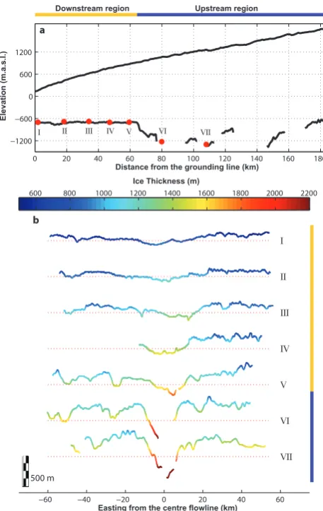
Fig. 2. Radar data. (a) Ice and bed topography along the cen-tral flowline. The red circles are the locations of the cross pro-files. (b) Bed topography (ordinate) and ice thickness (colour) measured across the flow. The red dotted lines show the isodepth of 600 m b.s.l., the approximate elevation of the flat basin mea-sured along the centre flowline (a) and the reference for each pro-file.Transverse profiles are numbered from I to VII on both panels. The yellow and blue line illustrates our understanding of the down-stream and updown-stream region.
(Fig. 2). Most sections lacking a bed echo are shorter than
∼10 km (the maximum data gap is 20 km). Adjacent regions to these data gaps slope down steeply toward the data gaps. Therefore, the data gaps probably correspond to a deep bed and thick ice, causing an increased radar signal attenuation, and hence loss of signal.
Ice thickness was derived using a constant radio wave propagation speed of 168 m µs−1. Surface elevation was ob-tained by laser altimetry from the aircraft, and bed elevation was subsequently derived by subtracting the ice thickness from the surface elevation. We applied the geoid height of 20 m above the EGM96 ellipsoid (Rapp, 1997) to derive the surface and bed elevations relative to sea level.
3 Mapping the subglacial topography
Compared to older data sets of Antarctic bedrock topography (e.g. BEDMAP; Lythe et al., 2001), our new radar survey re-veals a significantly different picture1. The survey highlights a marked contrast in bed topography (Fig. 2). Between the Sør Rondane and Belgica Mountains, ice flows in a deeply in-cised valley,∼20 km wide, lying∼1000 m below sea level at the two uppermost transverse profiles (Fig. 2b). The bed topography is rather variable here, fluctuating between 1200 and 800 m b.s.l. Further downstream, bedrock elevation in-creases rapidly (more than 500 m within 10 km distance) up to a flat subglacial lowland lying around 600 m b.s.l. This can be observed on both the longitudinal (Fig. 2a) and cross pro-files (Fig. 2b). The elevation of this lowland varies less than 50 m locally, so the lowland is much flatter than the landward valley between Sør Rondane and Belgica Mountains. The amplitude of the local elevation variations increases sharply between cross profiles 4 and 5 as we reach the piedmont of the Sør Rondane Mountains. This is also the zone where we find the onset of the subglacial valley, described earlier.
4 Spectral analysis of bed topography
4.1 Bed roughness index
One way to quantitatively characterize the above-described bed conditions is to calculate bed roughness. The bed rough-ness index RI is obtained by applying a fast Fourier trans-form (FFT) to the bed elevation within a moving window (Taylor et al., 2004):
RI=
fmax
Z
fmin
|X[f]|2
NT1x
df , (1)
wherefmin=1/(NT1x),fmax=1/(21x),NT=2n is the
number of data points in the window, 1x is the sampling interval (100 m in our case) and where
X[f] =
NT
X
d=1
x(d)e
2π i
NT(d−1)(f−1). (2)
Equation (2) is the definition of the FFT for a datasetx(d) with indexd in the range 1≤d≤NT, andX[f]is the same
data set in the frequency domain with indexf in the range fmin≤f ≤fmax. In other words, the bed roughness index RI
is the integral of the resultant power spectrum within each of the moving windows.
We first resample the radar-derived bed topography (80±20 m intervals) with a fixed (100 m) interval. We then detrend the measured bed elevation in each moving window,
1The data collected for this paper are incorporated in the recently
which is required to be able to perform an FFT. The method is applied within a 2ndata point window. Several authors rec-ommend n≥5 (Taylor et al., 2004; Bingham and Siegert, 2009; Rippin et al., 2011). By usingn=6 we are able to analyse roughness over wavelengths ranging from 200 up to 6400 m.
4.2 Results
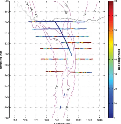
The longitudinal bed profile (Fig. 2) reveals two distinct ar-eas: a flat area (between the grounding line and 65 km up-stream) and an intersected subglacial relief typical of sub-glacial mountain ranges. The transition between them oc-curs within 10 km. The bed roughness index RI is capable of quantifying this difference (Figs. 3 and 4a). While the two regions are still quite distinct, the transition of roughness from one to the other is more gradual than expected from vi-sual interpretation. For the downstream cross profiles (I–III), the bed roughness is approximately constant, pointing to a wide and relatively smooth lowland. Following the analysis of Bingham and Siegert (2009), the flat and smooth area in the downstream section of the West Ragnhild Glacier may therefore very well be overlain by marine sediment. Accord-ing to the further upstream profiles (IV–V), the bed is rougher away from the current glacier flowline (longitudinal radar profile). The low roughness area is therefore restricted to the zones of fast ice flow. Once outside this section, bed rough-ness indices increase, pointing to a rougher surface (VI–VII).
5 Analysis of bed-returned power
5.1 Analytical setup
To further examine the spatial distribution of basal condi-tions, we analyse the radar power returned from the bed, hereafter called BRP. The geometrically corrected BRP, BRPc, can be seen as a proxy for bed reflectivity if englacial effects do not vary along the radar profile (Matsuoka, 2011). The BRPcis affected by both englacial attenuationLand bed reflectivityR. In the decibel scale,[x]dB=10 log10(x), this relationship can be written as
[BRPc]dB= [BRP]dB+10 log10
h+H
n
2
,
' [R]dB− [L]dB. (3)
The geometrically corrected bed-returned power BRPc can be calculated based on the measured BRP returned from the bed and a geometric factor defined by(h+H /n)2. Here,his the height of the aircraft above the glacier surface,H is the ice thickness (distance between the surface and the bed of the ice mass), andnis the refraction index of the ice (∼1.8; Matsuoka et al., 2012). The BRPcis then normalized to the mean of the observed values.
880 900 920 940 960 980 1000 1020 1040
1680 1700 1720 1740 1760 1780 1800 1820 1840 1860 1880 1900
Easting (km)
Northing (km
)
100 100
150
150
200 150 100
200
150
100 100
Bed roughness
0 10 20 30 40 50 60 70 80
Fig. 3. Bed roughness analysis. Bed roughness index of the basal to-pography (colour) calculated for wavelengths ranging from 200 to 6400 m. The grounding line is the same as in Fig. 1b. Short legs of absent bed echoes result in long gaps in the estimated bed roughness indices due the window-based calculation of the bed roughness in-dex. Larger RI corresponds to rougher bed. Contour lines represent surface speed (m a−1).
One has to note that effects of temporal changes in the instrumental characteristics and of ice crystal alignments are ignored in Eq. (3). Englacial attenuation has contribu-tions from pure ice and chemical constituents included in the glacier ice, both of which depend exponentially on ice tem-perature.
We estimate attenuationLusing Eqs. (4)–(6) listed below (Matsuoka et al., 2012). The depth-averaged attenuation rate
hNiis derived from the depth profile of the attenuation rate N (z), i.e.,
[L]dB=
H Z
0
N (z)dz . (4)
The attenuation profileN (z)is proportional to local ice con-ductivityσ:
N (z)=1000(10 log10e)
c ε0 √
ε σ (z)≈0.914σ (z) , (5)
wherecis the wave velocity in vacuum,ε0is the
0 10 20 30 40
Bed Roughness
0 20 40 60 80 100 120 140 160 180 200
50 60 70 80
Bed reflectivity (dB)
Distance from the grounding line (km) −20
0 20
BRP
c(dB)
40 50 60 70 80
Total attenuation (dB)
(a)
(b)
(c)
(d)
Fig. 4. Subglacial conditions along the central flowline. (a) Bed roughness index RI; (b) geometrically corrected bed-returned power BRPc; (c) englacial attenuationL; (d) bed reflectivityR.
an Arrhenius-type relationship.
σ=σ0exp
−E0
k
1
T (z)− 1 Tr
, (6)
whereσ0=15.4 µS m−1 is the pure-ice conductivity at the
reference temperatureTr=251 K, T (z)is the vertical
pro-file of temperature,E0=0.33 eV is the activation energy and
k=8.617×10⁻⁵eV K−1 is the Boltzmann constant (Mat-suoka et al., 2012).
Englacial temperatures T (z) for the attenuation model (Eq. 6) are calculated using a two-dimensional thermome-chanical higher-order model (Pattyn, 2002, 2003). Details of this approach are given in Matsuoka et al. (2012). We use a geothermal heat flux of 42 mW m−2as lower bound-ary condition. However, as shown in Matsuoka et al. (2012), the exact choice of geothermal heat flux will not affect the modelled englacial attenuation since the bed in the surveyed domain is predicted to be at the pressure melting point ev-erywhere even with a flux as low as 42 mW m−2. Once the bed reaches pressure melting point, additional geother-mal and shear heating have virtually no impact on ice tem-perature, hence on englacial attenuation (Matsuoka, 2011). Therefore, the estimated along-flow patterns of the attenua-tion and bed reflectivity are robust regardless of the uncer-tainties in geothermal heat flux. Figure 4c shows[L]along the longitudinal profile.
Although the chemical contribution to attenuation can nearly equal the pure-ice contribution near the coast (Mat-suoka et al., 2012), the lack of observation forces us to ig-nore its contribution and to use only the pure-ice contribu-tion to estimate englacial attenuacontribu-tion. Furthermore, MacGre-gor et al. (2007) and Matsuoka et al. (2012) showed that the relative importance of impurities contribution decreases as temperature increases. The modelling reveals a mean attenu-ation rate from pure ice between 20.2 and 23.1 dB km−1. For this range of value, Matsuoka et al. (2012) determine that chemical contribution is less than the fifth of the pure ice contribution.
5.2 Results
In the upstream valley, BRPc remains relatively low (−20 dB) and varies little (several dB) except at two sites where BRPcshows anomalous features (90 km and 170 km upstream from the grounding line; Fig. 4b). Further down-stream, BRPcincreases by∼50 dB within 20 km, over which the ice thins only by∼200 m (Fig. 2).
To clarify contributions of the bed reflectivity on BRPc, we estimate the englacial attenuation using the predicted temperature (Fig. 4c). Attenuation decreases∼20 dB within 10 km at 65 km upstream from the grounding line due to a decrease in ice thickness. Further downstream, attenuation gradually decreases by 20 dB over 50 km, which is probably more related to the changes in ice thickness than to changes in depth-averaged attenuation ratehNi. To retrieve the ac-tual bed reflectivity, we estimated bed reflectivity from BRPc and englacial attenuation using Eq. (3). The corresponding estimated bed reflectivity rapidly increases, approaching the grounding line at 40–50 km, from where it varies little within the last ∼30 km (Fig. 4d). The high bed reflectivity in the zone immediately upstream of the grounding line may even-tually point to wet bed conditions. This high bed reflectivity is not directly related to the smoother bed interface because RI is calculated for the wavelengths longer than 200 m but the reflectivity is affected by the bed smoothness in the scale of several wavelengths of the radio wave (5 m for this study). In the next section, we will investigate whether wet basal con-ditions are likely or not.
6 Ice flow modelling
6.1 Model setup
0 50 100 150 200 250 300 350 400
Speed (m/a)
Measured A B C D E
0 50 100 150 200 250 300
102
103
104
105
106
107
108
Basal friction parameter
Distance from the grounding line (km)
0 50 100 150 200 250 300 350 400
Surface speed (m/a)
(a)
(b)
(c)
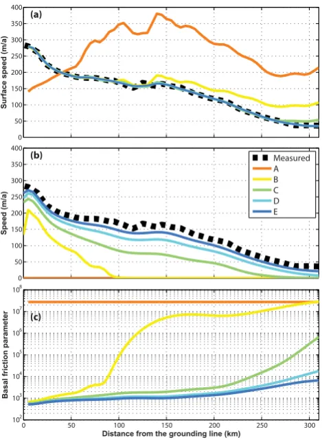
Fig. 5. (A) Observed surface flow speed (dashed black line) and optimized surface flow speed profiles along the central flowline of West Ragnhild Glacier; (B) Basal ice flow speed according to the optimization and compared to the satellite-observed surface flow speed (as in panel A); (C) Basal frictionβ2along the flowline.
order to minimize the misfit between modelled and observed velocities (MacAyeal, 1992, 1993; Arthern et al., 2010).
As a forward model we apply a simple ice flow model to calculate the ice flow field along the central flowline of West-ern Ragnhild Glacier, based on the shallow-ice approxima-tion (SIA). In the vertically integrated case, the SIA surface velocity (u(s)) is then given by
u(s)=u(b)+ 2A
n+1H|τd|
n−1τ
d, (7)
whereτd= −ρgH∂x∂s is the driving stress, andu(b)=β−2τd
is the basal velocity according to a viscous sliding law (Pat-tyn et al., 2008). Other parameters in Eq. (7) areAandn=3, the vertically integrated temperature-dependent flow param-eter and the exponent in Glen’s flow law, respectively;β is the basal friction,ρis the ice density,gis the gravitational acceleration,H is the ice thickness, andsis the surface el-evation. For a flowline stretching from the ice divide (Dome Fuji) to the grounding line, boundary conditions for Eq. (7) are a zero upstream velocity and a fixed surface velocity at
the edge of our profile ofu=300 m yr−1, according to
ob-servations.
Since an SIA model does not take into account longitu-dinal stress gradients, spurious high-frequency variability in the velocity field is to be expected when the surface of the ice sheet is not supposed to relax to the imposed stress field. Es-pecially small variations in surface slope may lead to a large variability in velocity, due to its dependence on the power ofn. To prevent this, surface gradients are calculated over a distance of several ice thicknesses (Kamb and Echelmeyer, 1986; Rabus and Echelmeyer, 1997).
The main unknown in Eq. (7) is the basal velocity field, which is initialized with a high value of basal friction (β2=
107), corresponding to conditions of ice frozen to the bed. We then invoke an optimization procedure to determine the spatial distribution ofβ2so that the modelled surface veloc-ity (ums ) matches the observed one (uos). This is formulated as a least-squares problem for which we seekβ2that minimizes the following objective function:
J (βˆ2)=
no
X
i=1
kuos(i)−ums(βˆ2, i)k2. (8)
The minimization problem is solved in a vector-valued ap-proach. The vector containing the squared errors of the basal velocity mismatch is provided to the algorithm that calculates the flow field according to Eq. (7). The error vector is used to compute a preconditioned conjugate gradient (computed numerically using small variations in β2 along the flow-line). The subspace trust region method based on the interior-reflective Newton method (trust-region-interior-reflective algorithm) described by Coleman and Li (1994, 1996) then determines the modifiedβ2-profile for the next iteration. The iterations stop when the change inJ (βˆ2)is below an arbitrarily small threshold.
We add two constraints toβ2. It has to be positive and, as we expect the basal friction pattern to be continuous in space (i.e.u(b) is continuously differentiable), the spatial pattern is expressed in terms of summations of Legendre polynomi-als. Such polynomials have the interesting property that they form an orthogonal basis and lead to a better conditioning of the nonlinear optimization problem, thus necessitating fewer iterations to converge to the optimal solution. We use these polynomials to describe the spatial distribution ofβ2along the flowline. We use polynomials up to degree 35. At this stage, we reach convergence, which means that increasing the polynomial degree does not reduce the error function any further.
linearly interpolated; the length of such gaps is typically less than several ice thicknesses, so that the large-scale flow fields are hardly affected by this choice. Longer gaps (>10 km) were interpolated in the same way. Bed topography uncer-tainties associated with the longer data gaps introduces flow speed uncertainties in the most upstream area and are suffi-ciently far away from our region of interest.
6.2 Results
To correct for the unknown deformational velocity, we per-formed the optimization procedure for different values of the vertically integrated flow parameterA. Each of the val-ues corresponds to mean ice temperatures of −2, −4,−5,
−10 and −15◦C (Cuffey and Paterson, 2010). Amongst the five different flow parameters depicted in Fig. 5, case A corresponds to the warmest (softest) ice (−2◦C), and
pre-dicts higher ice flow speeds due to ice deformation along the whole flowline compared to the observed ones. For this value, the optimization procedure fails, as the model cannot allow “negative” basal velocities. Not only is the ice too soft (hence flows too fast), the pattern of the deformational veloc-ity does not match the observed velocveloc-ity profile.
Cases B to E reveal a good match of the modelled veloci-ties with the observed ones. For each decrement in ice tem-perature, the ice gets stiffer and the amount of basal sliding along the profile becomes more important. Therefore, cases D and E correspond to much colder (stiffer) ice (−10 and
−15◦C, respectively) and predict deformational velocities that are too small, so that basal sliding takes up the major-ity of the velocmajor-ity along the profile.
The corresponding pattern ofβ2is, with the exception of case A, very similar for all simulations: it reveals a relatively high friction inland and a low friction in the area 100 km up-stream from the grounding line. Over the upup-stream section of the longitudinal profile, ice motion is essentially governed by internal deformation. All experiments show that basal motion is dominant only in the downstream region.
7 Discussion and conclusions
Prior to our study, only two glaciers were considered as im-portant contributors to the discharge of ice from DML, i.e. Jutulstraumen and Shirase Glacier, and both have been the subject of more interest in the past (e.g. Høydal, 1996; Pat-tyn and Derauw, 2002). Despite their fast flow (the grounding line velocity of Shirase Glacier is>2000 m yr−1), they each
discharge approximately 10 % of the total snow accumula-tion of this part of the ice sheet (Rignot et al., 2008). Both glaciers are topographically constrained and characterized by a highly convergent flow regime. They also terminate in a rel-atively narrow trunk. From an ice-dynamical viewpoint, Shi-rase Glacier is a relatively stable feature, as its grounding line cannot retreat over a distance larger than 5 to 10 km, since the
bedrock rapidly rises above sea level from the present posi-tion of the grounding line (Pattyn, 1996, 2000; Pattyn and Derauw, 2002). Such conditions make an outlet glacier less prone to dynamic grounding line retreat and significant mass loss due to dynamic changes in the ice shelf.
Taking into consideration West Ragnhild Glacier defi-nitely changes the discharge picture in DML. Indeed, based on the thickness data across the grounding line in conjunc-tion with satellite-observed ice flow velocities, its discharge (13–14 Gt yr−1) is comparable to the discharge of Jutulstrau-men and Shirase Glacier. Nonetheless, the ice flow velocities of West Ragnhild Glacier are relatively low. Ice flow speed is >100 m yr−1 at 100 km upstream of the grounding line and up to 250 m yr−1at the grounding line (Fig. 1). The rea-son for such low values is ice shelf buttressing by two major ice rises within the Roi Baudouin Ice Shelf, slowing down the flow upstream. While according to Rignot et al. (2008), the area seemed to be in balance, a significant imbalance is currently observed in the grounding zone of West Ragnhild Glacier and along the grounding line of the Roi Baudouin Ice Shelf (Rignot et al., 2013), which is in line with direct observations (Pattyn et al., 2012).
Despite present-day stable conditions, the analysis pre-sented in this paper clearly demonstrates that West Ragn-hild Glacier (i) is an important outlet glacier, (ii) is marine terminating with a grounding line 600–700 m b.s.l., and (iii) has a downstream section that is smooth, sediment covered and water saturated in the downstream area. Beside data evi-dence, inverse modelling allows the conclusion that decreas-ing basal friction leads to an increasdecreas-ing basal velocity to-wards the grounding line. Using two different kinds of evi-dence, we demonstrate that the bed/ice interface plays a dom-inant role in the acceleration of West Ragnhild Glacier to-ward the grounding line.
Acknowledgements. The radar survey was conducted by the Alfred Wegener Institute with further logistical support from the Princess Elisabeth Station (Belgian Antarctic Research Expedition, BELARE), and funded by the European Facilities for Airborne Research (EUFAR). D. Callens is funded through a FNRS-FRIA fellowship (Fonds de la Recherche Scientifique) and received an Yggdrasil mobility grant (Research Council of Norway). This work is in part supported by the Centre for Ice, Climate and Ecosystems (ICE) at the Norwegian Polar Institute.
Edited by: C. R. Stokes
References
Arthern, R. J. and Gudmundsson, G. H.: Initialisation of Ice-Sheet Forecasts viewed as an Inverse Robin Problem, J. Glaciol., 56, 527–533, 2010.
Bamber, J. L., Gomez-Dans, J. L., and Griggs, J. A.: A new 1 km digital elevation model of the Antarctic derived from combined satellite radar and laser data – Part 1: Data and methods, The Cryosphere, 3, 101–111, doi:10.5194/tc-3-101-2009, 2009. Bindschadler, R. A., Choi, H., and ASAID Collaborators:
High-Resolution Image-derived Grounding and Hydrostatic Lines for the Antarctic Ice Sheet, Digital media, National Snow and Ice Data Center, Boulder, Colorado, USA, 2011.
Bingham, R. G. and Siegert, M. J.: Quantifying subglacial bed roughness in Antarctica: implications for ice-sheet dynamics and history, Quaternary Sci. Rev., 28, 223–236, 2009.
Coleman, T. and Li, Y.: On the Convergence of Reflective New-ton Methods for Large-Scale Nonlinear Minimization Subject to Bounds, Math. Program., 67, 189–224, 1994.
Coleman, T. and Li, Y.: An Interior, Trust Region Approach for Nonlinear Minimization Subject to Bounds, SIAM J. Optimiz., 6, 418–445, 1996.
Cuffey, K. and Paterson, W. S. B.: The Physics of Glaciers, 4th Edn., Elsevier, New York, 2010.
Fretwell, P., Pritchard, H. D., Vaughan, D. G., Bamber, J. L., Bar-rand, N. E., Bell, R., Bianchi, C., Bingham, R. G., Blankenship, D. D., Casassa, G., Catania, G., Callens, D., Conway, H., Cook, A. J., Corr, H. F. J., Damaske, D., Damm, V., Ferraccioli, F., Fors-berg, R., Fujita, S., Gim, Y., Gogineni, P., Griggs, J. A., Hind-marsh, R. C. A., Holmlund, P., Holt, J. W., Jacobel, R. W., Jenk-ins, A., Jokat, W., Jordan, T., King, E. C., Kohler, J., Krabill, W., Riger-Kusk, M., Langley, K. A., Leitchenkov, G., Leuschen, C., Luyendyk, B. P., Matsuoka, K., Mouginot, J., Nitsche, F. O., Nogi, Y., Nost, O. A., Popov, S. V., Rignot, E., Rippin, D. M., Rivera, A., Roberts, J., Ross, N., Siegert, M. J., Smith, A. M., Steinhage, D., Studinger, M., Sun, B., Tinto, B. K., Welch, B. C., Wilson, D., Young, D. A., Xiangbin, C., and Zirizzotti, A.: Bedmap2: improved ice bed, surface and thickness datasets for Antarctica, The Cryosphere, 7, 375–393, doi:10.5194/tc-7-375-2013, 2013.
Høydal, Ø. A.: A force-balance study of ice flow and basal con-ditions of Jutulstraumen, Antarctica, J. Glaciol., 42, 413–425, 1996.
Joughin, I.: Ice-sheet velocity mapping: a combined interferomet-ric and speckle-tracking approach, Ann. Glaciol., 34, 195–201, 2002.
Joughin, I., Rignot, E., Rosanova, C. E., Lucchitta, B. K., and Bohlander, J.: Timing of Recent Accelerations of Pine Island Glacier, Antarctica, Geophys. Res. Lett., 30, 1706, doi:10.1029/2003GL017609, 2003.
Kamb, B. and Echelmeyer, K. A.: Stress-gradient Coupling in Glacier Flow: 1. Longitudinal Averaging of the Influence of Ice Thickness and Surface Slope, J. Glaciol., 32, 267–298, 1986. Lythe, M. B., Vaughan, D. G., and BEDMAP consortium:
BEDMAP: a new ice thickness and subglacial topographic model of Antarctica, J. Geophys. Res., 106, 11335–11351, 2001. MacAyeal, D. R.: The basal stress distribution of Ice Stream E,
Antarctica, inferred by control methods, J. Geophys. Res., 97, 595–603, 1992.
MacAyeal, D. R.: A Tutorial on the Use of Control Methods in Ice-Sheet Modeling, J. Glaciol., 39, 91–98, 1993.
MacGregor, J. A., Winebrenner, D. P., Conway, H.,Matsuoka, K., Mayewski, P. A., and Clow, G. D.: Modeling englacial radar attenuation at Siple Dome, West Antarctica, using ice chem-istry and temperature data, J. Geophys. Res., 112, F03008, doi:10.1029/2006JF000717, 2007.
Matsuoka, K.: Pitfalls in radar diagnosis of ice-sheet bed conditions: Lessons from englacial attenuation models, Geophys. Res. Lett., 38, L05505, doi:10.1029/2010GL046205, 2011.
Matsuoka, K., MacGregor, J. A., and Pattyn, F.: Predicting radar attenuation within the Antarctic ice sheet, Earth Planet. Sc. Lett., 359–360, 173–183, 2012.
Miles, B. W. J., Stokes, C. R., Vieli, A., and Cox, N. J.: Rapid, climate-driven changes in outlet glaciers on the Pacific coast of East Antarctica, Nature, 500, 563–566, 2013.
Nixdorf, U., Steinhage, D., Meyer, U., Hempel, L., Jenett, M., Wachs, P., and Miller, H.: The newly developed airborne radio-echo sounding system of the AWI as a glaciological tool, Ann. Glaciol., 29, 231–238, 1999.
Pattyn, F.: Numerical modelling of a fast-flowing outlet glacier: experiments with different basal conditions, Ann. Glaciol., 23, 237–246, 1996.
Pattyn, F.: Ice-sheet modelling at different spatial resolutions: focus on the grounding line, Ann. Glaciol., 31, 211–216, 2000. Pattyn, F.: Transient glacier response with a higher-order numerical
ice-flow model, J. Glaciol., 48, 467–477, 2002.
Pattyn, F.: A New 3D Higher-Order Thermomechanical Ice-Sheet Model: Basic Sensitivity, Ice-Stream Development and Ice Flow across Subglacial Lakes, J. Geophys. Res., 108, B82382, doi:10.1029/2002JB002329, 2003.
Pattyn, F. and Derauw, D.: Ice-dynamic conditions of Shirase Glacier, Antarctica, inferred from ERS–SAR interferometry, J. Glaciol., 48, 559–565, 2002.
Pattyn, F., Perichon, L., Aschwanden, A., Breuer, B., de Smedt, B., Gagliardini, O., Gudmundsson, G. H., Hindmarsh, R. C. A., Hubbard, A., Johnson, J. V., Kleiner, T., Konovalov, Y., Martin, C., Payne, A. J., Pollard, D., Price, S., Rückamp, M., Saito, F., Souˇcek, O., Sugiyama, S., and Zwinger, T.: Benchmark experi-ments for higher-order and full-Stokes ice sheet models (ISMIP-HOM), The Cryosphere, 2, 95–108, doi:10.5194/tc-2-95-2008, 2008.
inferred from radar, GPS, and ice core data, J. Geophys. Res., 117, F04008, doi:10.1029/2011JF002154, 2012.
Pritchard, H. D., Ligtenberg, S. R. M., Fricker, H. A., Vaughan, D. G., van den Broeke, M. R., and Padman, L.: Antarc-tic ice-sheet loss driven by basal melting of ice shelves, Nature, 484, 502–505, doi:10.1038/nature10968, 2012.
Rabus, B. T. and Echelmeyer, K. A.: The Flow of a Polythermal Glacier: McCall Glacier, Alaska, U.S.A., J. Glaciol., 43, 522– 536, 1997.
Rapp, R. H.: Use of potential coefficient models for geoid undula-tion determinaundula-tions using a spherical harmonic representaundula-tion of the height anomaly/geoid undulation difference, J. Geodesy, 71, 282–289, 1997.
Rignot, E., Bamber, J. L., van den Broeke, M. R., Davis, C., Li, Y., van de Berg, W. J., and van Meijgaard, E.: Recent Antarctic ice mass loss from radar interferometry and regional climate mod-elling, Nat. Geosci., 1, 106–110, 2008.
Rignot, E., Mouginot, J., and Scheuchl, B.: Ice flow of the Antarctic ice sheet, Science, 333, 1427–1430, 2011a.
Rignot, E., Mouginot, J., and Scheuchl, B.: MEaSUREs Antarctic Grounding Line from Differential Satellite Radar Interferometry, NASA EOSDIS Distributed Active Archive Center at NSIDC, Boulder, Colorado, USA, Digital media, 2011b.
Rignot, E., Jacobs, S., Mouginot, J., and Scheuchl, B.: Ice shelf melting around Antarctica, Science, 314, 266–270, 2013. Rippin, D. M., Vaughan, D. G., and Corr, H. F. J.: The basal
rough-ness of Pine Island Glacier, West Antarctica, J. Glaciol., 57, 67– 76, 2011.
SCAR: Scientific Committee on Antarctic Research Antarctic Dig-ital Database, available at: http://www.add.scar.org (last access: 6 July 2012), digital media, 2012.
Schoof, C.: Ice sheet grounding line dynamics: steady states, stability and hysteresis, J. Geophys. Res., 112, F03S28, doi:10.1029/2006JF000664, 2007.
Schoof, C.: Glaciology: beneath a floating ice shelf, Nat. Geosci., 3, 450–451, 2010.
Shepherd, A., Ivins, E. R., Geruo, A., Barletta, V. R., Bent-ley, M. J., Bettadpur, S., Briggs, K. H., Bromwich, D. H., Forsberg, R., Galin, N., Horwath, M., Jacobs, S., Joughin, I., King, M. A., Lenaerts, J. T. M., Li, J., Ligtenberg, S. R. M., Luck-man, A., Luthcke, S. B., McMillan, M., Meister, R., Milne, G., Mouginot, J., Muir, A., Nicolas, J. P., Paden, J., Payne, A. J., Pritchard, H., Rignot, E., Rott, H., Sandberg Sørensen, L., Scam-bos, T. A., Scheuchl, B., Schrama, E. J. O., Smith, B., Sun-dal, A. V., van Angelen, J. H., van de Berg, W. J., van den Broeke, M. R., Vaughan, D. G., Velicogna, I., Wahr, J., White-house, P. L., Wingham, D. J., Yi, D., Young, D., and Zwally, H. J.: A reconciled estimate of ice-sheet mass balance, Science, 338, 1183–1189, 2012.
Smedsrud, L. H., Jenkins, A., Holland, D. M., and Nøst, O. A.: Modeling ocean processes below Fimbulisen, Antarctica, J. Geo-phys. Res., 111, C01007, doi:10.1029/2005JC002915, 2006. Steinhage, D., Nixdorf, U., Meyer, U., and Miller, H.: Subglacial
to-pography and internal structure of central and western Dronning Maud Land, Antarctica, determined from airborne radio echo sounding, J. Appl. Geophys., 47, 183–189, 2001.
Taylor, J., Siegert, M., Payne, A., and Hubbard, B.: Regional-scale bed roughness beneath ice masses: measurement and analysis, Comput. Geosci., 30, 899–908, 2004.