Fast simulators for satellite cloud optical centroid pressure retrievals; evaluation of OMI cloud retrievals

(1)

www.atmos-meas-tech.net/5/529/2012/ doi:10.5194/amt-5-529-2012

Measurement

Techniques

Fast simulators for satellite cloud optical centroid pressure

retrievals; evaluation of OMI cloud retrievals

J. Joiner1, A. P. Vasilkov2, P. Gupta3,7, P. K. Bhartia1, P. Veefkind4, M. Sneep4, J. de Haan4, I. Polonsky5, and R. Spurr6

1_{Goddard Space Flight Center, Laboratory for Atmospheres, Greenbelt, MD, USA} 2_{Science Systems and Applications Inc., Lanham, MD, USA}

3_{University of Maryland, Baltimore County, Baltimore, MD, USA} 4_{Royal Dutch Meteorological Institute (KNMI), De Bilt, The Netherlands} 5_{Colorado State University, Ft. Collins, CO, USA}

6_{RTSolutions, Inc., Cambridge, MA, USA}

7_{Universities Space Research Association, Columbia, MD, USA}

Correspondence to: J. Joiner ([email protected])

Received: 22 July 2011 – Published in Atmos. Meas. Tech. Discuss.: 5 October 2011 Revised: 19 January 2012 – Accepted: 4 March 2012 – Published: 8 March 2012

Abstract. The cloud Optical Centroid Pressure (OCP) is a satellite-derived parameter that is commonly used in trace-gas retrievals to account for the effects of clouds on near-infrared through ultraviolet radiance measurements. Fast simulators are desirable to further expand the use of cloud OCP retrievals into the operational and climate communities for applications such as data assimilation and evaluation of cloud vertical structure in general circulation models. In this paper, we develop and validate fast simulators that provide estimates of the cloud OCP given a vertical profile of opti-cal extinction. We use a pressure-weighting scheme where the weights depend upon optical parameters of clouds and/or aerosols. A cloud weighting function is easily extracted us-ing this formulation. We then use fast simulators to com-pare two different satellite cloud OCP retrievals, from the Ozone Monitoring Instrument (OMI), with estimates based on collocated cloud extinction profiles from a combination of CloudSat radar and MODIS visible radiance data. These comparisons are made over a wide range of conditions to pro-vide a comprehensive validation of the OMI cloud OCP re-trievals. We find generally good agreement between OMI cloud OCPs and those predicted by CloudSat. However, the OMI cloud OCPs from the two independent algorithms agree better with each other than either does with the es-timates from CloudSat/MODIS. Differences between OMI cloud OCPs and those based on CloudSat/MODIS may result

from undetected snow/ice at the surface, cloud 3-D effects, cases of low clouds obscurred by ground-clutter in CloudSat observations and by opaque high clouds in CALIPSO lidar observations, and the fact that CloudSat/CALIPSO only ob-serves a relatively small fraction of an OMI field-of-view.

1 Introduction

Information about the abundances of many chemically- and radiatively-active trace gases is retrieved using satellite so-lar backscatter instruments that make measurements at near-infrared (NIR) through ultraviolet (UV) wavelengths. These trace-gas retrieval algorithms commonly require information about the mean photon path length in the atmosphere to prop-erly account for the presence of clouds and aerosol. One way to express photon path length information is the so-called cloud optical centroid pressure (also known as the effective cloud pressure), or cloud OCP, that is defined as the charac-teristic pressure of a single cloud layer within the context of a particular cloud model. The word “optical” in OCP is used to distinguish it from the common mass centroid.

(2)

2006; Veefkind et al., 2006) and tropospheric concentrations (e.g., Ziemke et al., 2009; Joiner et al., 2009). Other studies have focused on various aspects of cloud-related errors on O3retrievals (e.g., Koelemeijer et al., 1999; Vasilkov et al., 2004; Kokhanovsky et al., 2007b; Joiner et al., 2006).

Cloud OCPs have also been used in other trace-gas re-trievals such as those for NO2 (e.g., Bucsela et al., 2006) and CO2(e.g., Reuter et al., 2010) and cloud-related errors have been investigated (e.g., Boersma et al., 2004). In addi-tion, cloud OCPs have been used for other applications such as short-wave flux calculations (Joiner et al., 2009; Vasilkov et al., 2009) and detection of multi-layer clouds and/or in-formation about cloud vertical structure (e.g., Rozanov and Kokhanovsky, 2004; Rozanov et al., 2004; Joiner et al., 2010).

The instruments used for cloud OCP retrievals include the Global Ozone Monitoring Experiments (GOME and GOME-2) (Burrows et al., 1999; Munro et al., 2006). The first GOME flew on the European Space Agency’s (ESA’s) Euro-pean Remote Sensing 2 (ERS-2) launched in 1995. GOME-2 instruments are currently flying on the European Meteoro-logical Satellite Operational (EUMetSat’s MetOp) series of satellites. The SCanning Imaging Absorption SpectroMeter for Atmospheric CHartographY (SCIAMACHY) (Bovens-mann et al., 1999) on ESA’s Environmental Satellite (En-viSat) launched in 2002, makes spectral measurements from UV to NIR wavelengths. In addition, the Ozone Monitoring Instrument (OMI) (Levelt et al., 2006), flying on the (US) National Aeronautics and Space Administration’s (NASA’s) Aura satellite since 2004, measures backscattered spectra in the UV and visible.

There are several different remote sensing techniques that have been used to retrieve cloud OCPs or related informa-tion about cloud vertical structure such as the cloud-top and cloud-base pressure or cloud geometrical thickness assum-ing vertically uniform clouds (Ferlay et al., 2010; Rozanov and Kokhanovsky, 2004; Rozanov et al., 2004). These ap-proaches include rotational-Raman (RR) scattering in the UV (Joiner and Bhartia , 1995; Joiner et al., 2004), oxygen dimer (O2-O2) absorption near 477 nm (Acarreta et al., 2004; Sneep et al., 2008), and absorption in the O2-A band near 760 nm (e.g., Koelemeijer et al., 2001, 2002; Vanbauce et al., 2003; Kokanovsky et al., 2006). The O2-A band has also been used to retrieve information about aerosol plume height (e.g., Dubuisson et al., 2009).

Cloud OCP errors have been calculated from retrieval theory and radiative transfer calculations (e.g., Koelemei-jer et al., 2001; Acarreta et al., 2004; Daniel et al., 2003; Vasilkov et al., 2008). For example, Vasilkov et al. (2008) showed that errors in the OMI can be large when the cloud optical thickness drops below 5. Several other studies have evaluated various satellite cloud OCP retrievals. Sneep et al. (2008) intercompared three different cloud OCP data sets from the A-train constellation of satellites. Correlations between these data sets were generally high (between 0.8

and 0.92) and within expectations of instrument and algo-rithm performance, though several systematic differences were noted. While some of these differences have been re-solved in updated and reprocessed versions of the data sets, others remain unexplained. In another evaluation approach, Vasilkov et al. (2008) compared cloud OCPs with collo-cated data from the CloudSat radar and the Aqua MODerate-resolution Imaging Spectrometer (MODIS) using radiative transfer calculations. It was shown that cloud OCPs from the OMI rotational-Raman algorithm captured variability de-picted by CloudSat/MODIS. However, only a few samples were compared in that study.

Here, we formulate fast simulators that use cloud/aerosol extinction profiles as inputs to generate estimates of cloud/aerosol OCPs. We provide a method for estimating these quantities using a pressure-weighting scheme where the weights depend upon optical parameters of clouds and/or aerosols. One advantage of this formulation is that it is straightforward to extract a cloud weighting function.

The fast OCP simulators we develop here have several potential applications that may expand the use of satellite cloud OCP retrievals into the climate modeling and opera-tional weather forecasting communities. For example, fast OCP simulators would be desirable for use of cloud OCP retrievals in data assimilation. Fast simulators could also enable the use of satellite cloud OCP retrievals for evalua-tion of cloud vertical structure in general circulaevalua-tion models. However, we must establish confidence in the satellite OCP retrievals and fast simulators as a prerequisite for their use in these applications. Here, we use the fast simulators for a comprehensive evaluation of OMI cloud OCP retrievals us-ing collocated CloudSat/MODIS data over a wide range of conditions. A number of different types of cloud measure-ments made from the A-train constellation of satellites en-abled this unique validation exercise.

The paper is structured as follows: Sect. 2 describes the satellite data sets used here. Sections 3 and 4 detail the formulation of full and fast OCP retrieval simulators, re-spectively. The fast OCP simulators are applied to Cloud-Sat/MODIS data and compared with two OMI OCP retrievals in Sect. 5. Conclusions are given in Sect. 6.

2 Satellite data sets

In this work, we make use of several data sets from the A-train constellation of satellites. These satellites fly in for-mation in polar orbits, crossing the equator within 15 min of each other near 13:30 LT (local time).

2.1 OMI cloud OCP data sets

(3)

a spectral resolution of approximately 0.5 nm (Levelt et al., 2006). Its ground footprint varies; near nadir, it is approx-imately 12 km along the satellite track and 24 km across the 2600 km track. The footprint size increases towards the swath edge.

There are two independent approaches to retrieve cloud OCP from OMI that are summarized in Stammes et al. (2008). These algorithms make use of the basic property that clouds shield the atmosphere below them from atmospheric scattering and absorption, thus reducing photon pathlengths. The retrievals rely upon physical effects produced by well-mixed, well-characterized atmospheric constituents, namely absorption by oxygen and Raman scattering by both oxygen and nitrogen molecules.

Both OMI cloud algorithms use a simplified model to ac-count for the complex effects of clouds on observed radi-ances. This approach, sometimes referred to as the Mixed Lambertian Equivalent Reflectivity (MLER) model, rep-resents an observed satellite field-of-view (FOV) radiance (Iobs) as a weighted combination of clear and cloudy sub-pixel radiances,IclrandIcld, respectively, i.e.,

Iobs = (1 −feff) Iclr +feffIcld, (1)

(McPeters et al., 1996; Koelemeijer et al., 1999) where the weighting factor,feff, is known as the effective cloud frac-tion. The model accounts for partial cloud cover and scatter-ing and absorption beneath thin clouds by representscatter-ing the cloudy portion of the FOV,Icld, as a Lambertian surface with a reflectivity of 0.8; since most clouds have a reflectivity of less than 0.8, it follows thatfeffis less than the geometrical cloud fractionfg. Justifications of 0.8 as the cloud reflectiv-ity and other details of the MLER model are given in Koele-meijer et al. (1999), Ahmad et al. (2004), and Stammes et al. (2008). Theoretical simulations by Acarreta et al. (2004) and Vasilkov et al. (2008) suggest that cloud OCP errors should be approximately 50 hPa or less for a wide range of typical viewing conditions and for moderate to high values of either feff or cloud optical thickness. The main method of evalu-ating cloud OCPs post launch has been comparison of the two retrievals with one another. Sneep et al. (2008) showed that forfeff>0.5, the mean difference between the two OMI cloud OCP retrievals was 44 hPa and the standard deviation was 65 hPa, generally consistent with the predicted errors. 2.1.1 OMI O2-O2product

The OMI O2-O2 algorithm, henceforth referred to as OMI O2-O2, makes use of the collision-induced absorption (O2 -O2) band at 477 nm. This is the strongest oxygen absorp-tion feature within the OMI wavelength range. The algo-rithm uses the Differential Optical Absorption Spectroscopy (DOAS) approach to determine a slant column amount of O2-O2and continuum reflectance from OMI reflectances be-tween 460 nm and 490 nm in OMI’s visible channel. The algorithm uses a table-lookup approach to computefeff and

cloud OCP. Details of the approach are given in Acarreta et al. (2004), Sneep et al. (2008), and Stammes et al. (2008). The table lookup scheme has been modified recently by in-corporating additional nodes and using reflectance as one of the axes instead of sun-normalized radiance. We use the lat-est available version of the algorithm here (V1.2.3.3). 2.1.2 OMI RRS product

The OMI rotational-Raman (RRS) algorithm makes use of the filling-in of solar Fraunhofer lines by rotational-Raman scattering (RRS) to determine the cloud OCP. This algo-rithm uses wavelengths between 345 and 355 nm in OMI’s UV-2 detector to fit the high-frequency spectral structure of the solar-normalized radiance produced by the filling-in/depletion effect of RRS as described in Joiner and Bhartia (1995), Joiner et al. (2004), Joiner and Vasilkov (2006), and Vasilkov et al. (2008). It uses a wavelength not significantly affected by RRS (354.1 nm) to determinefeff. A wavelength shift between Earth and solar spectra is also determined. A soft-calibration approach that uses data over the Antarctic plateau corrects for artifacts in the individual detector ele-ments that produced a so-called “striping effect” that was present from the beginning of the data record.

Modifications to the algorithm following the validation work of Vasilkov et al. (2008) include the use of a monthly surface albedo climatology over land and a Cox-Munk (Cox and Munk, 1954) treatment of the ocean surface scattering based on a mean surface wind speed of 6 m s−1 in con-junction with a water-leaving radiance monthly climatology. Both the surface albedo and water-leaving radiance clima-tologies are provided at 1◦_latitude_×₁◦_{longitude resolution,}

and they are based on 360 nm data from the Total Ozone Mapping Spectrometer (TOMS) (C. Ahn, personal commu-nication, 2009). The version of the OMI RRS cloud algo-rithm used here is 1.8.3.

2.2 CloudSat/MODIS 2B TAU and 2B-GEOPROF-LIDAR products

We make use of cloud extinction profile retrievals known as the CloudSat 2B-TAU product (Cloudsat, 2008). Extinc-tion profiles are estimated using the 94 GHz CloudSat Cloud Profiling Radar (CPR) reflectivity measurements (Stephens et al., 2008) and radiances from the Aqua MODIS instru-ment. The CloudSat measurements are made as a function of altitude. When comparing with OMI retrievals, we use the CloudSat 2B GEOPROF data set, based on information from the European Center for Medium-range Weather Fore-casts (ECMWF), to provide the 2B TAU extinction profiles as a function of pressure. All CloudSat data sets used here are from revision 4.

(4)

example, thin cirrus that falls below the minimum detectable level of the CPR may be missed by CloudSat, while these clouds are clearly shown by lidar observations from the Cloud-Aerosol Lidar and Infrared Pathfinder Satellite Obser-vation (CALIPSO) that is flying in formation with CloudSat. In addition, low clouds may be obscured by ground clutter in CloudSat observations. It is also difficult to interpret Cloud-Sat data when both liquid and ice are present in the same vertical bin. L’Ecuyer et al. (2008) showed that the effect of undetected cirrus is far less serious than missed low clouds for estimates of top-of-the-atmosphere short-wave (TOA-SW) radiative flux. All of these situations lead to uncer-tainties in the derived 2B-TAU extinction profiles and conse-quently in calculations of cloud OCP based on this product. While some of these missed clouds are seen using the com-bined CloudSat-CALIPSO cloud mask product, known as 2B-GEOPROF-LIDAR (Mace et al., 2009), that product does not provide cloud extinction information needed for cloud OCP calculations. We use the 2B-GEOPROF-LIDAR prod-uct for quality control of the 2B-TAU prodprod-uct as described below. We note that the 2B-GEOPROF-LIDAR product will not detect all missed low clouds, because the lidar is not able to penetrate all high-level clouds that may obscure low level clouds.

2.3 MODIS cloud top pressure

We collocated MODIS cloud-top pressure retrievals (Menzel et al., 2008) from collection 5 with OMI FOVs as described by Joiner et al. (2010). Cloud-top pressures are retrieved with MODIS thermal IR channels by the CO2slicing approach for high clouds or with the window channel brightness temper-ature for lower clouds at (5 km)2 resolution. Menzel et al. (2008) state that a reliable MODIS cloud-top pressure re-trieval is possible for integrated optical depths greater than unity, noting that MODIS detects the radiative mean of cir-rus clouds in the CO2bands that is frequently more than 1 km inside the cloud as determined by lidar measurements. For each OMI FOV, we save the minimum, maximum, mean, and standard deviation of the cloud top pressure and other cloud parameters derived from MODIS.

2.4 Quality control including removal of inhomogeneous OMI observations

OMI rotational-Raman cloud pressure retrievals are not per-formed whenfeff<5 %. This happens not only when geo-metrical cloud fractions are small, but also for cases when the geometrical cloud fraction may be large but the optical thickness is low, such as optically thin cirrus. Therefore,feff must be greater than 5 % for a successful collocation. Be-cause OMI errors can be large for low cloud optical thick-nesses (τ), here we include only OMI FOVs for which the averaged MODISτ >5. This check also eliminates situa-tions of vertically-isolated thin cirrus that may be missed by

CloudSat, ensuring that we include only situations of mod-erateτ in conjunction (beneath) optically thin cirrus. We re-move OMI FOVs where the solar zenith angle (SZA)>80◦_.

As in Joiner et al. (2010), we attempt to remove situa-tions where the CloudSat profiles may not be representa-tive of the much larger OMI FOV. The nadir-viewing Cloud-Sat has only a single field-of-view of width approximately 1.4 km across the satellite track as compared with OMI’s 24 km width. Therefore, the CloudSat slice along the satel-lite track samples only a small fraction of an OMI FOV. Here, we eliminated FOVs for which the MODIS cloud-top pres-sure standard deviation within the OMI FOV was greater than 100 hPa.

It should be noted that a lack of cloud-top pressure vari-ability does not necessarily indicate that an OMI FOV is ho-mogeneous with respect to the cloud OCP, because cloud-top pressure does not predict variability in cloud vertical structure below the top (Joiner et al., 2006). Therefore, we also used CloudSat itself along with our fast simulator, de-scribed below, to check for inhomogeneity of the cloud OCP along track within OMI FOVs. We eliminate observations for which the along-track CloudSat-simulated OCP had a standard deviation>100 hPa, indicating an inhomogeneous OMI FOV. To determine the variability of either MODIS cloud-top pressure or CloudSat-estimated OCP data within an OMI FOV, we consider only valid pixels where clouds exist. We are then able to use these checks effectively in partially-cloudy conditions. For example, if the fraction of cloudy MODIS elements within an OMI FOV is 50 % and the variability of cloud-top pressure is small for those ele-ments, then the pixel will not be excluded by the MODIS inhomogeneity check.

In addition to the homogeneity checks, we use the 2B-GEOPROF-LIDAR to check for cases of missed low-level clouds in the 2B-TAU product. We remove an OMI FOV if the maximum cloud fraction from the collocated 2B-GEOPROF-LIDAR product>10 % for layers within 400 hPa of the surface and the totalτ for those layers from the 2B-TAU product<5.

3 Full rotational-Raman retrieval simulator (R3S)

(5)

As inputs for R3S in this study, we again simulate satellite cloudy-sky radiances based on CloudSat 2B-TAU profiles us-ing plane-parallel clouds. We performed three separate sim-ulations using different cloud phase functions. The first of these is the water-droplet C1 cloud model with a modified-gamma size distribution with an effective radius of 6 µm (Deirmendjian, 1969). The second is a Henyey-Greenstein (H-G) phase function with asymmetry factorg= 0.85. Third, we use a shortwave model of ice clouds with an effective di-ameter of 30 µm (Baum et al., 2005). In all cases, the cloud single scattering albedo was set to unity. We found that the phase function had a very small effect on the simulated cloud OCPs forτ >5. Our focus in this work is on cases where τ >5. For these cases, we find that the ice cloud model pro-duces cloud OCPs on average 23 hPa higher than those simu-lated using the C1 model withσ= 31 hPa. Similarly the H-G cloud OCPs are about 22 hPa higher than those from the C1 model withσ= 28 hPa. Since these differences are not large, all subsequent results use the C1 cloud model exclusively.

For both forward and inverse calculations, the Earth’s sur-face is assumed to be Lambertian at a pressure of 1013 hPa with a reflectivity of 0.05. The value of the assumed surface reflectivity is not of great importance for the simulations in this paper as long as reasonable values are used; however, it is of critical importance that the values assumed in both for-ward and inverse calculations are consistent to prevent errors from being introduced into the simulation.

As described in Vasilkov et al. (2008), the effects of rotational-Raman scattering are simulated at a single wave-length whilefeffis derived at a second wavelength. A simple table-lookup retrieval scheme is then performed using simu-lated data at those wavelengths. Data are simusimu-lated for the OMI viewing geometry corresponding to a given CloudSat location.

Here, we extend the work of Vasilkov et al. (2008) com-paring R3S with OMI RRS retrievals for several thousand CloudSat 2B-Tau profiles taken over a single day under a wide range of conditions with SZA<70◦_{. To minimize the}

amount of computations performed in R3S, we averaged the layer optical thicknesses of all CloudSat soundings falling within a given OMI FOV. This provides a single optical ex-tinction profile for each OMI FOV. The effect of this averag-ing is discussed in more detail in Sect. 5.

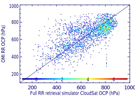
Figure 1 shows a comparison of the R3S-generated cloud OCP with OMI RRS cloud OCP retrievals. We used 2972 CloudSat 2B-TAU profiles from 13 November 2006 for this comparison. Note that the 2B-GEOPROF-LIDAR prod-uct was not available on this day, so the check for missed low-level clouds is not performed in this comparison or in the similar comparison with a fast simulator in Sect. 4.3. There is generally good agreement, although OMI RRS retrievals are biased low by approximately 75 hPa for high pressure (low altitude) clouds that dominate the population. There is also a branch of OMI RRS retrievals with higher OCPs than those

200 400 600 800 1000

Full RR retrieval simulator CloudSat OCP (hPa) 200

400 600 800 1000

OMI RR OCP (hPa)

0 2 4 6 8

Fig. 1. Two dimensional (2-D) histogram comparing cloud OCPs

from the OMI rotational-Raman scattering retrievals with those from the full rotational-Raman scattering simulator (R3S) using CloudSat extinction profiles withτ >5 for a single day (13 Novem-ber 2006). Results are provided as 2 dimensional densities in cloud pressure bins of 10 hPa. The color scale represents the number of observations falling within a given bin.

from the R3S CloudSat simulation. We examine these situa-tions in more detail below.

4 Fast cloud optical centroid pressure (OCP) simulators

4.1 Cloud OCP formulations

The cloud OCP, within the context of the Lambertian-Equivalent Reflectivity (LER) model, is defined as the pres-sure at which a Lambertian surface is placed to provide the observed amount of absorption (e.g., from oxygen) or filling-in due to rotational-Raman scatterfilling-ing. The Mixed LER (MLER) model further specifies a weighting of clear and cloudy subpixels with the effective cloud fraction as given by Eq. (1). The resulting cloud pressure,POCP, can be used to approximate the mean photon pathlength of a more com-plex scenario in which there could be partial or thin clouds and the clouds themselves may be geometrically thick and inhomogeneous (e.g., Koelemeijer et al., 2001; Vasilkov et al., 2008; Stammes et al., 2008; Ziemke et al., 2009).

(6)

a cloud layerLat a mean pressurePLundergoes an amount of absorption that is proportional to1PL, where1PLis the layer thickness from the top of the atmosphere (P0= 0) to pressurePL(1PL=PL).

For a given cloud or aerosol optical extinction profile, one may compute cloud/aerosol layer reflectances and trans-mittances, rL and tL, respectively, from a layer L using, for example, a two-stream model. Here, we use the delta-Eddington approximation of Joseph et al. (1976) with diffuse illumination to compute the layer reflectances and transmit-tances from elastic scattering (rotational-Raman scattering is not included). The delta-Eddington approximation provides accurate reflectances and transmittances over a wide range of conditions (errors<2 % for SZA<about 66◦increasing to a maximum of 15 % as SZA approaches 84◦). Errors will be smaller for geometrically thick clouds where the dependence upon SZA is mitigated as light becomes more diffuse inside the cloud. The delta-Eddington approximation therefore ap-pears to be appropriate for providing relative values of layer reflectances and transmittances (with respect to one another) that are most important for estimating the cloud OCP.

We then compute a reflectance contribution, ρL, from layerLto the total cumulative reflectance using

ρL =

rLT_L2−1 (1 −RL−1rL)

, (2)

whereRL andTLare cumulative reflectances and transmit-tances, respectively, from the top-of-atmosphere to layerL, given by

RL = L X

l=1

ρl (3)

and TL =

TL−1tL 1 −RL−1rL

, (4)

andT0= 1,R0= 0.

The cloud OCP (POCP) may then be approximated as a weighted-average over all layers from the top-of-atmosphere to the surface, where the weighting factor is given byρL, i.e.,

POCP ' P

l ρlPl

P

l ρl

. (5)

This formulation would produce an observed amount of absorption weighted by the same factor, i.e., an amount of absorption equivalent to that obtained when a single geometrically-thin, optically-thick cloud layer is placed at a pressure ofPOCP.

We tested several other methods for computing layer re-flectances and transmittances such as those from Coakley and Chylek (1975) and Meador and Weaver (1980) with dif-ferent input parameters. All methods provided very simi-lar OCP values; although absolute reflectances and transmit-tances may be somewhat different for the different methods,

the relative values as a function of layer, did not differ sub-stantially. For example, correlation coefficients computed with respect to exact simulator calculations for the Cloud-Sat profiles used in Sect. 3 varied within±0.05 and biases within±20 hPa for the suite of radiative transfer models and input parameters tested. We also compared OCPs computed with single scattering albedos of 1.0 and 0.99. Again, the relative values of layer reflectances/transmittances did not change enough to make significant differences (i.e., more than a few hPa) in computed cloud OCPs.

The standard fast simulator may also be modified to ac-count for properties of different types of cloud OCP re-trievals. For example, the weighting scheme may be mod-ified to simulate a cloud OCP from a retrieval based on an absorber with a pressure-squared dependence (P_OCP0 ) such as the oxygen dimer, e.g.,

P_OCP0 ' v u u u u t

P

l ρlP_l2

P

l ρl

. (6)

We compared OCPs computed with the standard (Eq. 5) and pressure-squared (Eq. 6) formulations using profiles from one day of CloudSat data. We found that the pressure-squared formulation gave OCPs on average about 7 hPa higher (lower altitude) than the standard formulation with a standard deviation of 11 hPa and a maximum difference of 101 hPa.

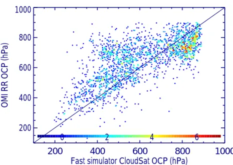
4.2 Comparison of fast and full cloud OCP simulators

Figure 2 compares the standard fast simulator results with those from the full rotational-Raman retrieval simulator (R3S) for the same sample of CloudSat profiles used above in Fig. 1. The R3S incorporates errors in the rotational-Raman cloud algorithm resulting from the use of the MLER model. Such errors have been previously reported by Vasilkov et al. (2008). These errors are largest for low cloud optical thick-nesses (<∼5). R3S results also account for the effects of en-hanced photon pathlengths due to Rayleigh scattering within clouds and between cloud layers that are not accounted for with the fast simulator. Considering the simplicity of the fast simulator and the errors present in R3S, the agreement be-tween the two is quite good, with a bias of 7.4 hPa, a standard deviation of 82 hPa, and a correlation coefficient of 0.89. 4.3 Single-day comparison of Cloudsat-based fast

simulator with OMI RRS retrievals

(7)

200 400 600 800 1000

Fast simulator CloudSat OCP (hPa) 200

400 600 800 1000

Full RR retrieval simulator CloudSat OCP (hPa

)

0 3 5 8 1

Fig. 2. 2-D histogram comparing cloud OCPs from the standard

fast simulator with those from the full rotational-Raman scattering simulator (R3S) for the same sample used in Fig. 1.

Fig. 2. R3S should better simulate OMI cloud RRS retrievals including errors owing to the use of the MLER model. We also see larger biases in the opposite direction for the lower pressure clouds. Again, this is consistent with expected bias in the fast simulator with respect to R3S. Although the full R3S provides a somewhat better agreement with OMI RRS retrievals than the fast simulator, the latter provides reason-able estimates of cloud OCP at a small fraction of the com-putational cost.

4.4 Cloud OCP weighting functions

In Eq. (5), ρ can be physically interpreted as a pressure weighting function. In other words, it weights a layerLwith mean pressurePL by the reflectance contribution from that layer,ρL. Next, we examine weighting functions calculated for one of the cloud scenarios used by Sneep et al. (2008) to investigate the behavior of four different cloud OCP al-gorithms; both the OMI RRS and O2-O2 algorithms were included as well as two O2-A band algorithms. In this ex-ample, the cloud is located between 550 and 800 hPa. As in Sneep et al. (2008), we use two different total cloud op-tical thicknesses,τ= 9 and 42, where the optical thickness is equally distributed within the cloud. Sneep et al. (2008) showed that all algorithms produced OCPs near the geomet-ric center of the cloud. For SZAs of 30◦and 40◦, view zenith angle (VZA) of 30◦, and relative azimuth angle of 90◦, cloud OCPs were slightly higher forτ= 9 as compared withτ= 42. For higher SZAs and VZAs, differences between theτ= 9 and 42 cases were smaller.

Figure 4 shows examples of weighting functions produced for the above scenarios along with the cloud OCPs produced by the standard fast simulator. For both cloud optical thick-nesses, the fast simulator places the cloud OCP in the middle of the cloud similar to the full simulations shown in Sneep et

200 400 600 800 1000

Fast simulator CloudSat OCP (hPa) 200

400 600 800 1000

OMI RR OCP (hPa)

0 2 4 6 8

Fig. 3. Similar to Fig. 1 but comparing cloud OCPs from the OMI rotational-Raman retrievals with those from the standard fast simulator.

0.00 0.05 0.10 0.15 0.20 0.25

Normalized weighting function 1000

800 600 400 200

Pressure (hPa)

Cloud top

Cloud base

uniform cloud optical thickness Total optical thickness = 9

fast simulator OCP = 642 hPa

Total optical thickness = 42

fast simulator OCP = 605 hPa

Fig. 4. Cloud OCPs and weighting functions for clouds with a

uniform optical extinction profile and two different total optical thicknesses.

al. (2008). As expected, the fast simulator shows more pho-ton penetration for theτ= 9 case. For theτ= 42 case, the fast simulator cloud OCP is weighted more towards the top part of the cloud.

(8)

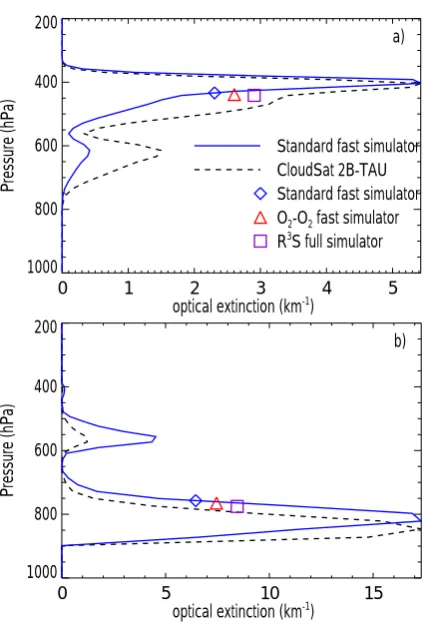
0 1 2 3 4 5 optical extinction (km-1)

1000 800 600 400 200

Pressure (hPa)

a)

Standard fast simulator CloudSat 2B-TAU Standard fast simulator O2-O2 fast simulator R3S full simulator

0 5 10 15

optical extinction (km-1) 1000

800 600 400 200

Pressure (hPa)

b)

Fig. 5. Two examples of CloudSat cloud extinction profiles (dashed

curves), corresponding cloud OCPs computed with different simu-lators (symbols as indicated, offset on the x-axis for clarity), and weighting functions computed using the standard fast simulator (blue solid curves).

Figure 6 shows examples where OCP differences between the fast simulators and R3S are larger, and one case where the difference between standard and pressure-squared (O2-O2) weighting in the fast simulators is also significant. The pro-file in Fig. 6a shows a case where the upper layer has a large optical thickness (∼50). The cloud OCP weighting function peaks at a higher altitude than the cloud extinction profile. The standard fast cloud OCP simulation is close to the peak in the weighting function in the upper cloud deck; there is not much sensitivity of the cloud OCP to the lower cloud deck. The standard and pressure-squared weightings provide similar results in this case. The full R3S cloud OCP simu-lation is almost 150 hPa higher than the estimates from the fast simulators. This difference presumably results from en-hanced photon pathlengths due to Rayleigh scattering within the cloud that is not accounted for in the fast simulators.

Figure 6b shows an example where the standard and pressusquared weightings provide slightly different re-sults. This is another multi-layer cloud case, but here the top layer has a lower optical thickness (∼6). As a result, the weighting function shows significant sensitivity to the lower cloud deck. As expected, the pressure-squared weighting

0 5 10 15 20

optical extinction (km-1) 1000

800 600 400 200

Pressure (hPa)

Standard fast simulator CloudSat 2B-TAU

Standard fast simulator O2-O2 fast simulator R3

S full simulator a)

0 5 10 15

optical extinction (km-1 ) 1000

800 600 400 200

Pressure (hPa)

b)

Fig. 6. Similar to Fig. 5; Two examples of CloudSat cloud

extinc-tion profiles for multi-layer clouds: (a) case with an optically thick upper layer (τ'50); (b) case with an optically thin upper layer (τ'6). Standard and O2-O2fast simulator results are more

simi-lar for the optically thick upper layer; O2-O2weights more heavily

towards the lower layer when the upper layer is more optically thin.

provides more sensitivity to the lower cloud deck (higher pressure) than that from the standard weighting. Both fast cloud OCP simulations provide a value in the middle of the two cloud decks, with the pressure-squared weighting about 75 hPa higher. The full R3S provides a higher value of cloud OCP than both fast simulations, presumably because it ac-counts for Rayleigh scattering between the cloud layers.

5 Monthly comparisons of CloudSat-based fast simulator OCPs with OMI retrievals

The fast simulators make it more computationally feasible to do a large number of comparisons with CloudSat under a wide range of conditions. Such comparisons may reveal spe-cific problems with the cloud OCP retrievals. However, in all comparisons of this type, we must bear in mind the expected differences between the fast simulators and the retrievals as shown for the RRS retrievals in Fig. 2.

(9)

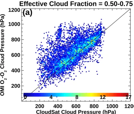
Effective Cloud Fraction = 0.50-0.75

200 400 600 800 1000 1200

CloudSat Cloud Pressure (hPa) 200

400 600 800 1000 1200

OMI RRS Cloud Pressure (hPa)

0 3 6 9 13

(a)

Effective Cloud Fraction = 0.75-1.00

200 400 600 800 1000 1200

400 600 800 1000 1200

0 5 10 15 20

(b)

Fig. 7. Comparison of cloud pressures using a 2-D histogram as in

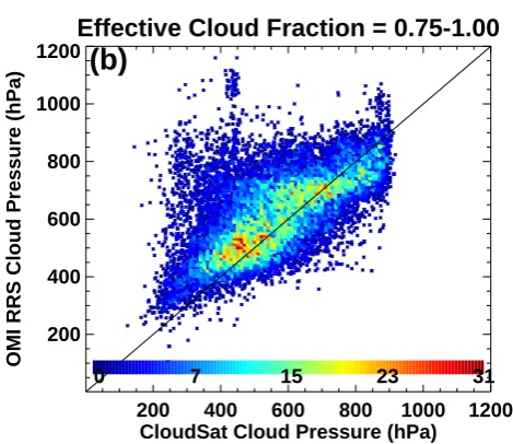
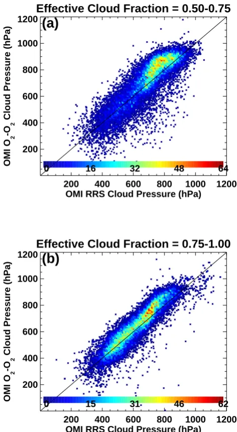
Fig. 2: CloudSat OCPs (based on 2B-TAU profiles and the standard fast simulator) with OMI RRS cloud OCP retrievals over land for different bins of effective cloud fraction for July 2007. Note that the color scale changes for the different effective cloud fraction bins.

two months (January and July 2007). OMI RRS retrievals will be compared with results from the standard simulator and those from O2-O2 will be compared with results from the pressure-squared formulation. In this set of comparisons, we use a different scheme for averaging CloudSat data along the track for the length of the OMI FOV. Here, we compute a cloud OCP using our fast simulators (standard and pressure-squared versions) for each cloudy CloudSat sounding with totalτ >0.1 that falls within an OMI FOV. We then compute a reflectance-weighted average OCP over the corresponding CloudSat pixels. We believe this method to be more accurate

Effective Cloud Fraction = 0.50-0.75

200 400 600 800 1000 1200

400 600 800 1000 1200

OMI O

2

-O

2

Cloud Pressure (hPa)

0 4 8 12 17

(a)

Effective Cloud Fraction = 0.75-1.00

200 400 600 800 1000 1200

400 600 800 1000 1200

OMI O

2

-O

2

0 5 11 16 22

(b)

Fig. 8. Similar to Fig. 7 but for OMI O2-O2cloud OCP retrievals

(over land, July 2007).

than averaging optical thicknesses of CloudSat profiles over the length of the OMI pixel as was done in Sect. 3. Never-the-less, differences between the two averaging methods are small; for a single day of CloudSat profiles with total opti-cal thicknesses>5, the mean difference in cloud OCP was 3.6 hPa with a standard deviation of 8.3 hPa.

5.1 Comparisons with CloudSat-based fast simulators over land

(10)

Table 1. Monthly-mean cloud OCP comparison statistics including

average(mean) difference, standard deviation of the difference (σ), both in hPa, and correlation coefficient,R, for July 2007, where CS stands for OCPs from CloudSat profiles run through the fast simulators.

0.50< feff<0.75 0.75< feff<1.0

Data sets, avg. σ R avg. σ R

conditions diff. diff. Land

RRS-CS 41 143 0.59 72 122 .64 O2O2-CS 70 132 0.66 102 121 .65

RRS-O2O2 −33 87 0.84 −36 62 .90

Ocean

RRS-CS 36 144 0.65 52 125 .64 O2O2-CS 59 143 0.68 68 128 .65

RRS-O2O2 −28 86 0.86 −24 62 .92

used for all subsequent figures to provide the same sample for comparisons and computed statistics. Statistics for these and other comparisons are provided in Table 1.

There is reasonable agreement between CloudSat-simulated OCPs and those from both OMI algorithms. Slight biases between CloudSat and OMI RRS OCPs resemble those shown earlier that are produced from inconsistencies between OMI retrievals and the fast simulators. However, as was also shown in Fig. 1, there is a cluster of retrievals with CloudSat-based OCPs near 400 hPa for which both OMI al-gorithms retrieve significantly higher pressures. The differ-ences are larger than those expected from the fast simulators. The reduced scatter at higher effective cloud fractions can be explained as follows: Both random and systematic errors in the cloud OCP retrievals are amplified by a factor that is inversely proportional to the cloud radiance fraction (fr), de-fined as the fraction of observed radiance that is due to scat-tering from cloud particles. Errors in cloud OCP become large asfrapproaches zero. The cloud radiance fraction can be estimated within the MLER context (see Eq. 1) using

fr = feff Icld Iobs

. (7)

While Icld is relatively constant with wavelength (at the wavelengths considered here), Iobs is wavelength depen-dent owing to variations in Rayleigh scattering and surface albedo. The much brighter Rayleigh scattering background in the UV (as compared with the visible) results in lower val-ues offrfor the OMI RRS retrievals as compared with those from the O2-O2for a given value offeff. Therefore, we ex-pect greater error amplification for the RRS retrievals at low values offeff. Indeed, we observe slightly higher correlations between CloudSat and OMI O2-O2than for Cloudsat versus OMI RRS in the lowerfeffbin. At the wavelengths used for

Effective Cloud Fraction = 0.50-0.75

200 400 600 800 1000 1200

400 600 800 1000 1200

0 14 29 44 59

(a)

Effective Cloud Fraction = 0.75-1.00

200 400 600 800 1000 1200

400 600 800 1000 1200

0 7 15 23 31

(b)

Fig. 9. Similar to Fig. 7 but over ocean (July 2007).

the OMI RRS retrieval,fr'2feff forfeff<∼0.3. Errors at feff= 5 % are thus about an order of magnitude higher than those at 100 %. In this paper we focus on data with moderate to high values of cloud radiance fraction.

(11)

Effective Cloud Fraction = 0.50-0.75

200 400 600 800 1000 1200

400 600 800 1000 1200

OMI O

2

-O

2

0 27 55 82 110

(a)

Effective Cloud Fraction = 0.75-1.00

200 400 600 800 1000 1200

400 600 800 1000 1200

OMI O

2

-O

2

0 8 17 25 34

(b)

Fig. 10. Similar to Fig. 9 but for O2-O2(ocean, July 2007).

set. Analysis of these cases shows that the snow flag is set on subsequent days. We also found a few isolated areas where snow is likely (e.g., northern Canada in winter) and the snow/ice flag is not set, while it is set for the surrounding region.

Not all discrepancies between CloudSat and OMI cloud OCPs occurred near regions of snow-ice. An examination of the CloudSat profiles showed that many of these locations contained multi-layered clouds. As shown in Fig. 6, these are the profiles for which the standard fast simulator has the largest differences with the full RRS simulator. The differ-ences, however, are generally too large to be explained by the fast simulator alone. In many cases, multiple outliers occur within a close proximity where there is significant variabil-ity in the CloudSat-simulated cloud OCP as well as cloud-top

Effective Cloud Fraction = 0.50-0.75

200 400 600 800 1000 1200

OMI RRS Cloud Pressure (hPa) 200

400 600 800 1000 1200

OMI O

2

-O

2

0 5 10 15 20

(a)

Effective Cloud Fraction = 0.75-1.00

200 400 600 800 1000 1200

400 600 800 1000 1200

OMI O

2

-O

2

0 14 29 43 58

(b)

Fig. 11. Similar to Fig. 7 (same sample of observations) but

compar-ing OMI cloud OCP retrievals from the RRS and O2-O2products

over land (July 2007).

(12)

Effective Cloud Fraction = 0.50-0.75

200 400 600 800 1000 1200

400 600 800 1000 1200

OMI O

2

-O

2

0 16 32 48 64

(a)

Effective Cloud Fraction = 0.75-1.00

200 400 600 800 1000 1200

400 600 800 1000 1200

OMI O

2

-O

2

0 15 31 46 62

(b)

Fig. 12. Similar to Fig. 11 (same sample of observations) but over

ocean (July 2007).

5.2 Comparisons with CloudSat-based fast simulators over ocean

Figures 9–10 show comparisons similar to those in Figs. 7– 8, but over ocean. Here, we see a predominance of low altitude (high pressure) clouds for moderate values offeff. A bimodal distribution in the low clouds with peaks near 775 and 875 hPa is apparent forfeff between 50 and 75 %. This bimodality, a prevalent feature of trade wind cumulus clouds, has been observed in several different passive satel-lite cloud-top height data sets, both thermal IR and stereo algorithms, as well as surface ceilometer cloud base height measurements (e.g., Genkova et al., 2007; Mote and Frey, 2006). High altitude (low pressure) clouds are prevalent only

Ocean

200 400 600 800 1000

Cloud Pressure for ECF>0.3 0.00

0.01 0.02 0.03 0.04 0.05

Fraction

CloudSat

OMI RRS OMI O2-O2

(a)

Land

200 400 600 800 1000

Cloud Pressure for ECF>0.3 0.00

0.01 0.02 0.03 0.04 0.05

Fraction

(b)

Fig. 13. Probability distribution functions of CloudSat cloud OCP

(2B-TAU profiles with fast simulators) and the two OMI cloud al-gorithms over ocean (a) and land (b) for observations with effective cloud fraction (ECF)>0.3.

for high effective cloud fractions. As over land, though not as distinct, for both OMI algorithms we see a cluster of points with a higher cloud OCP than predicted from CloudSat 2B-TAU and the fast simulators.

5.3 Comparisons of two OMI cloud algorithms over land and ocean

Figures 11 and 12 show similar 2-D histograms for the same sample of observations as above, but now for the OMI RRS versus O2-O2cloud OCPs over land and ocean, respectively. The O2-O2 OCPs are slightly higher than those from RRS retrievals on average. The distributions are skewed, particu-larly over ocean where the O2-O2algorithm provides higher cloud OCPs than those from the RRS algorithm.

(13)

-135 -90 -45 0 45 90 135

-60

-30

0

30

60

-60

-30

0

30

60

(a)

<0.05 0.15 0.30 0.45 0.60 0.75 >0.9 Effective Cloud Fraction

-135 -90 -45 0 45 90 135

-60

-30

0

30

60

-60

-30

0

30

60

(b)

<300 400 500 600 700 800 >900 CloudSat Cloud Pressure (hPa)

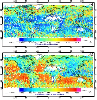
Fig. 14. Maps of gridded effective cloud fraction from the OMI cloud RRS algorithm (a) and cloud OCP from CloudSat (b) for July 2007.

reflectance values, while there was only a slight sensitivity of cloud pressure retrievals in the oxygen A-band to cloud 3-D effects. However, they simulated only a few scenarios. The cloud adjacency effect (Marshak et al., 2008) may be important for OMI cloud OCP retrievals.

5.4 Probability Distribution Functions (PDFs) of cloud OCP

Figure 13 shows cloud OCPs from OMI and CloudSat (stan-dard weighting) for July 2007 displayed as probability dis-tribution functions (PDFs) for both land and ocean and de-rived using only observations withfeff>0.3. The OMI dis-tributions are similar to those shown previously by Sneep et al. (2008). Over ocean, CloudSat shows a trimodal distribu-tion with a small peak near 400 hPa. Both OMI algorithms only hint at a low pressure mode, with a higher pressure than that given by CloudSat. As noted earlier for high pres-sure clouds, there are peaks in the distribution near 775 and 875 hPa in the CloudSat-derived OCPs. The OMI RRS algo-rithm underestimates the pressure of these clouds while the OMI O2-O2 algorithm overestimates. Neither OMI cloud

algorithm shows a clear bimodal distribution in the high pressure clouds, though there is a hint of bimodality in the OMI RRS PDF. Genkova et al. (2007) showed that distri-butions of cloud top heights of trade wind cumulus derived from thermal IR measurements are affected by spatial resolu-tion. It should be noted that the OMI FOV is twice as wide in the cross-track direction as the length along track over which the CloudSat OCPs are averaged.

(14)

0 5 10 15 20 25 30

Data Points (%)

-1000 -500

-500 -250

-250 -150

-150 -50

-50 50

50 150

150 250

250 500

500 1000

N=29849 (a)

CloudSat-fast Sim. OCP - OMI RR OCP (hPa)

July 2007 (b)

Fig. 15. Histogram (a) and color-coded map (b) of differences

be-tween CloudSat cloud OCP and that from the OMI RRS algorithm for effective cloud fractions>0.1.

5.5 Maps of cloud OCP and effective cloud fraction

Figure 14 shows gridded maps offeff from the OMI RRS algorithm and cloud OCP from CloudSat for the observa-tions collocated with CloudSat in July 2007. This provides a context for maps of the differences between CloudSat-based OCPs and those from OMI RRS and O2-O2, respectively, shown in Figs. 15 and 16. These figures also show corre-sponding histograms. The difference maps show all individ-ual points (i.e., not gridded data). Each point is color-coded by the corresponding histogram bin. Note that we include all observations withfeff as low as 0.1; at these low values of feff, error amplification can be substantial and is larger for the OMI RRS results than for O2-O2.

In the histograms, the skewed distributions are seen here for both OMI algorithms versus CloudSat over land and ocean as shown in previous figures. The maps provide the geographic distribution of the differences. It is now appar-ent that most of the positive differences (CloudSat OCPs higher than OMI) over ocean occur in regions where sub-sidence produces low clouds and relatively low values of feff. The OMI RRS algorithm produces larger positive dif-ferences in these regions than the O2-O2. The high cloud OCPs seen in the inter-tropical convergence zone (ITCZ) show mostly negative differences (Cloudsat OCPs lower than those from both OMI algorithms). Some differences be-tween OMI algorithms are seen such as over the Pacific at low latitudes where Joiner et al. (2010) showed that large numbers of OMI FOVs contain multi-layer clouds. Finally,

0 5 10 15 20 25 30

Data Points (%)

-1000 -500

-500 -250

-250 -150

-150 -50

-50 50

50 150

150 250

250 500

500 1000

N=29849 (a)

CloudSat-fast Sim. OCP - OMI O

2-O2 OCP (hPa)

July 2007 (b)

Fig. 16. Similar to Fig. 15, but for OMI O2-O2.

we note alternating patterns of differences between Cloud-Sat and OMI RRS with latitude at the high southern lati-tudes where solar zenith angles are highest. This may in-dicate some residual errors in the look-up table interpolation scheme. Such patterns are muted in the O2-O2 results that have been recently updated with more nodes added to the ta-ble look-up scheme.

We also examined data for January 2007. The spatial pat-terns of differences with CloudSat are similar to July in the tropics. At moderate to high latitudes, the patterns have re-versed with respect to the hemispheres. Comparison of the differences in both July and January 2007 are qualitatively consistent with those expected from missed low clouds that are maximum in the summer hemisphere at moderate to high latitudes as shown by Stephens et al. (2008).

6 Conclusions

We have developed a relatively simple scheme for simulating retrieved cloud optical centroid pressures from satellite so-lar backscatter observations. We compared fast simulator re-sults with those from a detailed retrieval simulator that more fully accounts for the complex radiative transfer in a cloudy atmosphere; agreement is reasonable between the two. We also showed several examples of weighting functions for the cloud OCP.

(15)

We find that both OMI algorithms perform reasonably well, and that the two algorithms agree better with each other than either does with the collocated CloudSat data. This indicates that patchy snow/ice, cloud 3-D effects, and/or uncertainties both in the CloudSat 2B-TAU profiles and fast simulators are affecting comparisons with both OMI products similarly.

Our fast simulators may be used to simulate cloud OCP from output generated by general circulation models (GCM) with appropriate account of cloud overlap. We have imple-mented such a scheme and plan to compare OMI data with GCM output in the near future. Fast simulators are also ideal for assimilation of satellite-derived OCPs where computa-tional efficiency is important. For these applications, uncer-tainties and errors in both the fast simulators and OMI OCP retrievals must be accounted for. This work provides a basis for estimating those uncertainties.

Acknowledgements. This material is based upon work supported

by the National Aeronautics and Space Administration under agreement NNH10ZDA001N-AURA issued through the Science Mission Directorate for the Aura Science Team managed by Kenneth Jucks and Richard Eckman. We thank the OMI, MODIS, and CloudSat data processing teams for providing the data used for this study. We thank the two anonymous reviewers whose com-ments led to improvecom-ments in the final version of the manuscript and associate editor Bernhard Mayer. The lead author thanks Arlindo da Silva for helpful discussions that include coining the term “optical centroid pressure”.

Edited by: B. Mayer

References

Acarreta, J. R., de Haan, J. F., and Stammes, P.: Cloud pressure retrieval using the O2-O2absorption band at 477 nm, J. Geophys.

Res., 109, D05204, doi:10.1029/2003JD003915, 2004.

Ahmad, Z., Bhartia, P. K., and Krotkov, N.: Spectral properties of backscattered UV radiation in cloudy atmospheres, J. Geophys. Res., 109, D01201, doi:10.1029/2003JD003395, 2004.

Baum, B. A., Yang, P., Heymsfield, A. J., Platnick, S., King, M. D., Hu, Y. X., and Bedka, S. T.: Bulk scattering models for the re-mote sensing of ice clouds, Part 2: Narrowband models, J. Appl. Meteorol., 44, 1896–1911, 2005.

Bovensmann, H., Burrows, J., Buchwitz, M., Frerick, J., Noel, S., Rozanov, V., Chance, K., and Goede, A.: SCIAMACHY: mission objectives and measurement modes, J. Atmos. Sci., 56, 127–150, 1999.

Boersma, K. F., Eskes, H. J., and Brinksma, E. J.: Error analysis for tropospheric NO₂ retrieval from space, J. Geophys. Res., 109, D04311, doi:10.1029/2003JD003962, 2004.

Bucsela, E. J., Celarier, E. A., Wenig, M. O., Gleason, J. F., Veefkind, J. P., Boersma, K. F., and Brinksma, E. J.: Algorithm for NO2 vertical column retrieval from the Ozone Monitoring

Instrument, IEEE T. Geosci. Remote, 44, 1245–1258, 2006. Burrows, J. P., Weber, M., Buchwitz, M., Rozanov, V.,

Ladstatter-Weissenmayer, A., Richter, A., deBeek, R., Hoogen, R., Bram-stedt, K., Eichmann, K.-U., Eisinger, M., and Perner, D.: The

Global Ozone Monitoring Experiment (GOME): Mission con-cept and first scientific results, J. Atmos. Sci., 56, 151–175, 1999. Chang F.-L. and Li, Z.: A new method for detection of cirrus over-lapping water clouds and determination of their optical proper-ties, J. Atmos. Sci., 62, 3993–4009, 2005a.

Chang F.-L. and Li, Z.: A near-global climatology of single-layer and overlapped clouds and their optical properties retrieved from Terra/MODIS data using a new algorithm, J. Climate, 18, 4572– 4771, 2005b.

CloudSat Project: Level 2 cloud optical depth product process description and interface control document, version 5.0, avail-able at: http://www.cloudsat.cira.colostate.edu/ICD/2B-TAU/ 2B-TAU PDICD 5.0.pdf, last access: 4 October 2011, Colorado State University, Fort Collins, CO, USA, 2008.

Coakley, J. A. and Chylek, P.: The two-stream approximation in the radiative transfer: Including the angle of incident radiation, J. Atmos. Sci., 32, 409–418, 1975.

Coldewey-Egbers, M., Weber, M., Lamsal, L. N., de Beek, R., Buchwitz, M., and Burrows, J. P.: Total ozone retrieval from GOME UV spectral data using the weighting function DOAS approach, Atmos. Chem. Phys., 5, 1015–1025, doi:10.5194/acp-5-1015-2005, 2005.

Comstock, J. M. and Jakob, C.: Evaluation of tropical cirrus cloud properties derived from ECMWF model output and ground based measurements over Nauru Island, Geophys. Res. Lett., 31, L10106, doi:10.1029/2004GL019539, 2004.

Cox, C. and Munk, W.: Measurement of the roughness of the sea surface from photographs of the Sun’s glitter, J. Opt. Soc. Am., 44, 838–850, 1954.

Daniel, J. S., Solomon, S., Miller, H. L., Langford, A. O., Port-mann, R. W., and Eubank, C. S.: Retrieving cloud informa-tion from passive measurements of solar radiainforma-tion absorbed by molecular oxygen and O2-O2, J. Geophys. Res., 108, 4515,

doi:4510.1029/2002JD002994, 2003.

Deirmendjian, D.: Electromagnetic scattering on spherical polydis-persions, Elsevier Sci., New York, 290 pp., 1969.

Dubuisson, P., Frouin, R., Dessailly, D., and Duforet, L,: Altitude of aerosol plumes over the ocean from reflectance ratio measure-ments in the O2 A-band, Remote Sens. Environ., 113, 1899–

1911, 2009.

Ferlay, N., Thieuleux, F., Cornet, C., Davis, A. B., Dubuis-son, P., Ducos, F., Parol, F., Ri´edi, J., and Vanbauce, C.: Toward New Inferences about Cloud Structures from Multi-directional Measurements in the Oxygen A Band: Middle-of-Cloud Pressure and Cloud Geometrical Thickness from POLDER-3/PARASOL, J. Appl. Meteorol. Clim., 49, 2492– 2507, doi:10.1175/2010JAMC2550.1, 2010.

Genkova, I., Seiz, G., Zuidema, P., Zhao, G., and Di Girolamo, L.: Cloud top height comparisons from ASTER, MISR, and MODIS for trade wind cumuli, Remote Sens. Environ., 107, 211–222, 2007.

Joiner, J. and Bhartia, P. K.: Accurate Determination of Total Ozone using SBUV Continuous Spectral Scan Measurements, J. Geo-phys. Res., 102, 12957–12969, 1995.

Joiner, J. and Vasilkov, A. P.: First results from the OMI rotational raman scattering cloud pressure algorithm, IEEE T. Geosci. Re-mote, 44, 1272–1282, 2006.

(16)

scattering in GOME spectra, J. Geophys. Res., 109, D01109, doi:10.1029/2003JD003698, 2004.

Joiner, J., Vasilkov, A. P., Yang, K., and Bhartia, P. K.: Total column ozone over hurricanes from the ozone monitoring instrument, Geophys. Res. Lett., 33, L06807, doi:10.1029/2005GL025592, 2006.

Joiner, J., Schoeberl, M. R., Vasilkov, A. P., Oreopoulos, L., Plat-nick, S., Livesey, N. J., and Levelt, P. F.: Accurate satellite-derived estimates of the tropospheric ozone impact on the global radiation budget, Atmos. Chem. Phys., 9, 4447–4465, doi:10.5194/acp-9-4447-2009, 2009.

Joiner, J., Vasilkov, A. P., Bhartia, P. K., Wind, G., Platnick, S., and Menzel, W. P.: Detection of multi-layer and vertically-extended clouds using A-train sensors, Atmos. Meas. Tech., 3, 233–247, doi:10.5194/amt-3-233-2010, 2010.

Joseph, J. H., Wiscombe, W. J., and Weinman, J. A.: The delta-Eddington approximation for radiative flux transfer, J. At-mos. Sci., 33, 2452–2459, 1976.

Koelemeijer, R. B. A. and Stammes, P.: Effects of clouds on ozone column retrieval from GOME UV measurements, J. Geophys. Res., 104, 8281–8294, 1999.

Koelemeijer, R. B. A., Stammes, P., Hovenier, J. W., and de Haan, J. F.: A fast method for retrieval of cloud parameters using oxy-gen A-band measurements from the Global Ozone Monitoring Experiment, J. Geophys. Res., 106, 3475–3496, 2001.

Koelemeijer, R. B. A., Stammes, P., Hovenier, J. W., and de Haan, J. F.: Global distribution of effective cloud fraction and cloud top pressure derived from oxygen A band measured by the Global Ozone Monitoring Experiment: Comparison to ISCCP data, J. Geophys. Res., 107, 4151, doi:10.1029/2001JD000840, 2002. Kokhanovsky, A. A., Rozanov, V. V., Nauss, T., Reudenbach, C.,

Daniel, J. S., Miller, H. L., and Burrows, J. P.: The semianalytical cloud retrieval algorithm for SCIAMACHY I, The validation, At-mos. Chem. Phys., 6, 1905–1911, doi:10.5194/acp-6-1905-2006, 2006.

Kokhanovsky, A. A., Mayer, B., Rozanov, V. V., Wapler, K., Bur-rows, J. P., and Schumann, U.: The influence of broken cloudi-ness on cloud top height retrievals using the nadir observations of backscattered solar radiation in the oxygen A-band, J. Quant. Spectrosc. Ra., 103, 460–477, 2007a.

Kokhanovsky, A. A., Mayer, B., Rozanov, V. V., Wapler, K., Lam-sal, L. N., Weber, M., Burrows, J. P., and Schumann, U.: Satellite ozone retrieval under broken cloud conditions: An error analysis based on Monte Carlo simulations, IEEE T. Geosci. Remote, 45, 187–194, 2007b.

L’Ecuyer, T. S., Wood, N. B., Haladay, T., Stephens, G. L., and Stackhouse Jr., P. W.: Impact of clouds on atmospheric heating based on the R04 CloudSat fluxes and heating rates data set, J. Geophys. Res., 113, D00A15, doi:10.1029/2008JD009951, 2008.

Levelt, P. F., van der Oord, G. H. J., Dobber, M. R., Malkki, A., Visser, H., de Vries, J., Stammes, P., Lundell, J. O. V., and Saari, H.: The ozone monitoring instrument, IEEE T. Geosci. Remote, 44, 1093–1101, 2006.

Mace, G. G., Zhang, Q., Vaughan, M., Marchand, R., Stephens, G., Trepte, C., and Winker, D.: A description of hydrometeor layer occurrence statistics derived from the first year of merged Cloudsat and CALIPSO data, J. Geophys. Res., 114, D00A26, doi:10.1029/2007JD009755, 2009.

Marshak, A., Davis, A., Wiscombe, W., Ridgway, W., and Cahalan, R.: Biases in shortwave column absorption in the presence of fractal clouds, J. Climate, 11, 431–446, 1998.

Marshak, A., Wen, G., Coakley, J. A., Remer, L. A., Loeb, N. G., and Cahalan, R. F.: A simple model for the cloud adjacency ef-fect and the apparent bluing of aerosols near clouds, J. Geophys. Res., 113, D14S17, doi:10.1029/2007JD009196, 2008. McPeters, R. D., Bhartia, P. K., Krueger, A. J., Herman, J. R.,

Schlesinger, B. M., Wellemeyer, C. G., Seftor, C. J., Jaross, G., Taylor, S. L., Swissler, T., Torres, O., Labow, G., Byerly, W., and Cebula, R. P.: Nimbus-7 Total Ozone Mapping Spectrome-ter (TOMS) data products user’s guide, NASA Ref. Pub. 1384, Washington, DC, USA, 67 pp., 1996.

Meador, W. E. and Weaver, W. R.: Two-stream approximation to radiative transfer in planetary atmospheres: A unified description of existing methods and a new improvement, J. Atmos. Sci., 37, 630–643, 1980.

Menzel, W. P., Frey, R., Zhang, H., Wylie, D. P., Moeller, C., Holz, R., Maddux, B., Baum, B. A., Strabala, K. I., and Gum-ley, L.: MODIS global cloud-top pressure and amount estima-tion: algorithm description and results, J. Appl. Meteorol. Clim., 47, 1175–1198, 2008.

Mote, P. W. and Frey, R.: Variability of clouds and water va-por in low latitudes: View from Moderate Resolution Imaging Spectroradiometer (MODIS), J. Geophys. Res., 111, D16101, doi:10.1029/2005JD006791, 2006.

Munro, R., Eisinger, M., Anderson, C., Callies, J., Corpaccioli, E., Lang, R., Lefebvre, A., Livschitz, Y., and Perez Albinana, A.: GOME-2 on Metop: from in-orbit verification to routine opera-tions, in: Proceedings of EUMETSAT Meteorological Satellite Conference, Helsinki, Finland, 12–16 June 2006.

Nolin, A., Armstrong, R. L., and Maslanik, J.: Near Real-Time SSM/I EASE-Grid Daily Global Ice Concentration and Snow Extent, January to March 2004 (updated daily), National Snow and Ice Data Center, Digital media, Boulder, CO, USA, 1998. Reuter, M., Buchwitz, M., Schneising, O., Heymann, J.,

Bovens-mann, H., and Burrows, J. P.: A method for improved SCIA-MACHY CO2retrieval in the presence of optically thin clouds,

Atmos. Meas. Tech., 3, 209–232, doi:10.5194/amt-3-209-2010, 2010.

Rozanov, V. V. and Kokhanovsky, A. A.: Semianalytical cloud re-trieval algorithm as applied to the cloud top altitude and the cloud geometrical thickness determination from top-of-atmosphere re-flectance measurements in the oxygen A band, J. Geophys. Res., 109, D05202, doi:10.1029/2003JD004104, 2004.

Rozanov, V. V., Kokhanovsky, A. A., and Burrows, J. P: The de-termination of cloud altitudes using GOME reflectance spectra: multilayered cloud systems, IEEE T. Geosci. Remote, 42, 1009– 1017, 2004.

Sneep, M., de Haan, J., Stammes, P., Wang, P., Vanbauce, C., Joiner, J., Vasilkov, A. P., and Levelt, P. F.: Three way comparison between OMI/Aura and POLDER/PARASOL cloud pressure products, J. Geophys. Res., 113, D15S23, doi:10.1029/2007JD008694, 2008.

(17)

Stammes, P., Sneep, M., de Haan, J. F., Veefkind, J. P., Wang, P., and Levelt, P. F.: Effective cloud fractions from the Ozone Moni-toring Instrument: Theoretical framework and validation, J. Geo-phys. Res., 113, D16S38, doi:10.1029/2007JD008820, 2008. Stephens, G. L., Vane, D. G., Taneli, S., Im, E., Durden, S., Rokey,

M., Reike, D., Partain, P., Mace, G. G., Austin, R., L’Ecuyer, T., Haynes, J., Lebsock, M., Suzuki, K., Waliser, D., Wu, D., Kay, J., Gettleman, A., Wang, Z., and Marchand, R.: CloudSat Mission: Performance and early science after the first year of operation, J. Geophys. Res., 113, D00A18, doi:10.1029/2008JD009982, 2008.

van Roozendael , M., Loyola, D., Spurr, R., Balis, D., Lam-bert, J.-C., Livschitz, Y., Valks, P., Ruppert, T., Kenter, P., Fayt, C., and Zehner, C.: Ten years of GOME/ERS-2 to-tal ozone data-The new GOME data processor (GDP) ver-sion 4: 1. Algorithm description, J. Geophys. Res., 111, D14311, doi:10.1029/2005JD006375, 2006.

Vanbauce, C., Cadet, B., and Marchand, R. T.: Compari-son of POLDER apparent and corrected oxygen pressure to ARM/MMCR cloud boundary pressures, Geophys. Res. Lett., 3, 1212, doi:10.1029/2002GL016449, 2003.

Vasilkov, A. P., Joiner, J., Yang, K., and Bhartia, P. K.: Improv-ing total column ozone retrievals by usImprov-ing cloud pressures de-rived from Raman scattering in the UV, Geophys. Res. Lett., 31, L20109, doi:10.1029/2004GL020603, 2004.

Vasilkov, A. P., Joiner, J., Spurr, R., Bhartia, P. K., Levelt, P. F., and Stephens, G.: Evaluation of the OMI cloud pressures derived from rotational Raman scattering by comparisons with other satellite data and radiative transfer simulations, J. Geophys. Res., 113, D15S19, doi:10.1029/2007JD008689, 2008.

Vasilkov, A. P., Joiner, J., Oreopoulos, L., Gleason, J. F., Veefkind, P., Bucsela, E., Celarier, E. A., Spurr, R. J. D., and Platnick, S.: Impact of tropospheric nitrogen dioxide on the regional radiation budget, Atmos. Chem. Phys., 9, 6389–6400, doi:10.5194/acp-9-6389-2009, 2009.

Veefkind, J. P., de Haan, J. F., Brinksma, E. J., Kroon, M., and Levelt, P.: Total ozone from the Ozone Monitoring Instrument (OMI) using the DOAS technique, IEEE T. Geosci. Remote, 44, 1239–1244, 2006.

Xi, B., Dong, X., Minnis, P., and Khaiyer, M. M.: A 10 year cli-matology of cloud fraction and vertical distribution derived from both surface and GOES observations over the DOE ARM SPG site, J. Geophys. Res., 115, D12124, doi:1029/2009JD012800, 2010.