https://doi.org/10.5194/os-14-1321-2018 © Author(s) 2018. This work is distributed under the Creative Commons Attribution 4.0 License.
Evaluation of extreme wave probability on the basis
of long-term data analysis
Kirill Bulgakov1,2, Vadim Kuzmin2, and Dmitry Shilov2
1Shirshov Institute of Oceanography, Russian Academy of Sciences, 36, Nahimovskiy prospekt, Moscow, 117997, Russia 2Russian State Hydrometeorogical University, 98, Maloochtinsky Pr., Saint Petersburg, 195196, Russia
Correspondence:Kirill Bulgakov ([email protected]) Received: 27 November 2017 – Discussion started: 16 January 2018
Revised: 6 October 2018 – Accepted: 12 October 2018 – Published: 25 October 2018
Abstract. A method of calculation of wind wave height probability based on the significant wave height probability is described (Chalikov and Bulgakov, 2017). The method can also be used for estimation of the height of extreme waves of any given cumulative probability. The application of the method on the basis of long-term model data is presented. Examples of averaged annual and seasonal fields of extreme wave heights obtained using the above method are given. Ar-eas where extreme waves can appear are shown.
1 Introduction
The highest risks of economic and environmental damage for sea-based human activities, i.e. cargo shipments, fishery, oil production etc., are mostly connected with extreme weather conditions on the sea surface, among which strong storms are the foremost. It is especially difficult to predict emergency situations caused by extreme waves for those cases of sea-based activities which require people’s long stay at sea or prolonged use of equipment in the ocean.
One of the methods to minimize possible risks is the use of climate data based on long-term series of observations. At present there are archives consisting of reanalysis data on surface waves based on wave forecasts corrected by differ-ent methods, i.e. direct measuremdiffer-ents using accelerometers and GPS buoys, remote measurements by satellite-borne al-timetry and various types of radars. The main characteris-tic of wave fields included in the archive is significant wave height Hs defined as a mean value (trough to crest) of one-third of the highest of all the waves (Ochi, 1998). The value ofHsis calculated in the following way:
Hs=4
∞ Z
0 ∞ Z
0
S kx, ky
dkxdky
1/2
, (1)
wherekx,kyare wave numbers, whileS(kx,ky)is the wave spectrum.
It is evident that knowledge on significant wave height is not sufficient to evaluate real wave height for a given wave field. Extreme waves of the same height can appear with different probability for different values of Hs. For exam-ple, a wave 10 m high can appear in both a wave field with
Hs=10 m and in a wave field withHs=5 m. Or there can be waves with a height of 15 and 17 m in a wave field char-acterized byHs=10 m. Thus,Hs data do not give enough information about the probability of real wave heights.
1322 K. Bulgakov et al.: Evaluation of extreme wave probability on the basis of long-term data analysis
straightforward. Contrary to such an approach, investigation of the statistics of wave height above mean level remains a subject of non-linear wave theory. From the practical point of view, for floating objects the data on the full height (trough to crest) of a wave are more important. However, the data on probability of wave height above mean level are important for fixed-construction offshore platforms.
The theoretical probability distribution for wave crest height (or wave height above mean level) was suggested by Weibull (1951). Later it was studied on a basis of observa-tional data in nature and wave channels (see review by Kharif et al., 2009). Extended data for estimation of probability of wave height can be obtained with integration of non-linear modes based on full equations for potential (irrotational) flow (Touboul and Kharif, 2010; Chalikov, 2009). Methods of probability calculations were considered in many papers (see, for example, Bitner-Gregersen and Toffoli, 2012; Dy-achenko et al., 2016).
The most popular method of trough-to-crest wave height detection is based on a zero-crossing technique. A direct method is based on the use of moving windows; the method is applicable for both 1-D and 2-D cases.
Estimation of extreme waves today is mostly made by analysis of data of significant wave height. Jiangxia (2018), analysing long-term data, considered that an extreme wave is a wave exceeding two significant wave heights. In Larsen et al. (2015) a long-term wave dataset was analysed using the spectral method, and it was shown that the spectrum of modelled significant wave height (trough to crest) con-tained the energy for a frequency of more than 2.5×10⁻⁵Hz (daily timescale and less). A spectral correction method was developed to fill in the missing variability in the modelled variable at high frequencies. In Guo and Sheng (2015) the peak-over-threshold method was used to estimate the ex-treme significant wave heights from 30-year wave simula-tions. In Samayam et al. (2017) estimation of extreme wave height (crest-mean level) was made by using methods of ex-treme value theory. The main advantage of the method of Chalikov and Bulgakov (2017) compared with methods men-tioned above is that their method is based on results of direct modelling of wave fields.
This paper is devoted to investigation of the statistics and geographical distribution of wave height above mean sea level.
2 Description of the method
In Chalikov and Bulgakov (2017) an algorithm for estimation of cumulative probability of wavesP (h)exceeding a specific value of wave height above mean level (h) was developed using long-term data onHs. The description of the method is given below.
The probability of a wave exceeding a specific height h, if significant wave height is in a small range dHsaroundHs,
equalsP (eH )e for specificHe=h/Hs multiplied by probabil-ity ofHs in this range (P (eH )e ·P (Hs)dHs), by the standard definition of conditional probability. Consequently,P (h)can be determined as the integral ofP (eH )e ·P (Hs)over all possi-ble values ofHs:
P (h)= Hsmax
Z
0
e
P (H )P (He s)dHs, (2)
whereP (Hs)is the probability distribution ofHsfor a spe-cific point, whileHsmaxis the maximum value ofHsin the dataset for a specific point.
The model Hs data used for P (Hs) (Significant wave dataset calculated by WaveWatch III, 2018) were calculated with the latest version of the WaveWatch III model (Tolman, 2014) and GFS-2 wind analysis 2 (Sasha et al., 2014). The hindcasts cover the period from August 1999 to July 2015. The spatial resolution of the dataset fields is 0.5◦×0.5◦. Cal-ibration of the model and its validation are carried out using a great number of wave buoys. The data and results of its validation are described in Chawla et al. (2013).
The approximation ofP (eH )e was based on results of a 3-D
model of potential (irrotational) flow. The model used spec-tral definitions of fields, finite differences for vertical deriva-tive calculation, and a fourth-order Runge–Kutta scheme for time integration. Fourier resolution is 256×64 wave numbers, and resolution in physical space is 1024×256 (more detail in Chalikov et al., 2014). The calculations were performed for 350 units of non-dimensional time, i.e. for 70 000 time steps. The initial conditions were generated on a basic JONSWAP spectrum. Model runs were calculated un-der the condition that input energy from wind to waves equals wave energy dissipation. This condition corresponds to fully developed wind waves. In total 75 experiments were made (more detail in Chalikov et al., 2014; Chalikov and Bulgakov, 2017).
The results of the series of experiments were processed in the following way: each wave field of surface height above mean level (η) reproduced by the numerical model was nor-malized by the value of significant wave height correspond-ing to this field (He=η/Hs). (Note thatηis a variable of the
3-D model of potential (irrotational) waves. It should be dis-tinguished fromhdespite the fact that bothηandhhave the same physical sense.) Then, a non-dimensional wave field was used for the calculation of cumulative probability of non-dimensional wave heightP (eH )e . The distribution obtained
was approximated by the following function:
e
P (H )e =exp
−3.97He−4.02He2
. (3)
Note thatP (eH )e is the cumulative probability of the height of
the free surface above mean level. This probability forHe=1
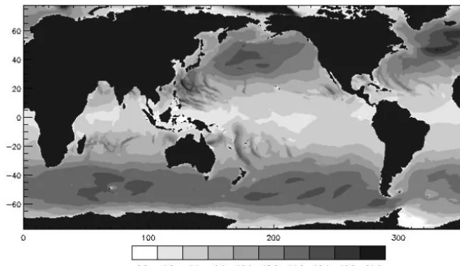
Figure 1.Wave heights (m) above mean level with a cumulative probability of 10−7, annual average.
The above expression can be used for the interval≤He≤
1.85. The probability of a wave higher than 1.85 (the maxi-mal value ofHein data) can be considered extremely low and
therefore is neglected. It should be noted that approximation (Eq. 3) was obtained with use of the precise 3-D model based on full non-linear equations. The volume of data used for ap-proximation (Eq. 3) include more than 4.5 billion values ofη
(number of points in a single field multiplied by the num-ber of records in the experiment multiplied by the numnum-ber of experiments). Currently, this approximation is considered universal for wind wave fields in which cases of freak waves are most likely. Waves of other types of spectrums (swells) have a small steepness and do not influence extreme wave generation except in cases in which long-wave currents can steepen shorter waves.
The spatial distribution of extreme wave probability was investigated, based on Eq. (3) from Chalikov and Bul-gakov (2017) together with the spatial distribution of signif-icant wave height from Chawla et al. (2013). In this paper results of an application of this method are considered. We show global fields of wave height with a cumulative proba-bility of 10−7thus calculated.
3 Results
Figure 1 shows an average annual field of wave heights with a cumulative probability of 10−7. It can be seen that waves with a height of up to 20 m above mean level can appear with such a probability, some of the extreme waves (16 m and more) being found in areas of active navigation (eastern part of the Atlantic Ocean, East China Sea, Philippine Sea, Yellow Sea, south-western part of the Pacific Ocean).
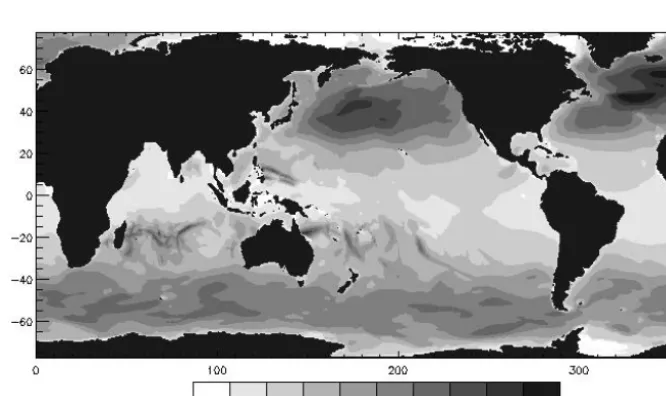
The distribution of annual-average significant wave height provided by the model (Chawla et al., 2013) is shown in
Fig. 2. As seen, the maximum value in the field of annual-average significant wave height does not exceed 5 m (south-ern area of Indian and Pacific oceans), while the height of real extreme waves can reach 16 m in this area. The data in Fig. 1 have a more complicated structure, due, for example, to the periods with strong wind along trajectories of tropi-cal storms. Consequently, the tropi-calculations of the distribution of real wave height should be carried out for shorter periods, i.e. for seasonal or monthly averaged data on significant wave heights.
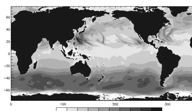
Figure 3 shows the field of wave height above mean level with a probability of 10−7averaged for December–February. When comparing Fig. 3 and Fig. 1 it is seen that in mid-latitudes of the Northern Hemisphere wave heights become higher. In some areas appearance of extreme wave heights exceeding 16 m is possible. At the same time there are actu-ally no extreme waves in the eastern part of the Arctic Ocean, which is connected with seasonal ice formation in the area. In equatorial and tropical areas of the world ocean wave heights are lower in winter (Northern Hemisphere), compared with the average annual wave heights. It should be noted that in the western part of the Atlantic Ocean trajectories of hurri-canes disappeared while the number of such trajectories in-creased in the Indian Ocean.
1324 K. Bulgakov et al.: Evaluation of extreme wave probability on the basis of long-term data analysis
Figure 2.Average annual significant wave height (m).
Figure 3.Wave height above mean level (m) with a cumulative probability of 10−7for December–February.
Summer months (Fig. 5) are characterized by a general de-crease in extreme wave probability. It is especially noticeable in the northern areas of the Atlantic and Pacific oceans. Also, wave heights slightly decreased in the Southern Hemisphere. It should be noted that storm tracks appear off the eastern coast of North America and disappear in the southern part of the Pacific Ocean. In addition, quite distinct trajectories of storms appear in the eastern part of the Pacific Ocean. Small wave heights can be observed in the Arctic Ocean, in the area free from ice.
During autumn months (Fig. 6) an increase in wave heights is observed in the Arctic Ocean, with values of the extreme wave height above mean level sometimes reaching 20 m. Among other features is an increase in the wave-free
area in polar latitudes of the Southern Hemisphere, which is obviously connected with seasonal ice formation.
It is quite evident that the average monthly fields of cumu-lative wave height probability will allow us to obtain more exact information on the areas of extreme wave probability.
4 Discussion and conclusions
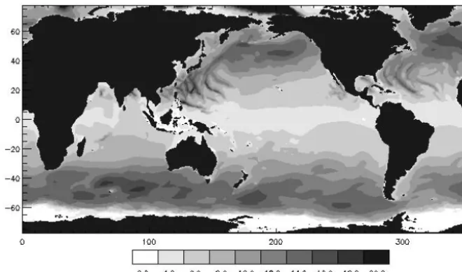
Figure 4.Wave height above mean level (m) with a cumulative probability of 10−7averaged for March–May.
Figure 5.Wave heights above mean level (m) with a cumulative probability of 10−7, for June–August.
The method uses the results of massive numerical simu-lations with 3-D irrotational wave models (Chalikov et al., 2014). Initial conditions for each run were assigned by the JONSWAP spectrum, but for each run random phases were different. Such details of the initial spectrum are not too im-portant. The ensemble modelling is used to eliminate the ef-fects of reversible non-linear interactions causing down shift-ing that can influence the statistics. To be sure that the sim-ulated process can be treated as quasi-stationary; the time of integration was chosen to be relatively short, viz. 350 units of non-dimensional time. The extensive statistics were ob-tained by multiple repetitions of runs with the same initial spectrum. The total number of records used for construction of approximation (Eq. 3) was 4 587 520 000.
1326 K. Bulgakov et al.: Evaluation of extreme wave probability on the basis of long-term data analysis
Figure 6.Wave heights above mean level (m) with a cumulative probability of 10−7, averaged for September–November.
Hence, on the whole, the method considered is suitable for estimation of extreme values of wave heights having small probability.
The maps of the global distribution of wave heights with a probability of 10−7for the main seasons illustrate the ap-proach of the method. Estimation of the return period of a wave with a specific cumulative probability is quite a sophis-ticated problem. It will be the subject of our next work.
We do not state that results of this paper completely solve the problem of treating data on significant wave height in terms of real wave height (above mean level). The most dif-ficult unresolved problem is the problem of estimating con-fidence intervals, which needs further extensive simulation and analysis.
Data availability. Data are available at https://cloud.rshu.ru/index. php/s/5NoHhezK2AEVgzL (Significant wave dataset calculated by WaveWatch III, 2018).
Author contributions. KB conceived the main idea of the article, performed calculation of fields of wave height, and wrote the article. VK and DS carried out visualization of fields.
Competing interests. The authors declare that they have no conflict of interest.
Acknowledgements. The authors are thankful to Dmitry Chalikov for his useful consultations.
The investigation was fulfilled with financial support of the Rus-sian Science Foundation (project no. 16-17-00124).
Edited by: John M. Huthnance Reviewed by: two anonymous referees
References
Bitner-Gregersen, E. M. and Toffoli, A.: On the probability of oc-currence of rogue waves, Nat. Hazards Earth Syst. Sci., 12, 751– 762, https://doi.org/10.5194/nhess-12-751-2012, 2012.
Chalikov, D.: Freak waves: their occurrence and probability, Phys. Fluids, 21, 076602, https://doi.org/10.1063/1.3175713, 2009. Chalikov, D. and Babanin, A. V.: Comparison of linear and
non-linear extreme wave statistics, Acta Oceanol. Sin., 35, 99–105, https://doi.org/10.1007/313131-016-0862-5, 2016.
Chalikov, D. and Bulgakov, K.: Estimation of wave height proba-bility based on the statistics of significant wave height, J. Ocean Eng. Mar. Energy, https://doi.org/10.1007/s40722-017-0093-7, in press, 2017.
Chalikov, D., Babanin, A., and Sanina, E.: Modeling of Three-Dimensional Fully Nonlinear Potential Periodic Waves, Ocean Dynam., 64, 1469–1486, https://doi.org/10.1007/s10236-014-0755-0, 2014.
Chalikov, D. V.: Numerical modeling of sea waves, Springer, Switzerland, 330 pp., 2016.
Chalikov, D. V.: Linear and nonlinear statistics of extreme waves, Russ. J. Numer. Anal. Math. Model., 32, 91–99, 2017.
Chalikov, D. V. and Bulgakov, K. Y.: Numerical modeling of wave development under the action of wind, Phys. Wave Phenom., 25, 315–323, 2017.
Chawla, A., Spindler, D. M., and Tolman, H. L.: Validation of a thirty year wave hindcast using the climate forecast system re-analysis winds, Ocean Model., 70, 189–206, 2013.
Guo, L. and Sheng, J.: Statistical estimation of extreme ocean waves over the eastern Canadian shelf from 30-year numerical wave simulation, Ocean Dynam., 65, 1489–1507, 2015.
Jiangxia, L., Shunqi, P., Yongping, C., Yang-Ming, F., and Yi, P.: Numerical estimation of extreme waves and surges over the northwest Pacific Ocean, Ocean Eng., 153, 225–241, 2018. Kharif, C., Pelinovsky, E., and Slunyaev, A.: Rogue Waves in the
Ocean, in: Advances in geophysical and environmental Mechan-ics and MathematMechan-ics, Springer, Berlin, Germany, 2009. Larsen, X. G., Kalogeri, C., Galanis, G., and Kallos, G.: A
statisti-cal methodology for the estimation of extreme wave conditions for offshore renewable applications, Renewable Energy, 80, 205– 218, 2015.
Ochi, M. K.: Ocean waves: the stochastic approach, in: Cambridge Ocean Technology Series, Cambridge University Press, Cam-bridge, 332 pp., 1998.
Onorato, M., Waseda, T., Toffoli, A., Cavaleri, L., Gramstad, O., Janssen, P. A., Kinoshita, T., Monbaliu, J., Mori, N., Osborne, A. R., Serio, M., Stansberg, C. T., Tamura, H., and Trulsen, K.: Statistical Properties of Directional Ocean Waves: The Role of the Modulational Instability in the For-mation of Extreme Events, Phys. Rev. Lett., 102, 114502, https://doi.org/10.1103/PhysRevLett.102.114502, 2009.
Samayam, S., Laface, V., Annamalaisamy, S. S., Arena, F., Vallam, S., and Gavrilovich, P. V.: Assessment of reliability of extreme wave height prediction models, Nat. Hazards Earth Syst. Sci., 17, 409–421, https://doi.org/10.5194/nhess-17-409-2017, 2017. Sasha, S., Moorthi, S., Pan, H., and Goldberg, M.: The NCEP
cli-mate forecast reanalysis version 2, J. Clicli-mate, 27, 2185–2208, 2014.
Significant wave dataset calculated by WaveWatch III: https://cloud. rshu.ru/index.php/s/5NoHhezK2AEVgzL, last access: 23 Octo-ber 2018.
Tolman, H. L.: User manual and system documentation of WAVEWATCH III version 4.18, Technical Note 316, NOAA/NWS/NCEP/MMAB, College Park, MD, USA, 311 pp., 2014.
Touboul, J. and Kharif, C.: Two-dimensional direct numerical sim-ulations of the dynamics of rogue waves under wind action, Adv. Numer. Simul. Nonlin. Water Waves, 11, 43–74, 2010.