An ensemble-based approach to climate reconstructions

(1)

Clim. Past, 8, 963–976, 2012 www.clim-past.net/8/963/2012/ doi:10.5194/cp-8-963-2012

Climate

of the Past

An ensemble-based approach to climate reconstructions

J. Bhend1,*, J. Franke2, D. Folini1, M. Wild1, and S. Br¨onnimann2

1_{Institute for Atmospheric and Climate Science, ETH Z¨urich, Z¨urich, Switzerland} 2_{Oeschger Centre and Institute of Geography, University of Bern, Bern, Switzerland} *_{now at: CSIRO Marine and Atmospheric Research, Aspendale, Australia}

Correspondence to: J. Bhend ([email protected])

Received: 27 August 2011 – Published in Clim. Past Discuss.: 14 September 2011 Revised: 4 May 2012 – Accepted: 4 May 2012 – Published: 31 May 2012

Abstract. Data assimilation is a promising approach to

tain climate reconstructions that are both consistent with ob-servations of the past and with our understanding of the physics of the climate system as represented in the climate model used. Here, we investigate the use of ensemble square root filtering (EnSRF) – a technique used in weather forecast-ing – for climate reconstructions. We constrain an ensemble of 29 simulations from an atmosphere-only general circula-tion model (GCM) with 37 pseudo-proxy temperature time series. Assimilating spatially sparse information with low temporal resolution (semi-annual) improves the representa-tion of not only temperature, but also other surface proper-ties, such as precipitation and even upper air features such as the intensity of the northern stratospheric polar vortex or the strength of the northern subtropical jet. Given the spar-sity of the assimilated information and the limited size of the ensemble used, a localisation procedure is crucial to reduce “overcorrection” of climate variables far away from the as-similated information.

1 Introduction

Compared to conventional reconstruction methods, data as-similation represents a novel approach to increase our un-derstanding of past climate. In this paper, we explore in an idealised setup if assimilation of sparse and indirect obser-vations of past climate states, as recorded in climate prox-ies, provides sufficient constraints to skilfully update existing model simulations.

Two distinct approaches have often been used when recon-structing past climate: empirical methods relate the changes in climate proxies – such as tree-ring widths or δ18O

concentrations in ice cores – to changes in climate vari-ables during past decades (see Jansen et al., 2007, and Jones et al., 2009, for an overview of recent advances). This lationship is then extended backwards, allowing for the re-construction of said climate variables for times when no di-rect observations of the climate system are available. Em-pirical methods rely on the stationarity of the relationship between climate and proxy record. In addition, the specifics of high-resolution proxy archives make it hard to quantify low-frequency variability (Moberg et al., 2005). Dynamical methods, on the other hand, use reconstructed external forc-ings (e.g. changes in solar irradiance, land cover, atmospheric aerosol and greenhouse gas concentrations) to constrain sim-ulations of past climate states (e.g. Jungclaus et al., 2010; Wanner et al., 2008; Ammann et al., 2007). In contrast to empirical approaches, dynamical methods allow us to also reconstruct climate variables, which are only loosely corre-lated to climate proxies. Ensembles of climate model simula-tions, however, are often not well constrained, as a large part of the variability is generated in the climate system itself and is thus independent of external forcings.

(2)

964 J. Bhend et al.: An ensemble-based approach to climate reconstructions

Additional constraints are therefore needed to solve the prob-lem. These additional constraints originate from the physics and dynamics of the system as formulated in a climate model. The model provides a first guess of the true state of the sys-tem that is consistent with the boundary conditions. This

prior estimate of the true state is updated with observations

to produce the analysis. The model is then used to propa-gate the analysis to provide a first guess for the next analysis cycle. This recursive procedure to accumulate observed in-formation in the model is referred to as data assimilation.

First attempts to assimilate climate proxy information into models include the pioneering work of von Storch et al. (2000), Hargreaves and Annan (2002), van der Schrier and Barkmeijer (2005), Goosse et al. (2006, 2010), and Franke et al. (2010). The proposed approaches can be roughly sepa-rated into three groups: the methods of von Storch et al. and van der Schrier and Barkmeijer seek to push a model simula-tion towards a large-scale target state through nudging (von Storch et al., 2000) or using singular forcing vectors (van der Schrier and Barkmeijer, 2005). The methods by Goosse et al. (2006) and Franke et al. (2010) select optimal matches with the available proxy information among a set of model states and combine these to “pseudo-simulations”. Recently, Goosse et al. (2010) modified their assimilation method to produce dynamically consistent past climate states, based on simulations with an Earth system model of intermediate com-plexity. All of the approaches discussed so far do not gener-ically provide confidence intervals together with their best estimate, a shortcoming that is overcome by the approach proposed by Hargreaves and Annan. In contrast, their fully probabilistic approach is not tractable with a complex and computationally expensive model. Therefore, we propose a new approach that both allows us to assimilate proxy data into a high-resolution general circulation model (GCM) and that provides a generic quantification of the uncertainties.

Data assimilation has long been used in numerical weather forecasting to estimate optimal initial conditions for weather predictions (Kalnay, 2003). The variational data assimilation techniques developed for weather forecasting, however, are not suitable for reconstruction of past climate with a much smaller number of observations or climate proxies. A much simpler to implement and computationally less expensive method to assimilate data into climate model simulations is represented by the class of square root filters.

We use the ensemble square root filter (EnSRF) – a vari-ant of the ensemble Kalman filter (EnKF; see Evensen, 2003, and references therein) – as introduced by Whitaker and Hamill (2002) to update the ensemble of model simulations with information from climate proxies. The EnSRF has suc-cessfully been used to produce a reanalysis for the period from 1870 to present using sea level pressure measurements (Compo et al., 2006, 2011). Here, we investigate whether En-SRF can also be used with spatially sparse observations with low temporal resolution.

Our main goal is to learn to what extent and under what conditions proxy data provide sufficient constraints for a data assimilation approach to climate reconstructions using the EnSRF algorithm. For this introductory analysis, we use a perfect model framework to explore the potential benefits of an ensemble-based approach to climate reconstructions. One simulation of the ensemble describes the true climate from which we generate pseudo-proxies, and the remaining simu-lations are used to estimate the true climate.

To be able to experiment with the details of the setup and properly explore the potential of an ensemble-based ap-proach to reconstructions at a reasonable computational cost, we want to be able to run the assimilation off-line. Thus, we use an atmosphere-only GCM to describe past climates. In this setup, the proxy information has a temporal resolution (semi-annual in our case) that is far greater than the determin-istic predictability of most atmospheric processes (Lorenz, 1969; Kalnay, 2003). This discrepancy in time scales be-tween the memory of the system (a few days) and the obser-vation interval (semi-annual) has profound implications for the proposed assimilation approach.

In a conventional assimilation, the effect of constraining the model with past observations gets propagated by the model and determines to a large extent the current first guess (unconstrained simulation). This is not the case in our ide-alised setup. Due to the chaotic nature of the atmosphere, the effect of the previous update (leading to the new analysis) is lost long before the end of the simulation cycle. That is, a forward integration of a constrained simulation and an un-constrained simulation are indistinguishable after six months on average. Thus, observed information does not accumu-late over time, but only current observed information con-strains the model. Therefore, we can assimilate the data non-recursively; that is, we do not need to feed back the corrected states (the analysis) as new initial conditions for the next sim-ulation cycle. Consequently, we should not refer to the ap-proach as a filter. Instead, we suggest to refer to the method as ensemble square root fitting.

Ultimately, we aim at assimilating climate proxy data into a coupled atmosphere-ocean GCM. In such a coupled sys-tem, there is far more long-term memory, and thus we will need to revert to the conventional recursive assimilation pro-cedure. In the light of the final goal and to highlight the ori-gins of the approach, we do not resolve the ambiguity in the abbreviation and we keep referring to our simplified ap-proach as EnSRF.

(3)

J. Bhend et al.: An ensemble-based approach to climate reconstructions 965

2 Materials and analysis metrics

2.1 Model simulations

For the assessment of EnSRF for climate reconstructions, we used an initial condition ensemble of 30 simulations with the general circulation model (GCM), ECHAM5.4 (Roeck-ner et al., 2003, 2004). The model was run in T63L31 resolu-tion, corresponding to an approximate horizontal resolution of 1.875◦with 31 vertical levels from the surface to 10 hPa.

ECHAM5.4 was forced with reconstructed sea surface temperatures (SST, reconstruction by Mann et al., 2009), augmented with ENSO-dependent intra-annual variability according to the reconstructed NINO3.4 index of Cook et al. (2008) and climatological sea-ice according to the HadISST climatology (Rayner et al., 2003). We further used recon-structed solar irradiance (Lean, 2000) and land surface pa-rameters derived from the land-use reconstructions of Pon-gratz et al. (2008). Additionally, the model was forced with reconstructions of volcanic activity by Crowley et al. (2008) and concentrations of long-lived greenhouse gases as used in Yoshimori et al. (2010, and references therein). Finally, tran-sient sulphate concentrations were prescribed according to the reconstructed aerosol loads of Koch et al. (1999); before 1850, tropospheric sulphate aerosol concentrations were set to their 1850 values.

The solar irradiance reconstruction by Lean (2000) ex-hibits an increase in irradiance of approximately 2.5 W m−2 since the Maunder Minimum (MM). Recent reconstructions, however, show less of a change in solar irradiance between the MM and present conditions (Wang et al., 2005; Krivova et al., 2007). Nevertheless, we chose a strong solar forcing, as the recent study by Jungclaus et al. (2010) has shown that this leads to a slightly more realistic climate response over the past 1000 yr in ECHAM5.4.

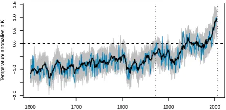
The individual simulations were branched off from a con-trol run reflecting conditions around 1600 AD. The boundary conditions for the atmospheric model were prescribed and identical across the thirty different ensemble members. The spread of the initial condition ensemble thus reflects inter-nal variability of the atmosphere alone. The time series of Northern Hemispheric annual average temperatures north of 20◦N (in Fig. 1) illustrate the relative importance of exter-nal forcings and interexter-nal variability. The forced response of 2◦C warming from 1600 to 2000 in the extratropical North-ern Hemisphere is slightly stronger than previous coupled AOGCM simulations (Gonz´alez-Rouco et al., 2003; Am-mann et al., 2007; Tett et al., 2007; Jungclaus et al., 2010). Relative to the forced response, the annual internal variabil-ity is pronounced even in this atmosphere-only simulation, indicating the potential for constraining the ensemble with additional information.

We analyse simulated near-surface temperature and pre-cipitation over land and several derived indices characteris-ing atmospheric circulation accordcharacteris-ing to Br¨onnimann et al.

12 J. Bhend et al.: An ensemble-based approach to climate reconstructions

1600 1700 1800 1900 2000

−2.0

−1.0

0.0

0.5

1.0

1.5

T

emper

ature anomalies in K

Fig. 1.Annual (November to October) average temperature north of 20◦_{N in the ensemble of ECHAM5.4 simulations as anomalies}

of the 1961-90 mean. The grey area denotes the range of the first 29 individual simulations, the thick black line is the corresponding ensemble average and the thin blue line denotes the thirtieth simu-lation (the reference).

Fig. 1. Annual (November to October) average temperature north of 20◦N in the ensemble of ECHAM5.4 simulations as anomalies of the 1961–1990 mean. The grey area denotes the range of the first 29 individual simulations; the thick black line is the corresponding ensemble average and the thin blue line denotes the 30th simulation (the reference).

(2009). The data are aggregated for boreal winter (Novem-ber to April) and summer (May to Octo(Novem-ber), reflecting the approximate temporal resolution of climate proxies. In order to keep computations tractable, we thinn out the initial model grid by selecting grid boxes only at every third longitude and latitude. The state vector used in the EnSRF approach thus consists of semi-annual temperature and precipitation at 694 locations over land plus four derived indices. These indices include the strength of the northern subtropical jet (SJ), de-fined as the maximum zonal-mean zonal wind at 200 hPa be-tween the Equator and 50◦_{N, the strength of the Hadley cell}

(HC), defined as the maximum of the zonal mean meridional stream function at 500 hPa between the Equator and 30◦N, the strength of the northern stratospheric polar vortex (z100), defined as the difference in geopotential height at 100 hPa between 75–90◦N and 40–55◦N, and the dynamic Indian monsoon index (DIMI), defined as the difference in average zonal winds at 850 hPa in the boxes 5–15◦N, 40–80◦E and 20–30◦N, 70–90◦E. For further discussion of these indices, please refer to Br¨onnimann et al. (2009).

From the 405-yr period of simulations from 1601 to 2005, we select the segment of 135 yr from 1871 to 2005 for the analysis. For this period, the simulations were constrained with observed rather than reconstructed SSTs and sea-ice variability as boundary conditions. The spatio-temporal vari-ability of reconstructed SSTs is considerably different from variability in observed SSTs. The results, however, are qual-itatively robust to results obtained when assimilating proxy data in the early part of the simulation (not shown).

2.2 Pseudo-proxy generation

(4)

different locations (see Fig. 2). The pseudo-proxy locations are chosen to reflect the distribution of temperature-sensitive proxies over land, such as tree-ring series and ice cores (e.g. Mann et al., 2009). Proxy networks such as collections of tree-ring series in North America and Europe are represented by a single pseudo-proxy.

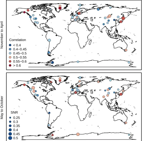
We use a simple approach to fabricate pseudo-proxy time series following earlier work (Mann and Rutherford, 2002; von Storch et al., 2009): at each proxy location, we add nor-mally distributed white noise to the temperature time series of the reference simulation. The noise variance is scaled to produce signal-to-noise ratios of 0.33 or correlations of 0.5 on average. Due to the limited sample size, the actual corre-lations range from 0.36 to 0.66 and the signal-to-noise ratio from 0.26 to 0.46, as shown in Fig. 2. The pseudo-proxies are also slightly biased compared to the original series, with normally distributed biases centred at zero and ranging from −0.4 to 0.5 K (not shown). The bias in the pseudo-proxy time series reflects a potential estimation error when calibrating real-world proxy time series. Unlike a real-world situation, however, the noise added to the reference time series does not exhibit spatio-temporal coherence.

2.3 Metrics of skill and reliability

We analyse the skill in reconstructing different global and continental-scale indicators. Skill is measured using a mean squared error skill score (Murphy and Epstein, 1989), which is also known as the reduction of error (RE, Cook et al., 1994):

RE=1−

P

(x_ia−x_iref)2 P

(x_ib−x_iref)2 (1)

xa andxb denote the analysis and the unconstrained initial condition simulation, respectively;xrefis the reference sim-ulation (the target). The summation is overi, andi counts the different time steps. This skill score ranges from 1 to −∞; positive values indicate that the analysis is closer to the reference simulation in mean square error terms than the unconstrained simulation. As we constrain the full set of sim-ulations, we investigate both the skill score for the ensemble mean and the individual simulations. In doing so, we com-pare the ensemble mean analysisx¯awith the unconstrained ensemble meanx¯b, and each individual analysis simulation with its unconstrained counterpart.

Furthermore, we also analyse the change in correlation from the correlation of the unconstrained simulations with the reference simulation to the correlation of the analysis with the reference simulation.

Our method for reconstructing past climate states produces not only a best estimate of the past climate state, but also an associated uncertainty estimate. To assess whether the un-certainty is correctly reflected in the ensemble-based, proba-bilistic prediction (the analysis), the concept of reliability is

J. Bhend et al.: An ensemble-based approach to climate reconstructions 13

No

v

ember to Apr

il ● ● ● ● ● ●● ● ● ● ● ● ● ● ● ● ● ● ● ● ● ● ● ● ● ● ● ● ●● ● ● ● ● ● ● ● ● ● ● ● ● ● Correlation < 0.4 0.4−0.45 0.45−0.5 0.5−0.55 0.55−0.6 > 0.6 Ma

y to October

● ● ● ● ● ● ● ● ● ● ● ● ● ● ● ● ● ● ● ● ● ● ● ● ● ● ● ● ● ● ● ● ● ● ● ● ● ● ● ● ● ● ● SNR 0.25 0.3 0.35 0.4 0.45 0.5

Fig. 2.Correlation and signal-to-noise ratio of pseudo-proxies with reference time series in boreal winter (November to April, upper panel) and summer (May to October, lower panel). The colour in both panels reflects the correlation according to the legend in the upper panel, the size of the circles in both panels reflects the signal-to-noise ratio according to the legend in the lower panel.

Fig. 2. Correlation and signal-to-noise ratio of pseudo-proxies with reference time series in boreal winter (November to April, upper panel) and summer (May to October, lower panel). The colour in both panels reflects the correlation according to the legend in the upper panel; the size of the circles in both panels reflects the signal-to-noise ratio according to the legend in the lower panel.

employed. A probabilistic prediction system is deemed re-liable if the frequency of occurrence matches the predicted probability over a large set of predictions. For ensemble-based systems, the analysis rank histogram allows us to as-sess the reliability of the prediction system (Anderson, 1996). The rank histogram is produced by computing the rank of the observations of the true climate state (here the ref-erence simulation) compared with the sorted ensemble of predictions (the analysis) for each individual grid box and time step. In a perfectly reliable ensemble, we would expect the observations to fall in each of thenens+1 classes with equal probability, thus resulting in a flat rank histogram. A U-shaped histogram, in contrast, indicates a negative bias in the analysis variance, i.e. the ensemble is overconfident and the true climate state often lies outside the range of values predicted by the analysis. Correspondingly, a dome-shaped rank histogram denotes an analysis ensemble that overem-phasises uncertainty.

(5)

3 Ensemble Square Root Fitting

We use a variant of ensemble Kalman filtering (EnKF, see Evensen, 2003, and references therein) to update model sim-ulations with measurements of the climate system – here pseudo-proxy time series derived from one model simu-lation. For readers not familiar with EnKF, we provide a short introduction before discussing the modifications and specifics of the approach used in this study. For a more com-prehensive introduction, please refer to the above reference.

Data assimilation seeks to provide a best estimate of the true climate state – the analysis. As the problem is not well constrained by the often sparse observations, additional con-straints from mathematical models are used to estimate the analysis. Specifically, the models are used to provide a first guess of the true climate state consistent with the boundary conditions. This prior estimate of the background climate is then updated with the observations to form the posterior dis-tribution of the analysis. The data assimilation can thus be expressed as a Bayesian update problem with

P (xa|y)∼P (y|xb) P (xb). (2)

WhereP (∗|∗)denotes a conditional probability,xis the cli-mate state in the model andy contains the observations of the climate state. For clarification, the background or prior distribution of the climate state is indicated with the super-script “b” as inxb_{, and the analysis or posterior is denoted} with superscript “a”. In addition to providing a first guess of the true climate state, the mathematical model is also used to propagate the analysis for providing a first guess for the next analysis cycle if the data assimilation procedure is cy-cled. Thereby, the analysis is consistent with all previous and current observations. As discussed earlier, we do not use a cycling of the procedure and therefore, the analysis is con-strained by current observations only. In the linear Gaussian case, the above Bayesian update is identical with the Kalman filter update.

In the Gaussian case, we can characterise the background climate at a given time through its meanx¯band its covariance matrix Pb, wherex¯bis a vector of lengthn, the dimension of the model state, and Pbis a matrix of dimensionn×n. The observations y of the true state are collected at mdistinct points, withmnin general. We account for the fact that

y consists of indirect observations of the true state and as-sume the observation error to follow a zero-mean Gaussian process with covariance R, the observation error covariance. To link model and observation space, we define the operator

H of dimensionm×nthat extracts the observations from the

model space. H can be non-trivial in a paleoclimatology con-text, as this operator reflects the complex dependence of cli-mate proxies, such as tree rings on clicli-mate. In our idealised study, however, H only extracts temperature at proxy loca-tions from the model statex¯b. The development of proxy for-ward models and corresponding observation operators will be dealt with elsewhere.

The analysis in Kalman filtering is again a multivariate Gaussian, with meanx¯aand covariance Pa. Following the no-tation in Whitaker and Hamill (2002), the traditional Kalman filter update equations for the mean and covariance are

¯

xa=x¯b+K(y−Hx¯b) (3)

Pa=(I−K H)Pb (4)

K=PbHT(HPbHT +R)−1 (5)

K denotes the Kalman gain, a matrix of dimensionn×m,

and I is then×nidentity matrix.

In the ensemble Kalman filter (EnKF), the mean states and covariances are approximated by the sample mean and co-variance based on a finite number of simulations. Thus, the background mean in EnKF isx¯b=1/nensP_kxb_k, where k counts the nens ensemble members used. Correspondingly, the background covariance is Pb=1/(nens−1)P_k(xb_k−

¯

xb)2. Given that the true mean states and covariances are never known, but estimated, the ensemble approximation is an intuitive and more practically relevant representation of the problem than the general case. Hereafter, mean statesx¯, covariances P, and the corresponding Kalman gain K denote the sample-based EnKF representation of these quantities.

In addition to being of more practical relevance than the Kalman filter, the EnKF also allows us to express the fil-tering problem in a computationally more efficient way. In-stead of operating on the full n×n covariance matrix, the ensemble members are updated individually without explic-itly updating the covariances. To reflect the observation error distribution, the observations used to update each individual simulation have to be randomly perturbed according to the observation error covariance. Consequently, EnKF is biased due to sampling uncertainty in both the background covari-ance Pb estimated from the ensemble of model simulations and the observation perturbations. Due to the nonlinear de-pendence of the analysis covariance Pa on the background covariance Pb, Pa will be biased low and therefore under-estimate ensemble mean errors on average. This underesti-mate of Pa can lead to filter divergence and will result in an overly confident analysis in general. The perturbation of observations also increases sampling error and leads to the analysis-error covariance estimate Pabeing less accurate on average. To overcome the above limitations, Whitaker and Hamill (2002) propose a novel approach that does not rely on the perturbation of observations; this approach is referred to as the ensemble square root filter (EnSRF).

Using EnSRF, the update is separated into an ensemble mean update (Eq. 6), which is identical to the EnKF update and an update of the anomalies about the ensemble mean (Eq. 7; see Whitaker and Hamill 2002). Thus, we decompose the background statexbinto the ensemble mean background statex¯b_{and the deviation from the ensemble mean}_x0b

(6)

¯

xa=x¯b+K(y¯−Hx¯b) (6)

x0a=x0b+ ˜K(y0−Hx0b)=(I− ˜KH)x0bwith:y0=0 (7) The Kalman gain matrix K is identical to the gain matrix in the classical EnKF approach as shown in Eq. 5. The gain matrix for the ensemble anomalies,K, is expressed as fol-˜

lows: ˜

K=PbHT

p

HPb_HT₊_R−1

T

×

p

HPb_HT₊_R₊√_R−1 ₍₈₎

In our implementation, the background statexb is a vec-tor of length n= 1392, consisting of semi-annual tempera-ture and precipitation over land at 694 grid boxes and 4 de-rived indices. We assimilate pseudo-proxies atm= 37 loca-tions. As the pseudo-proxies are generated from the true cli-mate state (the reference simulation) by adding white noise, the observation error variances are known and the covariance matrix R is diagonal. Therefore, we can update the ensemble serially by including one observation at a time. This greatly enhances the computational tractability of the problem.

3.1 Ensemble covariance localisation

Simulating large ensembles of high-resolution GCMs is ex-pensive. Consequently, we have to estimate the background error covariance from a rather limited set of simulations. Here, we estimate the 1392×1392 dimensional background error covariance matrix Pbfrom an ensemble of only 29 sim-ulations. The use of a finite ensemble to approximate the background error covariance leads to spurious correlations off the diagonal in Pb. These spurious correlations result in small unphysical updates and reduce the analysis variance. In the recursive implementation, this effect will lead to filter di-vergence. In our non-recursive implementation, the sampling uncertainty leads to an overly confident reconstruction.

Various approaches exist to correct for spurious correla-tions in the background error covariance and to thereby avoid filter divergence. Covariance inflation (Anderson and An-derson, 1999) and covariance localisation (Houtekamer and Mitchell, 2001) are two commonly used strategies. The for-mer compensates for filter divergence by inflating the back-ground error covariance previous to the update step. The lat-ter is based on the assumption that the correlation between variables decreases with distance between the variables. In this study, we apply a simple covariance localisation to deal with spurious correlations. The localisation reflects our be-lief that the analysis at each grid box depends more strongly on observed information that is close by than on very distant observations.

To ensure that the localised background error covariance is positive-definite, we use an element-wise product of the sam-ple covariance and a correlation function with local support (see Gaspari and Cohn, 1999, for correlation functions). We redefine Pb used in the EnSRF algorithm above to account for spurious correlations according to Eq. 9:

p_i,jb = 1

nens−1 nens X

k=1

x0b_i,kx0b_j,k exp −|di−dj| 2

2L2 !

(9)

p_i,jb denotes row numberi and column numberj of Pb; k

indexes thenensdifferent ensemble members.|di−dj|is the

distance in km between grid boxiand grid boxj, andLis the cutoff distance at which the sample covariance decreases by 39 %. For the aggregated indices in the state vector,|di−dj|

is set to the minimum distance between the respective grid boxiand the points in the box used to compute the index cor-responding toj (or vice versa). The influence of the choice ofLon the analysis is discussed in the following.

4 Results

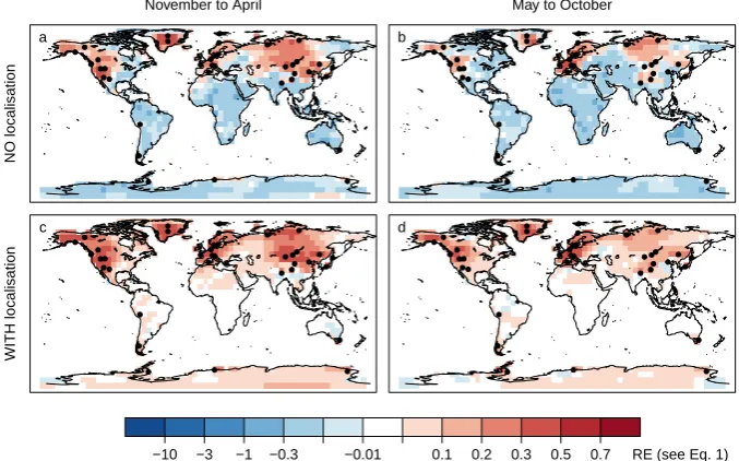
First, we analyse the effect of the covariance localisation to deal with spurious covariances. Figure 3 illustrates the benefits of localisation of Pb. Without localisation, skill – measured in terms of mean squared error of the ensemble mean compared with the reference time series (see Eq. 1) – is confined to the regions where proxy data are assimilated; elsewhere, we find negative skill. That is, without localisa-tion, assimilation of pseudo-proxies leads to an “overcorrec-tion” of the ensemble in regions far away from where in-formation is assimilated (Fig. 3a and b). With localisation, skill is less confined to the regions where we assimilate data (Fig. 3c and d), as the closest proxies are given more weight in the data assimilation procedure. For example, we find pos-itive skill almost throughout North America with localisa-tion, whereas without localisalocalisa-tion, positive skill is confined to western North America, where proxy information is as-similated. In regions far away from proxy locations, such as Africa or the Amazon Basin, the above mentioned overcor-rection disappears, resulting in zero skill.

(7)

J. Bhend et al.: An ensemble-based approach to climate reconstructions 969 14 J. Bhend et al.: An ensemble-based approach to climate reconstructions

November to April

NO localisation ● ● ● ● ● ● ● ● ● ● ● ● ● ● ● ● ● ● ● ● ● ● ● ● ● ● ● ● ● ● ● ● ● ● ● ● ● a

May to October

● ● ● ● ● ● ● ● ● ● ● ● ● ● ● ● ● ● ● ● ● ● ● ● ● ● ● ● ● ● ● ● ● ● ● ● ● b WITH localisation ● ● ● ● ● ● ●● ● ● ● ● ● ● ● ● ● ● ● ● ● ● ● ● ● ● ● ● ● ● ● ● ● ● ● ● ● c ● ● ● ● ● ● ●● ● ● ● ● ● ● ● ● ● ● ● ● ● ● ● ● ● ● ● ● ● ● ● ● ● ● ● ● ● d

−10 −3 −1 −0.3 −0.01 0.1 0.2 0.3 0.5 0.7 RE (see Eq. 1)

Fig. 3.Mean square error skill score (RE) for near-surface temper-ature of the analysis ensemble mean compared to the unconstrained ensemble mean without (panels a and b) and with localisation (c and d). Results for boreal winter (November to April, a and c) and for boreal summer (May to October, b and d). Black dots indicate locations at which pseudo-proxies are assimilated.

Fig. 3. Mean square error skill score (RE) for near-surface temperature of the analysis ensemble mean compared to the unconstrained ensemble mean without (a and b) and with localisation (c and d). Results for boreal winter (November to April, a and c) and for boreal summer (May to October, b and d). Black dots indicate locations at which pseudo-proxies are assimilated.

the cross-validation with the unconstrained ensemble (black lines in Fig. 4), deviations from a flat rank histogram are in-distinguishable from the rank histogram of a perfectly reli-able ensemble for cutoff lengths of 2000 km and less. There-fore, we set the cutoff length at 2000 km for all further anal-yses.

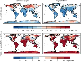
While covariance localisation reduces the negative impact of spurious correlations on the analysis variance, it also af-fects the sharpness of the analysis. The spread of the ensem-ble – here expressed as the intra-ensemensem-ble standard deviation – indicates the sharpness of the hindcast. In the case of the unconstrained hindcast, the spread represents the uncertainty due to internal variability. In the case of the analysis, we hope to make use of the information about the state of internal variability of the reference, and thus we expect to reduce the hindcast uncertainty, and thereby reduce ensemble spread. The influence of the data assimilation on the ensemble spread for temperature is shown in Fig. 5. The ensemble spread, and thus the uncertainty in the hindcast, is significantly reduced in regions close to the assimilated information (Europe, Cen-tral Asia and western North America). As a consequence of the localisation, the spread is not reduced in regions far from the assimilated information (e.g. Sub-Saharan Africa). In ad-dition, data assimilation leads to more wide-spread and larger reductions in ensemble spread in boreal winter than in boreal summer.

In the following figures, the skill scores (Eq. 1) for the re-spective ensemble means are displayed as arrowheads and the individual simulations as box plots (see Fig. 6). The boxes indicate the interquartile range of the 29 simula-tions in the analysis; the thick horizontal line indicates the

median simulation, and the whiskers denote the range of the simulations.

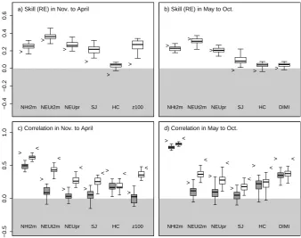
In Fig. 6, Northern Hemispheric and northern European land temperature, northern European precipitation, and var-ious circulation indices are analysed in detail. These aggre-gated indices have been chosen to illustrate the advantages and limitations of the method. We analyse both the mean square error skill score (Eq. 1, Fig. 6a and b) and changes in correlation (Fig. 6c and d) between the unconstrained en-semble and the analysis. The skill score is generally slightly more positive for the individual simulations (boxes in Fig. 6, a and b) than for the ensemble average (arrowheads in Fig. 6). This is due to the fact that the unconstrained ensemble aver-age is – due to its low variance and small bias – an a priori good guess for an additional simulation in mean square error terms. Correlation of the ensemble mean with the reference simulation, however, is generally greatly increased when in-formation is assimilated (see Fig. 6c and d).

(8)

J. Bhend et al.: An ensemble-based approach to climate reconstructions 15

0 5 11 18 25 a) no localisation

0 5 11 18 25 b) L = 5000 km

0 5 11 18 25 c) L = 2000 km

0 5 11 18 25 d) L = 1000 km

Fig. 4. Rank histogram of the reference simulation compared to the analysis using different lengths for the covariance localisa-tion. Without covariance localisation, the spread of the ensemble is negatively biased leading to a strongly U-shaped rank histogram. The black lines are empirical confidence intervals from a cross-validation with the unconstrained ensemble using each of the 30 simulations as observations in turn (see text for further discussion). The red line indicates the rank histogram of the reference simula-tion against the unconstrained ensemble. The scale on the y-axis is the same for all plots and the frequency of occurrence of ranks 0 and 29 are clipped in panel a).

Fig. 4. Rank histogram of the reference simulation compared to the analysis using different lengths for the covariance localisation. Without covariance localisation, the spread of the ensemble is negatively biased, leading to a strongly U-shaped rank histogram. The black lines are empirical confidence intervals from a cross-validation with the unconstrained ensemble, using each of the 30 simulations as observations in turn (see text for further discussion). The red line indicates the rank histogram of the reference simulation against the unconstrained ensemble. The scale on the y-axis is the same for all plots, and the frequency of occurrence of ranks 0 and 29 are clipped in (a).

16 J. Bhend et al.: An ensemble-based approach to climate reconstructions

November to April

Ensemb

le spread

a

May to October

b

0.2 0.4 0.6 0.8 1 1.2 1.4 1.6 1.8 2 2.2 in units of K

Fr

action of spread after assimilation

●

● ●

●

● ●

●

● ●

● ● ●

● ●

● ● ●

● ●

●

● ●

●

● ●

● c

●

● ●

●

● ●

●

● ●

● ● ●

● ●

● ● ●

● ●

●

● ●

●

● ●

● d

25 50 70 80 85 90 94 97 in percent

Fig. 5.Average intra-ensemble standard deviation (spread) for tem-perature of the ECHAM ensemble in winter (a, November to April) and summer (b, May to October). Percentage of the intra-ensemble standard deviation in the analysis ensemble with respect to the un-constrained ensemble for the EnSRF analysis with pseudo-proxies and localisation in c and d.

Fig. 5. Average intra-ensemble standard deviation (spread) for temperature of the ECHAM ensemble in winter (a, November to April) and summer (b, May to October). Percentage of the intra-ensemble standard deviation in the analysis ensemble with respect to the unconstrained ensemble for the EnSRF analysis with pseudo-proxies and localisation in (c) and (d).

Correlation increases considerably with data assimilation for all indicators except HC and DIMI (Fig. 6c). For north-ern European temperature over land (NEUt2m), correlation of most individual simulations (boxes) increases from close to zero to around 0.5 after assimilation. As with skill, the ben-efits of data assimilation decrease with increasing distance from the assimilated information. In boreal summer, in con-trast, increases in correlation after data assimilation are much more moderate (Fig. 6d).

To test the robustness of the results to the choice of ref-erence simulation, we performed a cross-validation using each individual simulation as reference in turn. Although the choice of reference simulation leads to slight differences in the results, the findings presented here are qualitatively ro-bust to the choice of reference simulation (not shown).

(9)

J. Bhend et al.: An ensemble-based approach to climate reconstructions 971 J. Bhend et al.: An ensemble-based approach to climate reconstructions 17

−0.4

−0.2

0.0

0.2

0.4

0.6

> >

>

> >

NHt2m NEUt2m NEUpr SJ HC z100

a) Skill (RE) in Nov. to April

> >

>

> > >

NHt2m NEUt2m NEUpr SJ HC DIMI

b) Skill (RE) in May to Oct.

−0.5

0.0

0.5

1.0

>

> > >

> <

<

< < <

NHt2m NEUt2m NEUpr SJ HC z100

c) Correlation in Nov. to April

>

> >

> <

< _<

< <

<

NHt2m NEUt2m NEUpr SJ HC DIMI

d) Correlation in May to Oct.

Fig. 6. Mean square error skill score (see Eq. 1) for boreal win-ter and summer in panels a and b, and correlation for boreal winwin-ter and summer in panels c and d respectively for seven large-scale indicators. The indicators are: northern hemispheric near-surface temperature over land (NHt2m), northern European temperature (NEUt2m) and precipitation (NEUpr) over land, the strength of the northern subtropical jet (SJ), the northern Hadley cell (HC), the stratospheric polar vortex (z100, boreal winter only), and the dy-namic Indian monsoon index (DIMI, boreal summer only). Boxes indicate the interquartile range of skill scores (correlation) for the individual simulations and the whiskers indicate the range of skill scores(correlation), the arrowheads indicate the skill scores (corre-lation) of the ensemble mean. In panels c and d, the grey boxes and right-facing arrowheads indicate correlation between the un-constrained ensemble and the reference simulation, the white boxes and left-facing arrowheads are the correlation between the simula-tions after data assimilation and the reference simulation.

Fig. 6. Mean square error skill score (see Eq. 1) for boreal winter and summer in (a) and (b), and correlation for boreal winter and summer in (c) and (d) respectively for seven large-scale indicators. The indicators are Northern Hemispheric near-surface temperature over land (NHt2m), northern European temperature (NEUt2m) and precipitation (NEUpr) over land, the strength of the northern subtropical jet (SJ), the northern Hadley cell (HC), the stratospheric polar vortex (z100, boreal winter only), and the dynamic Indian monsoon index (DIMI, boreal summer only). Boxes indicate the interquartile range of skill scores (correlation) for the individual simulations, and the whiskers indicate the range of skill scores(correlation); the arrowheads indicate the skill scores (correlation) of the ensemble mean. In (c) and (d), the grey boxes and right-facing arrowheads indicate correlation between the unconstrained ensemble and the reference simulation; the white boxes and left-facing arrowheads are the correlation between the simulations after data assimilation and the reference simulation.

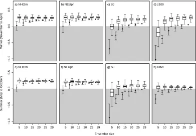
estimated directly from the ensemble. Thus, increasing en-semble size allows us to capture more details of the interrela-tion of variables and its spatial features. In addiinterrela-tion, estima-tion errors decrease with increasing ensemble size. Compu-tation of very large ensembles, however, is very costly, and therefore we would like to learn about minimal requirements for climate reconstructions. Therefore, we run the EnSRF ap-proach with randomly selected sets of 5, 10, 15, 20, 25, and 29 ensemble members and compare the results with the ref-erence simulation. In order to reduce sampling issues, we re-peated the experiment 10 times for each ensemble size.

Mean square error skill generally increases with ensem-ble size for the various indicators (shown in Fig. 7). This increase in skill is moderate for indicators close to the as-similated information, such as mean temperature over land in the Northern Hemisphere or northern European total pre-cipitation (Fig. 7a, b, e and f). In contrast, the increase in skill with increasing ensemble size is considerable for indi-cators further away from the assimilated information, such as the strength of the subtropical jet (SJ, Fig. 7c and g) or the strength of the stratospheric polar vortex (z100, Fig. 7d). For these indicators, we find positive skill for most of the

individual simulations only with ensembles of size 10 or more. We find simulations that perform well even with small ensembles; the positive effect of increasing ensemble size, however, is clearly visible in reducing the number of simula-tions with negative skill. For indicators with marginal skill, such as the dynamic Indian monsoon index (DIMI, Fig. 7h), increasing ensemble size reduces the spread in the results for the individual simulations without affecting the overall skill. For all indicators, the ensemble mean skill strongly benefits from large ensembles.

5 Discussion

(10)

972 J. Bhend et al.: An ensemble-based approach to climate reconstructions 18 J. Bhend et al.: An ensemble-based approach to climate reconstructions

a) NHt2m

−1.0

−0.5

0.0

0.5

Winter (No

v

ember to Apr

il)

b) NEUpr c) SJ d) z100

e) NHt2m

−1.0

−0.5

0.0

0.5

Summer (Ma

y to October)

5 10 15 20 25 29

f) NEUpr

5 10 15 20 25 29 g) SJ

5 10 15 20 25 29

h) DIMI

5 10 15 20 25 29

Ensemble size

Fig. 7. Skill in dependence of ensemble size for different aggre-gated indicators. The boxes summarise the distribution of the mean squared error skill for individual simulations (10 times the number of ensemble members). The black bars denote the spread of skill for the ensemble mean for the 10 different realisations of varying ensemble size, the black diamond indicates the average ensemble mean skill over these 10 realisations. For 29 ensemble members, there is only one analysis.

Fig. 7. Skill in dependence of ensemble size for different aggregated indicators. The boxes summarise the distribution of the mean squared error skill for individual simulations (10 times the number of ensemble members). The black bars denote the spread of skill for the ensemble mean for the 10 different realisations of varying ensemble size; the black diamond indicates the average ensemble mean skill over these 10 realisations. For 29 ensemble members, there is only one analysis.

northern subtropical jet or the strength of the polar vortex through assimilation of surface quantities (here indirect and thus noisy observations of near-surface temperature).

Skill is generally confined to the Northern Hemisphere. This is a consequence of both the greater number of proxy records and the larger fractional land area in the Northern Hemisphere. As a consequence of the experimental setup (an atmosphere-only GCM), we do not expect large differences over oceans and adjacent land due to the dominant influence of sea surface temperatures (SSTs), which are prescribed in the model simulations. We find strongest positive skill for variables in boreal winter, during which weather in the north-ern midlatitudes is strongly influenced by large-scale circu-lation. In boreal summer, when weather is much more de-pendent on local processes, data assimilation is less bene-ficial (see Fig. 6). This finding is in line with other studies (Br¨onnimann and Luterbacher, 2004; Rutherford et al., 2005; Franke et al., 2010; Griesser et al., 2010).

We assimilate semi-annual data and analyse skill both in summer and in winter. The extension of the methodology to be able to assimilate data with higher (monthly) or lower (an-nual to decadal) temporal resolution is straightforward. Most temperatusensitive climate proxies, such as tree rings, re-flect summer temperatures; however, we assess skill also for the winter half-year in order to explore the potential benefits

of assimilating early instrumental observations and docu-mentary evidence.

The skill metric presented here reflects value added to the initial condition ensemble by the data assimilation. The re-sults are thus not comparable with previous studies mak-ing use of pseudo-proxies (Mann and Rutherford, 2002; von Storch et al., 2004; B¨urger et al., 2006). In the following, we highlight the most important difference between the study presented here and earlier work involving pseudo-proxies. The crucial element of empirical climate reconstructions is to establish the relationship between proxy records and cer-tain climatic features (e.g. local climate or large-scale pat-terns) in the calibration period. Pseudo-proxy analyses have been used to investigate how well these relationships can be extrapolated to characterise past climates (see Rutherford et al., 2005; B¨urger et al., 2006; Mann et al., 2007; Chris-tiansen et al., 2009, for a discussion of different reconstruc-tion methods). In the data assimilareconstruc-tion framework, the proxy-climate relationship is characterised by the observation op-erator H and the update of the unconstrained model simu-lations further depends on the observation error covariance

R and the background error covariance Pb. As we are

(11)

R. Instead, we focus on the differences between an

uncon-strained ensemble and the analysis after data assimilation. Nevertheless, we recognise that correct formulation of for-ward proxy models and their related observation operators is crucial for real-world applications of the data assimilation procedure for climate reconstruction, and we are currently working on this issue.

Correlations between individual simulations and the ref-erence simulation improve considerably after assimilation of pseudo-proxies (Fig. 6c and d). This indicates that we can indeed use data assimilation to constrain internal variability. It is noteworthy that positive correlations occur also in the unconstrained simulations (grey boxes and right-facing ar-rows), indicating that the individual ensemble members co-vary with the reference simulation. This is due to the de-terministic response to changing boundary conditions, as il-lustrated for annual average temperature north of 20◦_{N in}

Fig. 1. Due to the strong anthropogenic forcing during the twentieth century, we find positive correlations for most in-dicators. Co-variability in the unconstrained ensemble is re-duced for indicators aloft such as z100 and SJ, but also for non-thermal indicators such as northern European precipita-tion (NEUpr). This illustrates that the deterministic response to varying boundary conditions is weak compared to nal variability for these indicators. The dominance of inter-nal variability in turn highlights the potential benefits of data assimilation approaches.

Our ensemble of analyses also indicates combined model and proxy reconstruction uncertainty. In this idealised setup, the analysis ensemble spread directly measures reconstruc-tion uncertainty. In a real-world applicareconstruc-tion, however, inter-pretation of reconstruction ensemble spread will be compli-cated by the fact that the model provides an imperfect repre-sentation of the true physics and dynamics of the system.

To ensure that the analysis ensemble reliably captures the uncertainty, we apply a covariance localisation. The local-isation uses horizontal distance to artificially reduce corre-lation and thus suppress the influence of spurious correla-tion arising from the small ensemble size used to estimate the correlation. This seems to work well for surface quan-tities (e.g. near-surface temperature and precipitation). Nev-ertheless, we cannot rule out the possibility that our localisa-tion procedure suppresses real, far-reaching correlalocalisa-tions (e.g. teleconnections) and that we thus unintentionally reduce skill in areas far away from the assimilated information. Given the issue of “overcorrection” (Fig. 3) and underestimation of reconstruction uncertainty (Fig. 4) without localisation, we consider the potential reduction in skill due to overly restric-tive localisation to be a conservarestric-tive approach. Several au-thors developed adaptive approaches to allow for spatially and temporally more complex patterns of influence (see An-derson, 2007; Bishop and Hodyss, 2007; Fertig et al., 2007). While these adaptive approaches are potentially useful to overcome the problem described above, their implementation

is much less straightforward and beyond the scope of this study.

Furthermore, we investigate the effect of ensemble size on our ability to successfully constrain the simulations with the available proxy information (see Fig. 7). Both the ensemble mean and simulations with negative skill benefit most from increasing ensemble size. For indicators close to the assimi-lated information, small ensembles are sufficient to represent the relationship between proxies and the respective indicator. For indicators that are less directly related to and/or further away from the assimilated information, large ensembles help to better specify the relation between proxies and indicators. We note, however, that the covariance localisation is depen-dent on the ensemble size, as its goal is to account for in-creasing sampling errors with dein-creasing ensemble size. For an infinite ensemble, no covariance localisation is needed. We do not optimise the cutoff length for different ensemble sizes here. We conclude that while EnSRF with ensembles as small as 15 ensemble members leads to considerable skill in regions close to the assimilated information, larger ensem-bles are needed to reduce uncertainty in areas further away and for variables that are less directly connected to the as-similated proxy information.

Finally, we would like to touch on more general limi-tations arising from the experimental setup. By using an atmosphere-only GCM, we restrict climate to closely follow reconstructed boundary conditions. These reconstructions, in turn, are themselves uncertain. It would thus be desirable to allow for uncertainties in the boundary conditions as well. We refrain from perturbing boundary conditions, as such an ensemble would not allow us to properly investigate the strengths and limitations of the non-recursive data assimi-lation approach due to severe sampling issues. Instead, our experimental setup, and the thus resulting ensemble, offers us the opportunity to develop our capabilities in assimilat-ing proxy data (this study) and in formulatassimilat-ing proxy forward models (on-going work) and to understand the respective im-pacts on our ability to reconstruct climate.

It is important to note, however, that the use of an atmosphere-only GCM limits the potential skill of a data as-similation approach rather than overemphasising it. Neglect-ing additional sources of uncertainty, such as forcNeglect-ing and pa-rameter uncertainty (not explored here), reduces the variabil-ity of the unconstrained ensemble. This will generally lead to conservative estimates of the assimilation skill, as the uncon-strained ensemble is already close to the reference simula-tion. In a study with a coupled ocean-atmosphere GCM, data assimilation should lead to more considerable improvements than documented here.

(12)

the temporal resolution of the assimilated information. While such a coupled Earth system model with data assimilation is our final goal, we again stress the importance of developing the capabilities required to set up and run such a model with a simpler and controllable experimental setup.

6 Conclusions

Data assimilation provides a third alternative to the tra-ditional empirical methods for climate reconstructions and purely model-based approaches (see Jansen et al., 2007, for a review of recent advances). We conclude that ensemble square root filtering (EnSRF) is a promising way to recon-struct past climates. Previously, the technique has been suc-cessfully applied in the twentieth century reanalysis project (Compo et al., 2011). Here, we show that data assimila-tion through EnSRF is beneficial, even when assimilating much sparser information with low temporal resolution and with considerable measurement errors. This approach ex-tends previous suggestions for data assimilation in paleo-climatology to an ensemble-based approach with a high-resolution GCM.

We assimilated temperature-sensitive pseudo-proxies with semi-annual resolution at 37 locations mainly in the Northern Hemisphere. Thereby, we managed to reduce the spread of the unconstrained ensemble – and thus our uncertainty about past climate – by up to 50 % for near-surface temperature in areas close to the assimilated information. For parameters other than near-surface temperature such as total precipita-tion, assimilation of temperature proxies is less beneficial, but we still find positive skill. Furthermore, positive skill is not only constrained to near-surface quantities, but we find value added through data assimilation also for indicators of extratropical and subtropical circulation.

A crucial element of the data assimilation procedure is the background error covariance localisation. This reduces “overcorrection” in areas far away from the assimilated in-formation by giving distant inin-formation less weight. In ad-dition, localisation also helps to produce a reliable analysis; that is, localisation ensures that the analysis spread captures the actual uncertainty. The effect of the localisation, how-ever, is most obvious in regions far away from the assimi-lated information where we find negative skill and an overly confident analysis without the localisation. In these areas, the localisation inhibits spurious correlation with distant proxies to incorrectly constrain the climate model simulations.

The use of an ensemble-based approach to reconstruc-tions allows us to express the uncertainty about past climate states in a natural way. Whereas intra-ensemble spread in the initial-condition ensemble indicates how well the past cli-mate state is constrained by the boundary conditions, the change in spread from the unconstrained ensemble to the analysis can be used to assess the value added through the assimilation of climate proxy information.

Acknowledgements. JB and SB have been funded through the

Swiss National Science Foundation (SNSF) project no. 120871, “Past Climate Variability From an Upper-Level Perspective”. SB and JF have further been funded through the SNSF’s National Centre of Competence in Research (NCCR) Climate project PALVAREX III. The compute facilities and compute time for the paleo-simulation with ECHAM5.4 has been provided by the Swiss National Supercomputing Centre (CSCS).

Edited by: V. Rath

References

Ammann, C. M., Joos, F., Schimel, D. S., Otto-Bliesner, B. L., and Tomas, R. A.: Solar influence on climate during the past millen-nium: Results from transient simulations with the NCAR Climate System Model, P. Natl. Acad. Sci. USA, 104, 3713–3718, 2007. Anderson, J. L.: A method for producing and evaluating probabilis-tic forecasts from ensemble model integrations, J. Climate, 9, 1518–1530, 1996.

Anderson, J. L.: Exploring the need for localization in ensemble data assimilation using a hierarchical ensemble filter, Physica D, 230, 99–111, 2007.

Anderson, J. L. and Anderson, S. L.: A Monte Carlo implementa-tion of the nonlinear filtering problem to produce ensemble as-similations and forecasts, Mon. Weather Rev., 127, 2741–2758, 1999.

Bishop, C. H. and Hodyss, D.: Flow-adaptive moderation of spurious ensemble correlations and its use in ensemble-based data assimilation, Q. J. Roy. Meteor. Soc., 133, 2029–2044, doi:10.1002/qj.169, 2007.

Br¨onnimann, S. and Luterbacher, J.: Reconstructing northern hemi-sphere upper-level fields during World War II, Clim. Dynam., 22, 499–510, doi:10.1007/s00382-004-0391-3, 2004.

Br¨onnimann, S., Stickler, A., Griesser, T., Fischer, A. M., Grant, A., Ewen, T., Zhou, T. J., Schraner, M., Rozanov, E., and Peter, T.: Variability of large-scale atmospheric circulation indices for the northern hemisphere during the past 100 years, Meteorol. Z., 18, 379–396, 2009.

B¨urger, G., Fast, I., and Cubasch, U.: Climate reconstruction by regression – 32 variations on a theme, Tellus A, 58, 227–235, doi:10.1111/j.1600-0870.2006.00164.x, 2006.

Christiansen, B., Schmith, T., and Thejll, P.: A surrogate ensemble study of climate reconstruction methods: stochasticity and ro-bustness, J. Climate, 22, 951–976, doi:10.1175/2008JCLI2301.1, 2009.

Compo, G. P., Whitaker, J. S., and Sardeshmukh, P. D.: Feasibility of a 100-year reanalysis using only surface pressure data, B. Am. Meteorol. Soc., 87, 175–188, 2006.

Compo, G. P., Whitaker, J. S., Sardeshmukh, P. D., Matsui, N., Al-lan, R. J., Yin, X., Gleason, B. E., Vose, R. S., Rutledge, G., Bessemoulin, P., Br¨onnimann, S., Brunet, M., Crouthamel, R. I., Grant, A. N., Groisman, P. Y., Jones, P. D., Kruk, M. C., Kruger, A. C., Marshall, G. J., Maugeri, M., Mok, H. Y., Nordli, Ø., Ross, T. F., Trigo, R. M., Wang, X. L., Woodruff, S. D., and Worley, S. J.: The Twentieth Century Reanalysis Project, Q. J. Roy. Me-teor. Soc., 137, 1–28, doi:10.1002/qj.776, 2011.

(13)

tech-J. Bhend et al.: An ensemble-based approach to climate reconstructions 975

niques, Int. J. Climatol., 14, 379–402, 1994.

Cook, E. R., D’Arrigo, R., and Anchukaitis, K.: ENSO recon-structions from long tree-ring chronologies: Unifying the dif-ferences?, talk presented at a special workshop on “Reconciling ENSO Chronologies for the Past 500 Years”, held in Moorea, French Polynesia on 2–3 April, 2008.

Crowley, T., Zielinski, G., Vinther, B., Udisti, R., Kreutz, K., Cole-Dai, J., and Castellano, E.: Volcanism and the Little Ice Age, PAGES newsletter, 22–23, 2008.

Evensen, G.: The Ensemble Kalman Filter: theoretical formula-tion and practical implementaformula-tion, Ocean. Dynam., 53, 343–367, doi:10.1007/s10236-003-0036-9, 2003.

Fertig, E. J., Hunt, B. R., Ott, E., and Szunyogh, I.: Assimilat-ing non-local observations with a local ensemble Kalman filter, Tellus A, 59, 719–730, doi:10.1111/j.1600-0870.2007.00260.x, 2007.

Franke, J., Gonz´alez-Rouco, J., Frank, D., and Graham, N.: 200 years of European temperature variability: insights from and tests of the proxy surrogate reconstruction analog methods, Clim. Dy-nam., 1–18, doi:10.1007/s00382-010-0802-6, 2010.

Gaspari, G. and Cohn, S. E.: Construction of correlation functions in two and three dimensions, Q. J. Roy. Meteor. Soc., 125, 723– 757, 1999.

Gonz´alez-Rouco, F., von Storch, H., and Zorita, E.: Deep soil tem-perature as proxy for surface air-temtem-perature in a coupled model simulation of the last thousand years, Geophys. Res. Lett., 30, 165–184, doi:10.1029/2003GL018264, 2003.

Goosse, H., Renssen, H., Timmermann, A., Bradley, R. S., and Mann, M. E.: Using paleoclimate proxy-data to select optimal realisations in an ensemble of simulations of the climate of the past millennium, Clim. Dynam., 27, 165–184, 2006.

Goosse, H., Mann, M. E., and Renssen, H.: Climate of the past mil-lennium: combining proxy data and model simulations, Wiley Blackwell, online first: doi:10.1002/9781444300932.ch7, 2009. Goosse, H., Crespin, E., de Montety, A., Mann, M. E., Renssen,

H., and Timmermann, A.: Reconstructing surface temperature changes over the past 600 years using climate model simula-tions with data assimilation, J. Geophys. Res., 115, D09108, doi:10.1029/2009JD012737, 2010.

Griesser, T., Br¨onnimann, S., Grant, A., Ewen, T., Stickler, A., and Comeaux, J.: Reconstruction of global monthly upper-level tem-perature and geopotential height fields back to 1880, J. Climate, 23, 5590–5609, doi:10.1175/2010JCLI3056.1, 2010.

Hargreaves, J. C. and Annan, J. D.: Assimilation of paleo-data in a simple Earth system model, Clim. Dynam., 19, 371–381, doi:10.1007/s00382-002-0241-0, 2002.

Houtekamer, P. L. and Mitchell, H. L.: A sequential ensemble Kalman filter for atmospheric data assimilation, Mon. Weather Rev., 129, 123–137, 2001.

Hughes, M. K. and Ammann, C. M.: The future of the past-an Earth system framework for high resolution paleoclimatology: edito-rial essay, Climatic Change, 94, 247–259, 2009.

Jansen, E., Overpeck, J., Briffa, K., Duplessy, J.-C., Joos, F., Masson-Delmotte, V., Olago, D., Otto-Bliesner, B., Peltier, W., Rahmstorf, S., Ramesh, R., Raynaud, D., Rind, D., Solomina, O., Villalba, R., and Zhang, D.: Climate Change 2007: The Physical Science Basis. Contribution of Working Group I to the Fourth Assessment Report of the Intergovernmental Panel on Climate Change, chap. Paleoclimate, 433–498, Cambridge

Uni-versity Press, Cambridge, United Kingdom and New York, NY, USA, 2007.

Jones, D. A., Wang, W., and Fawcett, R.: High-quality spatial cli-mate data-sets for Australia, AMOJ, 58, 233–248, 2009. Jungclaus, J. H., Lorenz, S. J., Timmreck, C., Reick, C. H., Brovkin,

V., Six, K., Segschneider, J., Giorgetta, M. A., Crowley, T. J., Pongratz, J., Krivova, N. A., Vieira, L. E., Solanki, S. K., Klocke, D., Botzet, M., Esch, M., Gayler, V., Haak, H., Raddatz, T. J., Roeckner, E., Schnur, R., Widmann, H., Claussen, M., Stevens, B., and Marotzke, J.: Climate and carbon-cycle variability over the last millennium, Clim. Past, 6, 723–737, doi:10.5194/cp-6-723-2010, 2010.

Kalnay, E.: Atmospheric modeling, data assimilation and pre-dictability, Cambridge University Press, Cambridge, 2003. Koch, D., Jacob, D., Tegen, I., Rind, D., and Chin, M.: Tropospheric

sulfur simulation and sulfate direct radiative forcing in the God-dard Institute for Space Studies general circulation model, J. Geophys. Res.-Atmos., 104, 799–822, 1999.

Krivova, N. A., Balmaceda, L., and Solanki, S. K.: Reconstruction of solar total irradiance since 1700 from the surface magnetic flux, Astro. Astrophys., 467, 335–346, 2007.

Lean, J.: Evolution of the sun’s spectral irradiance since the Maun-der Minimum, Geophys. Res. Lett., 27, 2425–2428, 2000. Lorenz, E. N.: The predictability of a flow which possesses many

scales of motion, Tellus, 21, 289–307, 1969.

Mann, M. E. and Rutherford, S.: Climate reconstruction us-ing “pseudoproxies”, Geophys. Res. Lett., 29, 139-1–139-4, doi:10.1029/2001GL014554, 2002.

Mann, M. E., Rutherford, S., Wahl, E., and Ammann, C.: Robust-ness of proxy-based climate field reconstruction methods, J. Geo-phys. Res.-Atmos., 112, D12109, doi:10.1029/2006JD008272, 2007.

Mann, M. E., Woodruff, J. D., Donnelly, J. P., and Zhang, Z. H.: Atlantic hurricanes and climate over the past 1500 years, Nature, 460, 1256–1260, 2009.

Moberg, A., Sonechkin, D. M., Holmgren, K., Datsenko, N. M., and Karlen, W.: Highly variable northern hemisphere temperatures reconstructed from low- and high-resolution proxy data, Nature, 433, 613–617, doi:10.1038/nature03265, 2005.

Murphy, H. A. and Epstein, E. S.: Skill scores and correlation coef-ficients in model verification, Mon. Weather Rev., 117, 572–581, 1989.

Pongratz, J., Reick, C., Raddatz, T., and Claussen, M.: A re-construction of global agricultural areas and land cover for the last millennium, Global Biogeochem. Cy., 22, GB3018, doi:10.1029/2007GB003153, 2008.

Rayner, N. A., Parker, D. E., Horton, E. B., Folland, C. K., Alexan-der, L. V., Rowell, D. P., Kent, E. C., and Kaplan, A.: Global analyzes of sea surface temperature, sea ice, and night marine air temperature since the late nineteenth century, J. Geophys. Res.-Atmos., 108, 4407, doi:10.1029/2002JD002670, 2003.

Roeckner, E., B¨auml, G., Bonaventura, L., Brokopf, R., Esch, M., Giorgetta, M., Hagemann, S., Kirchner, I., Kornblueh, L., Manzini, E., Rhodin, A., Schlese, U., Schulzweida, U., and Tompkins, A.: The atmospheric general circulation model ECHAM5 Part I: model description, Tech. rep. 349, Max Planck Institute for Meteorology, 2003.

(14)

The atmospheric general circulation model ECHAM5 Part II: Sensitivity of simulated climate to horizontal and vertical res-olution, Tech. rep. 354, Max Planck Institute for Meteorology, 2004.

Rutherford, S., Mann, M. E., Osborn, T. J., Briffa, K. R., Jones, P., Bradley, R. S., and Hughes, M. K.: Proxy-based northern hemisphere surface temperature reconstructions: sensitivity to method, predictor network, target season, and target domain, J. Climate, 18, 2308–2329, doi:10.1175/JCLI3351.1, 2005. Tett, S. F. B., Betts, R., Crowley, T. J., Gregory, J., Johns, T. J.,

Jones, A., Osborn, T. J., ¨Ostr¨om, E., Roberts, D. L., and Woodage, M. J.: The impact of natural and anthropogenic forc-ings on climate and hydrology since 1550, Clim. Dynam., 28, 3–34, doi:10.1007/s00382-006-0165-1, 2007.

van der Schrier, G. and Barkmeijer, J.: Bjerknes’ hypothesis on the coldness during AD 1790–1820 revisited, Clim. Dynam., 25, 537–553, doi:10.1007/s00382-005-0053-0, 2005.

von Storch, H., Cubasch, U., Gonz´alez-Rouco, J., Jones, J., Voss, R., Widmann, M., and Zorita, E.: Combining paleoclimatic ev-idence and GCMs by means of data assimilation through up-scaling and nudging (DATUN), in: 11th Symposium on Global Change Studies, American Meteorological Society, 2000. von Storch, H., Zorita, E., Jones, J. M., Dimitriev, Y.,

Gonz´alez-Rouco, F., and Tett, S. F. B.: Reconstructing past climate from noisy data, Science, 306, 679–682, 2004.

von Storch, H., Zorita, E., and Gonz´alez-Rouco, F.: Assessment of three temperature reconstruction methods in the virtual reality of a climate simulation, Int. J. Earth. Sci., 98, 67–82, 2009. Wang, Y.-M., Lean, J. L., and N. R. Sheeley, J.: Modeling the sun’s

magnetic field and irradiance since 1713, Astrophys. J., 625, 522–538, 2005.

Wanner, H., Beer, J., Bütikofer, J., Crowley, T. J., Cubasch, U., Flückiger, J., Goosse, H., Grosjean, M., Joos, F., Kaplan, J. O., Küttel, M., Müller, S. A., Prentice, I. C., Solomina, O., Stocker, T. F., Tarasov, P., Wagner, M., and Widmann, M.: Mid- to late holocene climate change: an overview, Quaternary Sci. Rev., 27, 1791–1828, 2008.

Whitaker, J. S. and Hamill, T. M.: Ensemble data assimilation with-out perturbed observations, Mon. Weather Rev., 130, 1913–1924, 2002.

Widmann, M., Goosse, H., van der Schrier, G., Schnur, R., and Barkmeijer, J.: Using data assimilation to study extratropical Northern Hemisphere climate over the last millennium, Clim. Past, 6, 627–644, doi:10.5194/cp-6-627-2010, 2010.