www.the-cryosphere.net/9/2009/2015/ doi:10.5194/tc-9-2009-2015
© Author(s) 2015. CC Attribution 3.0 License.
Elevation change of the Greenland Ice Sheet due to surface mass
balance and firn processes, 1960–2014
P. Kuipers Munneke1,2, S. R. M. Ligtenberg1, B. P. Y. Noël1, I. M. Howat3, J. E. Box4, E. Mosley-Thompson3,5, J. R. McConnell6, K. Steffen7, J. T. Harper8, S. B. Das9, and M. R. van den Broeke1
1Institute for Marine and Atmospheric Research, Utrecht University, Utrecht, the Netherlands
2Department of Geography, College of Science, Swansea University, Singleton Park, Swansea, SA2 8PP, UK 3Byrd Polar and Climate Research Center, Ohio State University, Ohio, USA
4Geological Survey of Denmark and Greenland (GEUS), 1350 Copenhagen, Denmark 5Department of Geography, Ohio State University, Columbus, Ohio, USA
6Desert Research Institute, University of Nevada, Reno, Nevada, USA
7Swiss Federal Research Institute WSL, Zürcherstrasse 111, 8903 Birmensdorf, Switzerland 8Department of Geosciences, University of Montana, Missoula, Montana, USA
9Department of Geology and Geophysics, Woods Hole Oceanographic Institution, Woods Hole, Massachusetts, USA
Correspondence to: P. Kuipers Munneke ([email protected])
Received: 8 June 2015 – Published in The Cryosphere Discuss.: 30 June 2015
Revised: 15 October 2015 – Accepted: 16 October 2015 – Published: 2 November 2015
Abstract. Observed changes in the surface elevation of the Greenland Ice Sheet are caused by ice dynamics, basal ele-vation change, basal melt, surface mass balance (SMB) vari-ability, and by compaction of the overlying firn. The last two contributions are quantified here using a firn model that includes compaction, meltwater percolation, and refreezing. The model is forced with surface mass fluxes and tempera-ture from a regional climate model for the period 1960–2014. The model results agree with observations of surface den-sity, density profiles from 62 firn cores, and altimetric ob-servations from regions where ice-dynamical surface height changes are likely small. In areas with strong surface melt, the firn model overestimates density. We find that the firn layer in the high interior is generally thickening slowly (1– 5 cm yr−1). In the percolation and ablation areas, firn and SMB processes account for a surface elevation lowering of up to 20–50 cm yr−1. Most of this firn-induced marginal thin-ning is caused by an increase in melt since the mid-1990s and partly compensated by an increase in the accumulation of fresh snow around most of the ice sheet. The total firn and ice volume change between 1980 and 2014 is estimated at−3295±1030 km3due to firn and SMB changes, corre-sponding to an ice-sheet average thinning of 1.96±0.61 m.
Most of this volume decrease occurred after 1995. The com-puted changes in surface elevation can be used to partition altimetrically observed volume change into surface mass bal-ance and ice-dynamically related mass changes.
1 Introduction
The mass balance of the Greenland Ice Sheet has been nega-tive over the last few decades (e.g. Zwally et al., 2011; Shep-herd et al., 2012; Hurkmans et al., 2014). A common method to assess ice-sheet imbalance is altimetry, by which elevation changes are monitored by repeated scanning of the ice-sheet surface by active laser or radar instruments onboard airplanes or satellites. A crucial step in translating the observed volume change to a mass change is to determine the density associ-ated with the volume change.
that volume changes are caused solely by changes in the firn layer. A fixed density was adopted to convert from volume to mass, for example a fresh-snow density, or a representa-tive density for the entire firn layer (e.g. Davis et al. (2005) and Wingham et al. (2006) for Antarctica, and Thomas et al. (2006) for Greenland). This assumption is still commonly made over smaller ice caps and glaciers (e.g. Gardelle et al., 2012; Moholdt et al., 2012; Gardner et al., 2013), where the error associated with this approach is generally assumed to be small. For the Greenland Ice Sheet, such an approach can compromise the accuracy of the retrieved mass changes, as the current mass loss is divided between surface mass bal-ance (SMB) and ice-dynamical changes. Moreover, the den-sity of the Greenland firn layer is susceptible to change, in-validating the choice for a constant density. In fact, eleva-tions change in the ice-sheet interior is primarily attributed to variability in snow accumulation (McConnell et al., 2000a). Therefore, more recent altimetry-based mass balance esti-mates of (parts of) the Greenland Ice Sheet (e.g. Sørensen et al., 2011; Zwally et al., 2011; Khan et al., 2014; Hurkmans et al., 2014; Csatho et al., 2014; Kjeldsen et al., 2014) make use of firn models that take into account firn compaction and accumulation variability. More specifically, the empirical firn models used by Sørensen et al. (2011), Khan et al. (2014) and Hurkmans et al. (2014) take into account firn compaction, as well as the formation of ice lenses due to melt and refreez-ing in annual layers (Reeh et al., 2005; Reeh, 2008). The firn model used by Zwally et al. (2011) was developed by Zwally and Li (2002) and Li and Zwally (2011). It is driven by satellite-observed surface temperature and a fixed, firn-core derived relation between temperature and accumulation change. Not directly applied to altimetry-based assessments of mass loss but nonetheless very similar to our firn model, a firn model was compared by Simonsen et al. (2013) to Ku-band radar observations of annual layering of the Greenland firn.
Here, we present a time series of elevation changes over the Greenland Ice Sheet due to changes in depth and mass of the firn layer, i.e. variability and change in the surface mass balance and associated firn processes like compaction, percolation, and refreezing. These time series extend from 1960 up to and including 2014, at a horizontal resolution of 11 km×11 km. The results are obtained using a semi-empirical firn compaction model (Ligtenberg et al., 2011) that is forced with surface mass fluxes and temperature from the polar-adapted regional climate model RACMO2.3 (Noël et al., 2015). Combining the time series of firn depth and mass from this firn model allows one to convert satellite altimetry observations of volume change to mass change, and to partition this mass change into an ice-dynamical and a firn/SMB component. As an added advantage, the firn model explicitly calculates all firn and SMB processes that modify the surface elevation, allowing the analysis of the individual components of the surface elevation change in greater detail.
2 Model, data, and methods
Elevation change of the Greenland Ice Sheet surface is sim-ulated with a model of the firn (Sect. 2.1), which is forced at its upper boundary by temperature and surface mass fluxes from the regional climate model RACMO, version 2.3 (see Sect. 2.2 and Noël et al., 2015). In Sect. 3, we evaluate the firn model results against 62 shallow and medium-depth firn cores (details in Sect. 2.4), and against airborne laser al-timetry collected in areas of limited ice-dynamical activity (Sect. 2.5).
2.1 The firn model
The firn model (IMAU-FDM v1.0; Ligtenberg et al., 2011) describes the temporal evolution of firn compaction, meltwa-ter percolation and refreezing, and temperature in a vertical, 1-D column of firn and ice. The top of the uppermost model layer represents the surface of the ice sheet (h), which moves up and down in time. The vertical velocity of the ice-sheet surface due to firn and SMB processesh˙fis given by
˙
hf=vacc+vsnd+ver+vme+vice+vfc, (1) where we neglect vertical displacement of the surface by hor-izontal velocity divergence or horhor-izontal advection of mass in the snow and firn column. The velocity componentsv repre-sent solid precipitation (vacc), surface sublimation (included invacc), snowdrift sublimation (vsnd), snowdrift erosion (ver), snowmelt (vme), and firn compaction (vfc). The solid precip-itationvaccrepresents solid precipitation minus surface sub-limation, and thus it is not the accumulation rate as it is usu-ally understood. Snowdrift sublimationvsnddiffers from sur-face sublimation in the sense that it represents sublimation of drifting snow that is whirled up from the surface by sur-face winds (Lenaerts et al., 2010). Snowdrift erosion repre-sents the horizontal redistribution of surface snow by surface winds, and it can be positive (deposition) or negative (ero-sion).
In a steady-state firn layer, the long-term average verti-cal mass flux through the lower boundary of the firn column equals the mass flux through the upper boundary. This is rep-resented in the firn model as a constant vertical velocityvice that equals the mean SMB (vacc+vsnd+ver+vme) but is of opposite sign, over a reference period for which steady-state is assumed. The choice of this reference period is discussed in Sect. 2.3. This model setup is similar to earlier process-based models like Zwally and Li (2002).
of percolation and refreezing on the vertical density profiles. It is impossible to isolate the initial density of snow that is truly fresh. We use two main sources for ρ0 data from the dry-snow zone: observations from north and central Green-land from Benson (1962), and from the EGIG line (Expédi-tion Glaciologique Interna(Expédi-tionale au Groenland; Morris and Wingham, 2011) in central Greenland. We find the follow-ing correlation (r2=0.52) between observedρ0and annual mean surface temperatureTs (in degrees Celsius) simulated by RACMO2.3 (see Sect. 2.2):
ρ0=481.0+4.834Ts. (2) After deposition, the fresh snow starts to become denser. The effect of dry-firn compaction is represented by vfc in Eq. (1). Compaction is an increase of firn density ρin time (t), expressed by Eq. (4) in Arthern et al. (2010) as
dρ
dt =C
˙
b g (ρi−ρ)exp −E c RT + Eg RT . (3)
Here,C,Ec, andEg are constants;b˙is the mean annual ac-cumulation over a reference period (Sect. 2.3);gis the grav-itational acceleration; ρi is the ice density of 917 kg m−3; andR is the gas constant.T is the firn temperature, which varies with depth. The rate constantChas a value of 0.07 for
ρ≤550 kg m−3and a value of 0.03 above that density. This captures the higher densification rate near the surface due to sliding of snow grains relative to each other at low densities (Arthern et al., 2010).
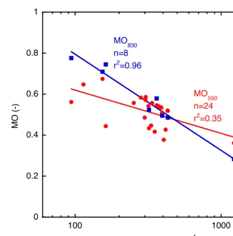
To evaluate Eq. (3), we compare modelled depths of the 550 and 830 kg m−3 density layers (z550 and z830, respec-tively) to observations at 62 firn core locations around the Greenland Ice Sheet (see Sect. 2.4). As we find a system-atic departure of the modelled values, we introduce a cor-rection term MO, defined as the ratio of modelled and ob-served values of z550 and z∗830 (Ligtenberg et al., 2011), wherez∗830=z830−z550. Figure 1 shows MO as a function of
˙
b. As the MO values need to represent dry compaction, we selected 22 firn cores with little surface melt. Linear least-squares fitting then yields the following MO relations for Greenland:
MO550=1.042−0.0916 ln(b)˙ for ρ≤550 kg m−3, (4) MO830=1.734−0.2039 ln(b)˙ for ρ >550 kg m−3. (5) The coefficients in these two equations are different from a previous application in Antarctica (Ligtenberg et al., 2011). We use these updated coefficients to improve the fit with ob-served density profiles. There is no physical interpretation for these coefficients to be different. The different set of coeffi-cients for Greenland and Antarctica could point to a process not presently captured in the model (that happens to corre-late with accumulation rate). Alternatively, the coefficients could be different because the range of accumulation rates on which the Antarctic parameterization (Ligtenberg et al.,
0 0.2 0.4 0.6 0.8 1 100 1000 MO (-)
Mean accumulation (mm y-1) MO830
n=8 r2=0.96
MO550 n=24 r2=0.35
Figure 1. Ratio of modelled vs. observedz550and z∗830(MO550 (red circles and fit line) and MO830 (blue squares and fit line), respectively) for 24 dry firn cores (8 of which are deep enough to include z∗830), as a function of mean annual accumulation (in mm yr−1).
2011) is based is biased to lower accumulation rates than those found in Greenland.
Equation (3) is multiplied with the correction factors MO in Eqs. (4) and (5), which are not allowed to be smaller than 0.25 (Ligtenberg et al., 2011). The accurate performance of these densification expressions is further demonstrated by fully independent comparisons against in situ (Larson et al., 2015) and remotely sensed (Ligtenberg et al., 2015) den-sification rates. However, the use of a mean value of b˙ in these equations has an important limitation: in reality, com-paction is determined by the overburden pressure of the over-lying snow. By using a constant meanb˙ rather than the in-stantaneous overburden pressure, the firn compaction vari-ability is dampened significantly. Following an accumula-tion event, the model only takes into account the increase in compactable material, not the effect of increased overburden pressure on the underlying firn.
Rain is added to the surface snowmelt flux. This liquid wa-ter is allowed to percolate into the firn. Each layer has a max-imum irreducible water contentWc, depending on the density (Coléou and Lesaffre, 1998). Meltwater will refreeze as soon as it encounters a layer that can accommodate both the space of the refreezing water and the latent heat that is released upon refreezing. For details see Ligtenberg et al. (2011) and Kuipers Munneke et al. (2015).
(den-sityρi). UsingWcfrom Coléou and Lesaffre (1998) (which can vary with depthz), it can be shown that the firn air con-tentF (in m) is given as
F = zi Z
0
ρi−ρ(z)
ρi/(1−Wc(z))−ρwWc(z)/(1−Wc(z))−ρa dz.
(6) Here, we will approximate this general expression by assum-ing thatρaρiand thatWc(z)=0, yielding
F = zi Z
0
ρi−ρ(z)
ρi
dz. (7)
As an extreme example, a uniform value ofWc=0.10 (i.e. 10 % of pore space filled with water throughout the firn col-umn) yields a 10 % overestimation ofF.
The firn model is also used to simulate surface eleva-tion changes h˙
f in the ablation area. Here, the prescribed RACMO2.3 mass fluxes determine the ice ablation rate as-suming the ice densityρi. Section 2.3 describes the method to derive the SMB-induced surface elevation changeh˙fin the ablation area.
2.2 Model forcing from RACMO2.3
At the upper boundary of the 1-D firn column, the firn model is forced with surface temperature and mass fluxes from RACMO2.3 (Noël et al., 2015), a regional climate model that is adapted to simulate climatic conditions over ice sheets. The horizontal spatial resolution of RACMO2.3 is 11 km. Forcing data are available for the period 1 January 1960– 31 December 2014, in time steps of 6 h.
RACMO2.3 supersedes RACMO2.1 (Ettema et al., 2010; van Angelen et al., 2012). In the new version, the cloud mi-crophysics, surface and boundary layer turbulence, and radi-ation transport have been updated (van Wessem et al., 2014). The most pronounced effect of these updates on the SMB is an increase in summer snowfall events, decreasing the amount of snow and ice melt in the percolation and ablation area (Noël et al., 2015). The agreement between RACMO2.3 SMB and mass balance stakes in these areas is improved. The ELA is lower and in better agreement with observations. This is expected to improve the description of firn processes in the percolation area of the ice sheet.
2.3 Modelling strategy
While RACMO2.3 itself contains a multi-layer snowpack with the same compaction and meltwater routines as the firn model, the rationale for using an offline firn model is the abil-ity to spin up the firn layer with a reference climate until it is in equilibrium with that reference climate. This circumvents the difficult task of assuming an initial condition of the firn
layer at the start of the RACMO2.3 simulation that is suf-ficiently accurate for correctly determiningh˙
f. Furthermore, because of its computational demands, RACMO2.3 cannot be used for sensitivity tests, in contrast to an offline firn model. Finally, the vertical resolution is higher in the offline model.
Still, the spin-up procedure requires that we define a ref-erence climate, i.e. a period of time in which the properties of neither the firn nor the reference climate forcing exhibit significant trends. Recent modelling and observations reveal that the Greenland Ice Sheet SMB has decreased since the beginning of the 1990s (e.g. Shepherd et al., 2012; Ender-lyn et al., 2014). As a result, thinning has increased sharply since the mid-1990s (Csatho et al., 2014) along the margins of the ice sheet. Clearly, the reference period should not in-clude this period and should end preferably some years be-fore its onset. Therebe-fore, our modelling strategy is that we choose the first 20 years of RACMO2.3 forcing data (1 Jan-uary 1960–31 December 1979) and spin up the firn column at each location with a loop over this 20-year period until the properties of the firn layer have converged to an equi-librium. By doing so, we assume that the pre-1960 climate (i.e. the reference climate) can be represented by a sequence of 20-year periods. In practice, equilibrium is reached when all the mass in the firn layer is refreshed once following the start of the spin-up. The duration of the spin-up is therefore computed as the thickness of the firn layer (from the surface to the depth at which the ice density is reached) divided by the mean annual accumulation rate. A major uncertainty in the calculated firn depth changes in this study stems from this assumption of reference climate. We will quantify this uncertainty in Sect. 4.4.
As a second important assumption, we set the surface el-evation change h˙f over the reference period to zero. After all, the modelled firn layer at the end of the reference period (31 December 1979) is the result of the spin-up procedure that uses multiple loops over the reference period to reach an equilibrium state, plus 20 years of model integration using the same data as in the spin-up procedure. For the accumula-tion area, it means that the amount of mass leaving the bot-tom of the firn layer (with a velocityvice) is assumed equal to the total mass added to and retained in the firn column by snowfall and refreezing, minus run-off.
For the ablation area, the assumption ofh˙f=0 during the reference period implies that the downward velocity from a negative SMB (ablation) is balanced by an upward and equal flux of emergent ice. The emergent ice flux is repre-sented by the termvice. In Eq. (1), we setvice equal to the opposite sign of the sum of all other velocity components for the reference period. Thereafter,vice retains the same value, but the other parameters are free to evolve. In this framework,
˙
reference period: it can change due to ice-dynamical thin-ning or thickethin-ning. Only the ablation-driven surface eleva-tion changeh˙fis assumed to be zero.
Note that our choice of the period 1960–1979 for a rep-resentative reference climate implies that modelled surface elevation after 1980 is allowed to evolve freely due to SMB and firn processes. It is not bounded by the requirement that
˙
hfshould be zero over the entire simulation period, like in studies addressing the Antarctic Ice Sheet (Ligtenberg et al., 2011; Pritchard et al., 2012). As the firn layer starts to evolve freely from 1980 onwards, we present time series starting in 1980, although the complete time series of elevation change start in 1960.
2.4 Firn cores
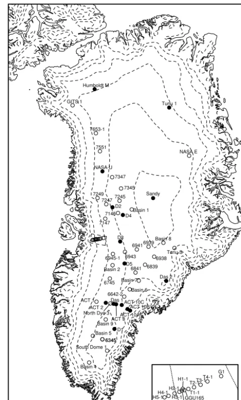
To evaluate the firn model, we collected vertical profiles of firn density from 62 shallow cores from widely varying loca-tions across the Greenland Ice Sheet (see the map in Fig. 2), drilled between 1995 and 2012. Among the cores are those drilled for PARCA (Program for Arctic Regional Climate Assessment; McConnell et al., 2000b; Mosley-Thompson et al., 2001; Hanna et al., 2006; Banta and McConnell, 2007); cores from the Arctic Circle Traverses (ACT; Box et al., 2013); cores from the lower part of the EGIG line (Harper et al., 2012); and Das 1 and Das 2 (e.g. Hanna et al., 2006).
Vertical profiles of density from firn cores are usually based on the mean density of 0.5–2 m long sections. Some researchers log the midpoint of each section as the depth of the section; others use the top or the bottom of the section. Here, all 62 profiles have been interpolated to give the mean density at the midpoints of each core section. For each core, the collection date is known, and vertical profiles of modelled firn density are extracted from the model at the time closest to the collection date, and from the nearest model grid cell.
2.5 Laser altimetry
Since 1992, NASA’s Airborne Topographic Mapper (ATM) has carried out laser surveys of the Greenland Ice Sheet sur-face. If sufficient repeat observations are available, a time se-ries of observed surface elevation change can be constructed, spanning the period 1992–2013.
To do so, we use the Level 2 “Qfit” product, which pro-vides the waveform-fitted elevations for the centroid of each laser return. In order to derive elevation changes, we inter-polated the Qfit point cloud for each campaign to a refer-ence grid with 30 m spacing. We then selected referrefer-ence grid points with at least one observation in each of five epochs: 1993–1996, 1997–2000, 2001–2005, 2006–2009, and 2010– 2013. Of these points, we selected 15 within the central and northern interior of the ice sheet, where a relatively small contribution of ice dynamics is expected. Based on differ-ences in elevation obtained from crossovers within a few weeks, we estimate 1σ errors in the elevation observations
Figure 2. Map of Greenland showing the 62 firn cores used for validation of the firn model. Solid circles represent firn cores longer than 30 m; open circles are firn cores shorter than 30 m. The inset in the lower right shows cores from Harper et al. (2012) in the west Greenland percolation area around 69◦420N. Dashed contours are surface elevation isolines with a spacing of 500 m, the uppermost being 3000 m.
to be±10 cm, which includes interpolation error. Results of the comparison between the firn model and the ATM data are found in Table 1 and Fig. 5.
3 Model evaluation
3.1 Vertical profiles of density
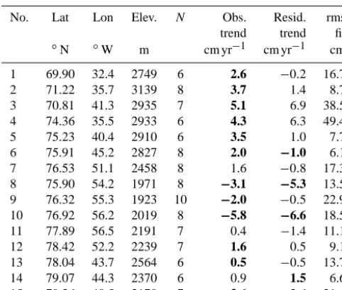
Table 1. Coordinates of analysed elevation change points labelled in Fig. 5 with the number of repeat observationsN, observed sur-face elevation trend from the laser altimetry, the best-fit trend in the residuals between the observations and the firn model heights, and the root mean square of the residuals between the observations and fitted model (in cm). Trends in bold are significantly different than zero at 95 % confidence.
No. Lat Lon Elev. N Obs. Resid. rms trend trend fit ◦
N ◦W m cm yr−1 cm yr−1 cm
1 69.90 32.4 2749 6 2.6 −0.2 16.7
2 71.22 35.7 3139 8 3.7 1.4 8.7
3 70.81 41.3 2935 7 5.1 6.9 38.5
4 74.36 35.5 2933 6 4.3 6.3 49.4
5 75.23 40.4 2910 6 3.5 1.0 7.7
6 75.91 45.2 2827 8 2.0 −1.0 6.1
7 76.53 51.1 2458 8 1.6 −0.8 17.3 8 75.90 54.2 1971 8 −3.1 −5.3 13.5 9 76.32 55.3 1923 10 −2.0 −0.5 22.9 10 76.92 56.2 2019 8 −5.8 −6.6 18.5 11 77.89 56.5 2191 7 0.4 −1.4 11.1
12 78.42 52.2 2239 7 1.6 0.5 9.1
13 78.04 43.7 2564 6 0.5 −0.5 13.7
14 79.07 44.3 2370 6 0.9 1.5 6.6
15 79.36 48.5 2170 7 3.6 2.6 21.6
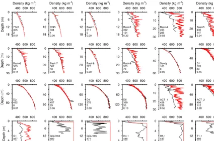
density levels from these cores to tune the densification pa-rameterization in Eqs. (4) and (5). Still, we can compare the shape of the profiles beyond these two levels, and we can as-sess the impact of melt and refreezing on the vertical density profile.
Figure 3 shows the observed and modelled density profiles for all core locations. Each panel includes the mean accu-mulation and melt from RACMO2.3 (in mm yr−1) for 1960– 2014, and the ratioRmaof these melt and accumulation av-erages.
The vertical resolution of the firn core data is typically 0.5–2.0 m, thereby smoothing out the effect of ice lenses and higher-density layers. The model data in Fig. 3 are shown at full resolution, i.e. with layers of 5–10 cm thickness. The high-density layers usually represent thick layers of refrozen meltwater with a density close to that of solid ice.
Up to anRmavalue of 0.3–0.4, the agreement between the firn model and the observations is good. But for higherRma, the firn model starts to overestimate the density throughout the firn column. Figure 4 compares the observed and mod-elled firn air contentF, showingRmain colour. The model bias clearly increases for higherRma. This means that there are three possible causes for the misfit, which are not mutu-ally exclusive: (1) RACMO2.3 simulates too much melt in the percolation areas, causing the firn to fill up quickly with too much refrozen meltwater; (2) RACMO2.3 simulates too little accumulation, providing insufficient pore space to store meltwater; and (3) the firn model should allow for more and
more rapid downward percolation of meltwater without let-ting it refreeze.
Regarding a possible overestimation of melt in RACMO2.3, there is limited evidence that the amount of melt observed by an automatic weather station at location S10 (67◦000N 47◦010W, 1850 m a.s.l.) is indeed about 20 % smaller than simulated by RACMO2.3 (Noël et al., 2015). Further north, Harper et al. (2012) find the equilibrium line around the EGIG line at about 1100–1200 m a.s.l., while the equilibrium line altitude in RACMO2.3 is at∼1650 m a.s.l., about 45 km further inland. For firn cores H1-1 down to H5-1 (Fig. 2), it is clear that under RACMO2.3 forcing (with melt larger than accumulation) a firn layer cannot be sustained, whereas in reality there is a shallow firnpack with infiltration ice layers. There is very limited reliable infor-mation about melt fluxes from other parts of the percolation area around the ice sheet, so we cannot conclude whether the overestimation of modelled melt flux is structural.
The other possible source for the misfit is the percola-tion scheme in the firn model itself. The firn model adopts a so-called “tipping bucket” approach, where meltwater is allowed to move downward from one discrete layer to the next whenever the first layer is saturated. In practice, the per-colation is more complex, and vertical meltwater transport through confined channels (pipes) is known to occur (Marsh and Woo, 1984; Humphrey et al., 2012). Piping of meltwater is a way to evacuate more meltwater towards the bottom of the firn layer, reducing the amount of refreezing in the firn itself. Alternatively, intermediate-thick ice layers may serve as an impermeable surface along which the water can run off. Both processes increase the run-off and decrease refreezing and density. At present, we cannot assess the performance of the firn model in more detail, since we cannot easily isolate it from errors in the model forcing from RACMO2.3.
It is unclear what exactly the model bias in the percola-tion zone implies for the modelled rates of surface elevapercola-tion change. We speculate that, if too much refreezing is the cause for the density overestimation, then a prescribed increase in surface melt would underestimate the rate of surface lower-ing.
3.2 Altimetry from the high-elevation interior
In the high interior of the Greenland Ice Sheet, horizontal surface ice velocities are low (generally less than 10 m yr−1; Joughin et al., 2010), and elevation changes resulting from ice-dynamical effects are expected to be small. Figure 5 shows time series of observed surface elevation change from the ATM lidar, along with the surface elevation change pre-dicted by the firn model.
Figure 3. Observed (black) and modelled (red) firn density profiles for 24 of the 62 firn cores on the Greenland Ice Sheet. The four lines of text in each panel show (1) the core name, (2) mean annual accumulation and (3) melt (in mm w.e. yr−1) from RACMO2.3, and (4) the ratio of these fluxes (Rma, dimensionless). Remaining profiles are shown in Appendix A as Figs. A1 and A2.
Figure 4. Modelled vs. observed firn air contentF (in m) for 59 of the 62 firn cores (cores H2-1, H3-1, and H4-1 are not shown). The colour scale to the right indicates the ratio of modelled mean melt and accumulation fluxesRma, and the colour of each dot in the scatter plot corresponds to the value ofRmafor that firn core location.
0.05
-0.05 0
(m y-1)
Δ
El
e
va
ti
o
n
(m)
Year 1
2 3
4 5 6 7 8 9 10
1112 13
1514
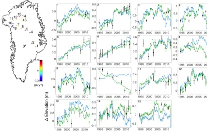
Figure 5. Upper left panel: map of elevation change points observed by the airborne laser altimeter ATM, with colour scale giving the 20-year trend in elevation (m yr−1). The 15 panels (numbers in the upper left corner of each panel correspond to the numbered locations on the map) show surface elevation change from (black dots with 1σ error bars) ATM lidar and (blue curves) firn thickness model. Green curves are the firn model results adjusted to the trend in residuals between the model and the observations.
residuals of 1 cm yr−1opposes the 2 cm yr−1of observed sur-face raising, suggesting opposing contributions from dynam-ics and accumulation. At sites 8 and 10, the strongly negative trend in residuals is larger than the observed surface lower-ing, indicating that increased accumulation is partially off-setting relatively rapid dynamic thinning.
If the trend in residuals between the observed and mod-elled surface elevations provides the linear contribution in ice dynamics plus the error, the error is then assessed by the root mean square (rms) of the detrended residuals (Table 1). This is equivalent to adjusting the firn model time series to the ice-dynamical trend (shown as green curves in the pan-els of Fig. 5) and computing the difference from the obser-vations. The mean rms error is 17.4 cm, which is close to the lidar observational uncertainty (∼10 cm). Sites 3 and 4 have the largest errors, reaching 1.7 and 2.6 standard devi-ations, respectively. These sites are located at similar eleva-tions (2930 m) on the central eastern portion of the ice sheet, where altimetry shows steadily increasing elevations while the firn model predicts an initial increase in firn thickness until about 2005 and then a decrease thereafter.
4 Elevation change due to firn and SMB 4.1 Firn air content
Figure 6 shows the modelled firn air contentF on 1 Septem-ber 2014. As noted in Sect. 3, these values are probably real-istic in the dry interior and the upper part of the percolation area. In the lower percolation area, where the annual melt flux exceeds ∼30 % of the annual accumulation rate, the modelled firn air content is likely underestimated. Around the central dome, we find the highest values ofF of about 25 m. There is a remarkable contrast between the firn in the NW and the NE, with the NW having higherF. This can be explained by more snowfall in the NW and higher sublima-tion in the NE due to a lower relative humidity.
4.2 Trends
Figure 6. Modelled firn air contentFon 1 September 2014 (in m). Dashed contour lines at 500 m height intervals.
firn and SMB processes) is assumed. Again, there is a pro-nounced pattern of modest thickening of the firn layer in the interior (most notably towards the east) and moderate to strong thinning of the firn layer around the margins. The inte-rior thickening is of the order of 1–5 cm yr−1, or 34–170 cm, over the entire 34-year period. The marginal thinning rates are much larger; they can be up to 20–50 cm yr−1, or 6–18 m, over the entire period, with the highest values in the south-east. In contrast to the Summit dome firn layer, that of the southern dome of the Greenland Ice Sheet is thinning.
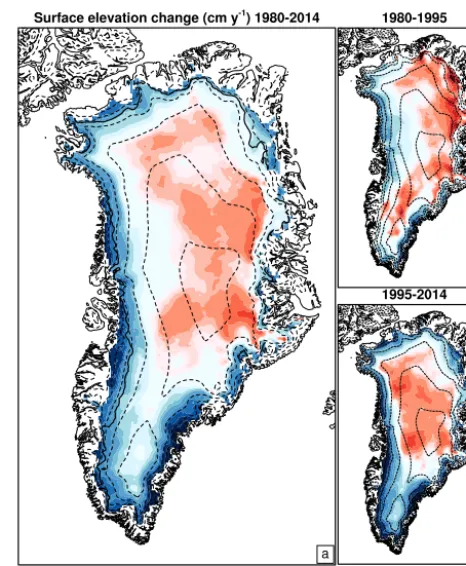
It is clear that the patterns have changed over this period. The surface elevation change map over 1980–1995 (Fig. 7b) shows thinning along the southeast, south, west, and north-west coasts. Thickening is occurring in the interior (mainly east of the divide) and along the north and northeast coasts. Since 1995, thinning has intensified and spread over the en-tire coastal margin. The thickening moved to the west of the interior. The aggregate picture for the period 1980–2014 then shows moderate thickening up to 5 cm yr−1 in the eastern and northern interior. Thinning occurs all around the mar-gins, with the smallest rates (0–15 cm yr−1) in the north-ern and eastnorth-ern coastal regions. The largest rates (exceeding 40 cm yr−1) occur in the southeast and in the western ablation area.
Figure 7. Modelled average firn thickness changeh˙(in cm yr−1) for three periods: (a) 1980–2014, (b) 1980–1995 and (c) 1995–2014. The equilibrium line (according to the RACMO2.3 SMB) is shown as a thick black line in (a). Note that the colour scale is asymmetric around 0. In the ablation area, where no firn layer is present, ice thickness change by surface processes is presented.
4.3 Decomposing the trends
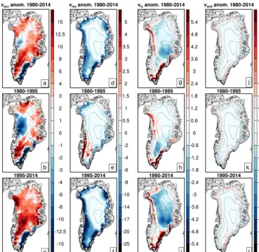
The firn model allows for a decomposition of theh˙fsignal into its velocity components (Eq. 1). The upper panels in Fig. 8 show this decomposition for the period 1980–2014. The thickening in the eastern interior (Fig. 7a) can be almost fully ascribed to a positive accumulation anomaly (Fig. 8a), offset by a small increase in firn compaction due to this extra firn (Fig. 8g). In the lower accumulation area, the positive ac-cumulation anomaly is offset by a significant increase in sur-face melt, giving zero or slightly negativeh˙fin the western percolation area. In the south, increased surface melt dom-inates the thinning signal, whereas accumulation, firn com-paction, and snowdrift anomalies play a minor role. In the southeast, melt has increased and accumulation decreased significantly. As the absolute values of both accumulation and melt are large in this region, we find here the largest rates of firn-driven surface lowering seen in Greenland.
Figure 8. Anomaly of vertical velocity components with respect to the reference period 1960–1979 (in cm yr−1). (a–c) Accumulation velocity
vacc; (d–f) melt velocityvme; (g–i) firn compaction velocityvfc; (j–l) snowdrift sublimation, erosion and deposition velocities (vsnd+ver). Note that the colour scales forvmeis strongly asymmetric around 0.
of significant melt anomalies (panel e), the thickening in the eastern and northeastern interior can be almost fully ascribed to a positive accumulation anomaly (panel b). This is mir-rored in a small negative firn compaction anomaly (panel h). Over almost the entire ice sheet, with the exception of the southeast, the period 1995–2013 shows a positive accumula-tion anomaly (panel c). At lower elevaaccumula-tions however, the firn thickness change is dominated by the strong melt anomaly over this period (panel f).
The velocity components that always lead to a decrease of ˙
hf, melt and firn compaction, are negative by definition. To complement this, we can add up the snowdrift and surface sublimation velocities whenever they lead to a surface lower-ing. The partitioning of the surface lowering into these com-ponents of negative velocities is shown in Fig. 9. The lower-ing is dominated by firn compaction (panel b) in the interior and more and more by melt around the margins. There, the firn layer is thinner, which reduces the compaction potential. In the dry northeast, there is a relatively large contribution
from sublimation (up to 30 %, panel d). This is caused by a combination of strong winds and a relatively low humidity, promoting snowdrift sublimation. For another part, the rel-ative contribution increases as the firn compaction is small due to lower firn temperatures, and due to the relatively small thickness of the firn layer.
4.4 Error estimate
Figure 9. Fraction of surface lowering (negative velocities only) during 1980–2014 caused by (a) melt; (b) firn compaction; (c) snowdrift processes; and (d) sublimation. Up to a fraction of 0.15, the colour scale is divided in steps of 0.025. Above 0.15, the step size is 0.05.
larger than the long-term average. Other reconstructions show the 1960–1979 solid precipitation flux to be 0–10 % different from the period between∼1850 and the present day (Wake et al., 2009; Hanna et al., 2011). For the error analy-sis, we therefore assume that the 1960–1979 accumulation fluxes (precipitation minus evaporation/sublimation) can dif-fer by up to 15 % from the long-term accumulation history. We denote this accumulation uncertainty byσb˙(in mm yr−1).
For snowmelt, we also assume a maximum deviation of 15 % of the 1960–1979 melt flux compared to the long-term history. There is limited evidence for this, but according to reconstructions from Hanna et al. (2011) the run-off flux for 1960–1979 differs about 5–10 % from the 1870–2010 mean. This uncertainty is given asσm˙ (mm yr−1).
For the suite of 62 firn core locations, we perform four sensitivity tests, in which we increase and decrease melt or accumulation by 15 % after completion of the spin-up. The resulting drift inh˙ffor 1960–2014 gives an error in the firn thickness change. The error in surface elevation change due toσb˙is written asσh,˙b˙. Analogously, the error in surface
el-evation change due toσm˙ is given asσh,˙m˙. By relatingσh,˙b˙
and σh,˙m˙ empirically to accumulation and melt at the core
locations, we can expand the error product over the entire ice sheet. These relations are
σh,˙b˙=σb˙(0.107+3.609×10⁴b),˙ (8)
σh,˙m˙=σm˙(0.225+1.064×10³m),˙ (9)
withb˙andm˙ in millimetres per year.
The uncertainties σb˙ andσm˙ cannot be regarded as
inde-pendent. The SMB module in RACMO2.3 contains interac-tions between accumulation and melt. We identify the melt-albedo feedback as the most important interaction. As an example, a negative bias in summer snowfall could lead to an excess of summer melt because albedo will be underesti-mated. To capture this dependence in the error analysis, we assume the errors in surface elevation change due to
uncer-Figure 10. Estimate of errors in firn thickness change (cm yr−1). (a) Errorσh,˙b˙ due to accumulation uncertaintyσb˙; (b) errorσh,˙m˙ due to melt uncertaintyσm˙; and (c) total errorσh˙. Note the non-linear colour scale.
tainties in the melt and accumulation fluxes to be dependent, and we add them up linearly (σh˙=σh,˙b˙+σh,˙m˙).
The resulting total error and its components are shown in Fig. 10. In the interior, the total error (panel c) is under-standably dominated by the accumulation uncertainty (panel a). Towards the ice-sheet edge, the melt uncertainty (panel b) starts to dominate the total uncertainty. The total uncer-tainty increases from 0.2–1.0 cm yr−1 in the interior to 10– 20 cm yr−1 in the lower percolation area. The largest total error (more than 40 cm yr−1) is found in the southeast, where high snowfall rates coincide with large amounts of melt.
to more snowfall is partially offset by a more rapid densi-fication. For b >˙ 2427 mm yr−1, the term between brackets in Eq. (8) becomes larger than unity. There is no physical explanation for this behaviour: it is caused by the empiri-cal nature of Eq. (8). However, we decided not to cap the uncertainty, for the following reason: the densification rate in Eq. (3) depends on a 20-year mean accumulation rate, whereas true densification at a particular depth in the firn de-pends on the immediate overburden pressure from overlying firn, which can be more variable than the long-term mean. This was already shown to dampen the modelled variability in densification rate compared to observations (Ligtenberg et al., 2015). Therefore, the observed, short-term firn thick-ness change variability could be of the same order of magni-tude as the accumulation rate variability for large accumula-tion rates.
4.5 Integrated volume change
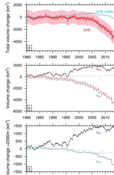
Figure 11 shows the cumulative volume change of the Green-land Ice Sheet as a consequence of changes in firn and SMB processes. Until the late 1990s, the total volume change was small. Since 2000, the total volume has decreased by about 3295±1030 km3due to firn and SMB processes alone. Av-eraged over the ice sheet, this is a mean surface lowering of 1.96±0.61 m. Almost all of this total volume loss took place in the part of the Greenland Ice Sheet where the surface is under 2000 m a.s.l.
Panels b and c of Fig. 11 show the partitioning of the vol-ume change for the entire ice sheet and the part elevated above 2000 m a.s.l., respectively. Over 1980–2014, the vol-ume loss through melt was slightly over 4700 km3. This loss was partly compensated for by an increase in snow accumu-lation of about 1500 km3. On most of the ice sheet, firn com-paction has accelerated (become more negative) due to an increase in accumulation. Above 2000 m, the effect is clearly visible (Fig. 11c). Integrated over the ice sheet however, we see a small slowdown in firn compaction, corresponding to about 500 km3 (Fig. 11b). The firn compaction anomaly is dominated by the southeastern part of the ice sheet, where snowfall has decreased strongly in an absolute sense (less so in a relative sense) and firn compaction has slowed down (Fig. 8h and i).
Up to about 2005, firn volume change above 2000 m a.s.l.
was dominated by accumulation variability (consistent with e.g. McConnell et al., 2000a), and below 2000 m a.s.l. the volume change was mainly melt-driven. This is consistent with the original speculation in early reports of what would happen to the Greenland Ice Sheet in response to global warming. After 2005 however, the total firn volume above 2000 m a.s.l.has started to decrease, mainly because surface melt has migrated inland (e.g. Fettweis et al., 2011), but also because the accumulation increase, clearly visible be-tween 1980 and 2000, stagnated in the 2000s. It remains to be seen if the paradigm of interior thickening under
atmo-Figure 11. (a) Ice-sheet-integrated volume change for 1980–2014 (in km3) due to firn and SMB processes. The thin red line is the vol-ume change based on weekly output from the firn model; the thick red line is a 1-year running average; and the pink shaded area shows the uncertainty estimate. The blue line shows the volume change for the part of the ice-sheet surface elevated more than 2000 m a.s.l.
(b) Partitioning of the total volume change into the three main components: accumulationvacc, meltvme, and firn compactionvfc. (c) Like (b) but for the ice sheet higher than 2000 m a.s.l.
spheric warming can stand up against the inland migration of the area of surface melt.
4.6 Altimetry correction and mean density of firn-related mass loss
The present data set of firn thickness and mass change is primarily aimed at the correction of altimetry prod-ucts, allowing for the extraction of an ice-dynamical thin-ning/thickening signal. The procedure for doing so is as fol-lows: suppose that an altimetry sensor measures a surface el-evation change h(t˙ 0, t1)≡(h(t1)−h(t0))/(t1−t0)between initial time t0 and time t1> t0. The firn model computes a surface elevation change due to firn and SMB processes
˙
hf(t0, t1)≡hf(t1)−hf(t0). The supposed ice-dynamical con-tribution (neglecting vertical bed movement, but this could be included; Sørensen et al., 2011) is thenh˙d= ˙h− ˙hf. The associated mass changem˙dis simply computed as
˙
md=ρih˙d. (10) The mass changem˙dis caused by horizontal convergence or divergence of ice flux, arising from, e.g., ice-flow accelera-tion propagating from the margin, long-term changes in the ice-sheet viscosity (Colgan et al., 2015), and transient varia-tions in ice flow due to long-term changes in accumulation. The mass change due to the SMB,m˙f, is computed directly from the RACMO2.3 forcing, using SMB anomalies with re-spect to the appropriate reference period (1960–1979). This is by far the simplest approach and completely consistent with the firn model that uses the same forcing and the same reference period. The total mass change at the given location
˙
mis then computed as ˙
m= ˙md+ ˙mf. (11)
5 Conclusions
In this study, we used a time-dependent, semi-empirical model for firn compaction, meltwater percolation, and re-freezing. We forced the model with surface mass fluxes and temperature from the regional climate model RACMO2.3 for the period 1960–2014. By forcing the model with all mass fluxes, including melt, the result is a data series of surface elevation change over the entire ice sheet, due not only to firn processes but also to anomalies in the SMB. We defined a reference period from 1960 up to and including 1979, in which we assumed the surface elevation change to be zero due to firn and SMB processes. In the ablation zone, the computed surface elevation change represents the ablation anomaly with respect to the 1960–1979 mean ablation.
The firn model was calibrated against vertical profiles of firn density from more than 60 shallow and deep firn cores collected around Greenland in the past 2 decades. This en-sured a very good agreement between observed and mod-elled vertical density profiles, especially in regions where the annual surface melt flux is small (less than about 20 %) compared to the mean annual accumulation. In regions with higher melt, the firn model overestimates the density be-low the surface. Potentially, this underestimates the presented rates of surface lowering in the percolation area.
The computed surface elevation change was compared against lidar observations of surface elevation change at loca-tions where we expect the ice-dynamical changes to be small or gradual in time. At most locations, we find a good fit of the modelled elevation change rates to the observed ones.
Between 1980 and 2014, we see a pronounced pattern of small thickening of the firn layer in the high interior, of 1 to 5 cm yr−1, caused predominantly by an accumulation in-crease over this period. Around the margins of the ice sheet, in the percolation and ablation areas, the surface is lowering, at rates of up to 20–50 cm yr−1. This is mostly caused by an increase in surface melt, augmented in the southeast by a de-crease in accumulation of snow. The thinning signal in the margins of the ice sheet has accelerated between 1980 and 2014, in line with observations of increased surface melt.
During the period 1980–2014, the surface elevation in-crease in the interior shifted from the east and northeast to-wards the centre of the ice sheet and stagnated toto-wards the end of the time series. The contribution from surface melt to interior surface lowering has increased markedly in this period, with the largest firn volume decrease due to surface melting in the extreme melt summer of 2012.
Appendix A: Remaining vertical profiles of firn density Here, we present the remaining 33 vertical profiles of firn density, in addition to the 24 firn cores shown in Fig. 3. They are shown in Figs. A1 and A2.
Figure A1. Observed (black) and modelled (red) firn density profiles for 24 of the 62 firn cores on the Greenland Ice Sheet. The four lines of text in each panel show (1) the core name, (2) mean annual accumulation and (3) melt (in mm w.e. yr−1) from RACMO2.3, and (4) the ratio of these fluxes (Rma, dimensionless). The other vertical profiles are shown in Figs. 3 and A2.
Author contributions. P. Kuipers Munneke carried out the model experiments and analysis, and wrote the paper; S. R. M. Ligtenberg co-developed the firn model; B. P. Y. Noël provided the RACMO2.3 forcing data; I. M. Howat provided ATM altimetry data and con-tributed to the writing; J. E. Box concon-tributed firn core data and his-torical accumulation data; E. Mosley-Thompson, J. R. McConnell, K. Steffen, J. T. Harper and S. B. Das provided firn core data; and M. R. van den Broeke conceived this study. All authors reviewed and commented on the manuscript.
Acknowledgements. P. Kuipers Munneke received financial
support from the Netherlands Polar Programme (NPP) of the Netherlands Institute for Scientific Research (NWO). ECMWF at Reading (UK) is acknowledged for use of the Cray supercomputing system. Graphics were made using the NCAR Command Language (version 6.2.1, 2014). The J. E. Box contribution is supported by Det Frie Forskningsråd grant 4002-00234 and Geocenter Denmark.
Edited by: J. L. Bamber
References
Arthern, R. J., Vaughan, D. G., Rankin, A. M., Mulvaney, R., and Thomas, E. R.: In situ measurements of Antarctic snow com-paction compared with predictions of models, J. Geophys. Res., 115, F03011, doi:10.1029/2009JF001306, 2010.
Banta, J. R. and McConnell, J. R.: Annual accumulation over recent centuries at four sites in central Greenland, J. Geophys. Res.-Atmos., 112, D10114, doi:10.1029/2006JD007887, 2007. Benson, C. S.: Stratigraphic studies in the snow and firn of the
Greenland ice sheet, SIPRE Research Report 70, US Army Cold Regions Research and Engineering Laboratory (CRREL), Hanover, USA, 1962.
Box, J. E., Cressie, N., Bromwich, D. H., Jung, J.-H., Van den Broeke, M. R., Van Angelen, J. H., Forster, R. R., Miège, C., Mosley-Thompson, E., Vinther, B., and McConnell, J. R.: Greenland Ice Sheet mass balance reconstruction, Part I: net snow accumulation (1600–2009), J. Climate, 26, 3919–3934, doi:10.1175/JCLI-D-12-00373.1, 2013.
Braithwaite, R. J., Laternser, M., and Pfeffer, W. T.: Variations of near-surface firn density in the lower accumulation area of the Greenland ice sheet, Pâkitsoq, West Greenland, J. Glaciol., 40, 477–485, 1994.
Brown, J., Bradford, J., Harper, J., Pfeffer, W. T., Humphrey, N., and Mosley-Thompson, E.: Georadar-derived estimates of firn density in the percolation zone, western Greenland ice sheet, J. Geophys. Res.-Earth, 117, F01011, doi:10.1029/2011JF002089, 2012.
Coléou, C. and Lesaffre, B.: Irreducible water saturation in snow: experimental results in a cold laboratory, Ann. Glaciol., 26, 64– 68, 1998.
Colgan, W., Box, J. E., Andersen, M. L., Fettweis, X., Csathó, B., Fausto, R. S., Van As, D., and Wahr, J.: Greenland high-elevation mass balance: inference and implication of refer-ence period (1961–90) imbalance, Ann. Glaciol., 56, 105–117, doi:10.3189/2015AoG70A967, 2015.
Csatho, B. M., Schenk, A. F., van der Veen, C. J., Babonis, G., Duncan, K., Rezvanbehbahani, S., Van den Broeke, M. R., Simonsen, S. B., Nagarajan, S., and Van Angelen, J. H.: Laser altimetry reveals complex pattern of Greenland Ice Sheet dynamics, P. Natl. Acad. Sci. USA, 111, 18478–18483, doi:10.1073/pnas.1411680112, 2014.
Davis, C. H., Li, Y., McConnell, J. R., Frey, M. M., and Hanna, E.: Snowfall-driven growth in East Antarctic ice sheet mitigates re-cent sea-level rise, Science, 308, 1898–1901, 2005.
Enderlyn, E. M., Howat, I. M., Jeong, S., Noh, M.-J., Van Ange-len, J. H., and Van den Broeke, M. R.: An improved mass budget for the Greenland ice sheet, Geophys. Res. Lett., 41, 866–872, doi:10.1002/2013GL059010, 2014.
Ettema, J., Van den Broeke, M. R., Van Meijgaard, E., Van de Berg, W. J., Box, J. E., and Steffen, K.: Climate of the Greenland ice sheet using a high-resolution climate model – Part 1: Evalu-ation, The Cryosphere, 4, 511–527, doi:10.5194/tc-4-511-2010, 2010.
Fettweis, X., Tedesco, M., Van den Broeke, M., and Ettema, J.: Melting trends over the Greenland ice sheet (1958–2009) from spaceborne microwave data and regional climate models, The Cryosphere, 5, 359–375, doi:10.5194/tc-5-359-2011, 2011. Gardelle, J., Berthier, E., and Arnaud, Y.: Slight mass gain
of Karakoram glaciers in the early twenty-first century, Nat. Geosci., 5, 322–325, doi:10.1038/ngeo1450, 2012.
Gardner, A. S., Moholdt, G., Cogley, J. C., Wouters, B., Arendt, A. A., Wahr, J., Berthier, E., Hock, R., Pfeffer, W. T., Kaser, G., Ligtenberg, S. R. M., Bolch, T., Sharp, M. J., Ha-gen, J. O., Van den Broeke, M. R., and Paul, F.: A reconciled estimate of glacier contributions to sea level rise: 2003 to 2009, Science, 340, 852–857, doi:10.1126/science.1234532, 2013. Hanna, E., McConnell, J., Das, S., Cappelen, J., and Stephens, A.:
Observed and modelled Greenland Ice Sheet snow accumulation, 1958–2003, and links with regional climate forcing, J. Climate, 19, 344–358, 2006.
Hanna, E., Huybrechts, P., Cappelen, J., Steffen, K., Bales, R. C., Burgess, E., McConnell, J. R., Steffensen, J. P., Van den Broeke, M. R., Wake, L., Bigg, G., Griffiths, M., and Savas, D.: Greenland Ice Sheet surface mass balance 1870 tot 2010 based on twentieth century reanalysis, and links with global climate forcing, J. Geophys. Res.-Atmos., 116, D24121, doi:10.1029/2011JD016387, 2011.
Harper, J., Humphrey, N., Pfeffer, W. T., Brown, J., and Fet-tweis, X.: Greenland ice-sheet contribution to sea-level rise buffered by meltwater storage in firn, Nature, 491, 240–243, doi:10.1038/nature11566, 2012.
Humphrey, N. F., Harper, J. T., and Pfeffer, W. T.: Thermal track-ing of meltwater retention in Greenland’s accumulation area, J. Geophys. Res.-Earth, 117, F01010, doi:10.1029/2011JF002083, 2012.
Hurkmans, R. T. W. L., Bamber, J. L., Davis, C. H., Joughin, I. R., Khvorostovsky, K. S., Smith, B. S., and Schoen, N.: Time-evolving mass loss of the Greenland Ice Sheet from satellite al-timetry, The Cryosphere, 8, 1725–1740, doi:10.5194/tc-8-1725-2014, 2014.
Khan, S. A., Kjær, H. K., Bevis, M., Bamber, J. L., Wahr, J., Kjeldsen, K. K., Bjørk, A. A., Korsgaard, N. J., Stearns, L. A., Van den Broeke, M. R., Liu, L., Larsen, N. K., and Muresan, I. S.: Sustained mass loss of the northeast Greenland ice sheet trig-gered by regional warming, Nat. Clim. Change, 4, 292–299, doi:10.1038/NCLIMATE2161, 2014.
Kjeldsen, K. K., Khan, S. A., Wahr, J., Korsgaard, N. J., Kjær, H. K., Bjørk, A. A., Hurkmans, R., Van den Broeke, M. R., Bam-ber, J. L., and Van Angelen, J. H.: Improved ice loss estimate of the northwestern Greenland ice sheet, J. Geophys. Res.-Earth, 118, 698–708, 2014.
Kuipers Munneke, P., Ligtenberg, S. R. M., Suder, E. A., and Van den Broeke, M. R.: A model study of the response of dry and wet firn to climate change, Ann. Glaciol., 56, 1–14, doi:10.3189/2015AoG70A994, 2015.
Larson, K., Wahr, J., and Kuipers Munneke, P.: Constraints on snow accumulation and firn density in Greenland using GPS receivers, J. Glaciol., 61, 1–14, doi:10.3189/2015JoG14J130, 2015.
Lenaerts, J. T. M., van den Broeke, M. R., Déry, S. J., König-Langlo, G., Ettema, J., and Munneke, P. K.: Modelling snowdrift sublimation on an Antarctic ice shelf, The Cryosphere, 4, 179– 190, doi:10.5194/tc-4-179-2010, 2010.
Li, J. and Zwally, H. J.: Modeling of firn compaction for estimating ice-sheet mass change from observed ice-sheet elevation change, Ann. Glaciol., 52, 1–7, 2011.
Ligtenberg, S. R. M., Helsen, M. M., and van den Broeke, M. R.: An improved semi-empirical model for the densification of Antarc-tic firn, The Cryosphere, 5, 809–819, doi:10.5194/tc-5-809-2011, 2011.
Ligtenberg, S. R. M., Medley, B., Van den Broeke, M. R., and Kuipers Munneke, P.: Antarctic firn compaction rates from repeat-track airborne radar data, part 2: firn model evalua-tion, Ann. Glaciol., 56, 167–174, doi:10.3189/2015AoG70A204, 2015.
Marsh, P. and Woo, M.-K.: Wetting front advance and freezing of meltwater within a snow cover 1. Observation in the Canadian Arctic, Water Resour. Res., 20, 1853–1864, 1984.
McConnell, J. R., Arthern, R. J., Mosley-Thompson, E., Davis, C. H., Bales, R. C., Thomas, R., Burkhart, J. F., and Kyne, J. D.: Changes in Greenland ice sheet elevation attributed primarily to snow accumulation variability, Nature, 406, 877– 879, 2000a.
McConnell, J. R., Mosley-Thompson, E., Bromwich, D. H., Bales, R. C., and Kyne, J.: Interannual variations of snow accu-mulation on the Greenland Ice Sheet (1985–1996), J. Geophys. Res., 105, 4039–4046, 2000b.
Moholdt, G., Wouters, B., and Gardner, A. S.: Recent mass changes of glaciers in the Russian High Arctic, Geophys. Res. Lett., 39, L10502, doi:10.1029/2012GL051466, 2012.
Morris, E. M. and Wingham, D. J.: The effect of fluctuation in sur-face density, accumulation and compaction on elevation change rates along the EGIG line, central Greenland, J. Glaciol., 57, 416–430, 2011.
Mosley-Thompson, E., McConnell, J. R., Bales, R. C., Li, Z., Lin, P.-N., Steffen, K., Thompson, L. G., Edwards, R., and Bathke, D.: Local to regional-scale variability of annual net ac-cumulation on the Greenland ice sheet from PARCA cores, J. Geophys. Res., 106, 33839–33851, 2001.
Nghiem, S. V., Hall, D. K., Mote, T. L., Tedesco, M., Al-bert, M. R., Keegan, K., Shuman, C. A., DiGirolamo, N. E., and Neumann, G.: The extreme melt across the Green-land ice sheet in 2012, Geophys. Res. Lett., 39, L20502, doi:10.1029/2012GL053611, 2012.
Noël, B., van de Berg, W. J., van Meijgaard, E., Kuipers Munneke, P., van de Wal, R. S. W., and van den Broeke, M. R.: Evalua-tion of the updated regional climate model RACMO2.3: summer snowfall impact on the Greenland Ice Sheet, The Cryosphere, 9, 1831–1844, doi:10.5194/tc-9-1831-2015, 2015.
Pritchard, H. D., Ligtenberg, S. R. M., Fricker, H. A., Vaughan, D. G., Van den Broeke, M. R., and Padman, L.: Antarc-tic ice-sheet loss driven by basal melting of ice shelves, Nature, 484, 502–505, doi:10.1038/nature10968, 2012.
Reeh, N.: A nonsteady-state firn-densification model for the per-colation zon of a glacier, J. Geophys. Res.-Earth, 113, F03023, doi:10.1029/2007JF000746, 2008.
Reeh, N., Fischer, D. A., Koerner, R. M., and Clausen, H. B.: An empirical firn-densification model comprising ice lenses, Ann. Glaciol., 42, 101–106, doi:10.3189/172756405781812871, 2005.
Shepherd, A., Ivins, E. R., Guero, A., and the IMBIE Project Group: A reconciled estimate if ice-sheet mass balance, Science, 338, 1183–1189, doi:10.1126/science.1228102, 2012.
Simonsen, S. B., Stenseng, L., Adalgeirsdottír, G., Fausto, R. S., Hvidberg, C. S., and Lucas-Picher, P.: Assessing a multi-layered dynamic firn-compaction model for Greenland with ASIRAS radar measurements, J. Glaciol., 59, 545–558, doi:10.3189/2013JoG12J158, 2013.
Sørensen, L. S., Simonsen, S. B., Nielsen, K., Lucas-Picher, P., Spada, G., Adalgeirsdottir, G., Forsberg, R., and Hvidberg, C. S.: Mass balance of the Greenland ice sheet (2003–2008) from ICE-Sat data – the impact of interpolation, sampling and firn density, The Cryosphere, 5, 173–186, doi:10.5194/tc-5-173-2011, 2011. Tedesco, M., Fettweis, X., Mote, T., Wahr, J., Alexander, P., Box,
J. E., and Wouters, B.: Evidence and analysis of 2012 Greenland records from spaceborne observations, a regional climate model and reanalysis data, The Cryosphere, 7, 615–630, doi:10.5194/tc-7-615-2013, 2013.
Thomas, R., Frederick, E., Krabill, W., Manizade, S., and Mar-tin, C.: Progressive increase in ice loss from Greenland, Geo-phys. Res. Lett., 33, L10503, doi:10.1029/2006GL026075, 2006. van Angelen, J. H., Lenaerts, J. T. M., Lhermitte, S., Fettweis, X., Kuipers Munneke, P., van den Broeke, M. R., van Meijgaard, E., and Smeets, C. J. P. P.: Sensitivity of Greenland Ice Sheet surface mass balance to surface albedo parameterization: a study with a regional climate model, The Cryosphere, 6, 1175–1186, doi:10.5194/tc-6-1175-2012, 2012.
van Wessem, J. M., Reijmer, C. H., Lenaerts, J. T. M., van de Berg, W. J., van den Broeke, M. R., and van Meijgaard, E.: Up-dated cloud physics in a regional atmospheric climate model im-proves the modelled surface energy balance of Antarctica, The Cryosphere, 8, 125–135, doi:10.5194/tc-8-125-2014, 2014. Wake, L. M., Huybrechts, P., Box, J. E., Hanna, E., Janssens, I.,
Wingham, D. J., Shepherd, A., Muir, A., and Marshall, G. J.: Mass balance of the Antarctic ice sheet, Philos. T. Roy. Soc. Lond., 364, 1627–1635, 2006.
Zwally, H. J. and Li, J.: Seasonal and interannual variations of firn densification and ice-sheet surface elevation at Greenland sum-mit, J. Glaciol., 48, 199–207, 2002.