Design of Attribute Control Chart Based on Regression Estimator

Design of Attribute Control Chart Based on Regression Estimator

Nadia Mushtaq

Department of Statistics, Forman Christian College University, Lahore

[email protected]

Muhammad Aslam

Department of Statistics, Faculty of Science, King Abdulaziz University

Jeddah 21551, Saudi Arabia

[email protected]

Jaffer Hussain

Department of Statistics, GC University, Lahore 54000, Pakistan

[email protected]

Abstract

This paper presents a statistical analysis control chart for nonconforming units in quality control. In many

situations the Shewhart control charts for nonconforming units may not be suitable or cannot be used. For

many processes, the assumptions of binomial distribution may deviate or may provide inadequate model. In

this Study we propose a new control chart,

P

chart, which is based on regression estimator of proportion

based on single auxiliary variable. The performance of the compared with

P

and

Q

charts with probability

to signal as a performance measure. It has been observed that the proposed chart is superior to the P and Q

charts. This study will help quality practitioners to choose an efficient alternative to the classical P and Q

charts for monitoring nonconforming units in industrial process.

Keyword: Nonconforming units, Attribute control charts, Probability limits.

1. Introduction

Control Charts are commonly used in monitoring and detecting shifts in the production

processes. Many quality characteristic cannot be conveniently measured numerically. In

such cases, we usually classify each item inspected as either conforming or

nonconforming to the specification on the quality characteristics. When an item is

produced or purchased, it is inspected in order to identify if it satisfies a number of

specifications. An item that does not satisfy those specifications is called a defective or a

non-conforming item. These defects lead to rework or they are characterized as scrap or

second quality product. In any case we have a loss of money or working time or both. In

order to avoid such products, control charts for the characteristics (attributes) have been

developed. The

P

-chart, developed by Shewart (1924) is widely used to monitor the

fraction of non-confirming units.

More details about the Shewart control chat can be seen in Niaki and Abbasi (2007),

Mehmood et al. (2013) and Riaz et al. (2014).

According to Montgomery (2003), “in many quality control environments, the process or

product under consideration has two or more correlated quality characteristics. For

example, the quality of a chemical process may be a function of process temperature,

pressure, and flow rates, all of which need to be monitored in a situation where some

correlation may exist between any two of them. In these cases, if we want to monitor

these quality characteristics separately, there will be some error associated with the out of

control detection procedure”. Riaz (2008) proposed the control charts using the

regression estimator for variable sampling.

According to the best of the authors knowledge there is no work in the area of quality

control using the proportion estimator for the attribute quality characteristics.

In this paper, we will propose attribute control chart using the proportion estimator given

by Das (1982). We will develop the control limits by following Riaz (2008). We will

propose a proportion control chart namely the Pr chart, based on Das (1982) based

estimate of proportion.

2. Proposed Control Charts and Construction of Control Limits

2.1 Regression Estimator for Proportion:

Assuming bivariate normality of

(x, y) a Shewhart-type process proportion of

nonconforming control chart, namely chart (proposed which is based on the regression

type estimator) of process proportion level. The

regression estimator for proportion of

Y

using a proportion of single auxiliary variable

X

. I assume the numbers ‘

1, 2,...,

n

’ of



y x

,



,



y x

,



,…,



y x

,



is the proportion

of a bivariate random sample given as:

𝑃

= 𝑝

+ 𝑏(𝑃

− 𝑝

)

,

(1)

Where

𝑏 = 𝑟

(𝑆

⁄ )

𝑆

(2)

Where

𝑃

the population proportion of Y,

𝑝

is the sample proportion of Y,

𝑃

is the

population proportion of X and

𝑝

is sample proportion of X. Also,

𝑟

is the sample

correlation between X and Y and

𝑆

and

𝑆

are corresponding sample standard deviations.

2.2 Proposed Control Charts and Construction of Control Limits

Assume that (

P

,

P

) are bivariate normally distributed. Suppose the relationship between

P

and Pr be defined by a random variable C as follows [Riaz (2008)].

𝐶 = √𝑛(𝑃

− 𝑃

) 𝜎

⁄

(3)

Where

𝜎

= √

The relationship defined in (3) helps in determining the parameters (i.e. centerline, lower

and upper control limits) of the proposed

Pr

chart. Now, if the distributional behavior of

C

is known then the sample statistic

Pr

can easily be used for the testing of hypotheses

about shifts in

𝑃

. When (

𝑃

,

𝑃

) follow bivariate normal distribution, the distributional

behavior of

C

depends only on

𝜌

(the correlation between

𝑃

and

𝑃

)

and

n

. The

distributional behavior of

C

, in terms of its proportion and quantile points, is required for

the development of the

Pr

chart, and is explored in the following paragraphs when

(

𝑃

,

𝑃

) follow a bivariate normal distribution.

By taking expectations of Eq. (3), we have

𝐸(𝐶) = √𝑛𝐸(𝑃

− 𝑃

) 𝜎

⁄

(4)

Note that

𝐸(𝑃

)

can be replaced by

𝑃̅

as discussed in Hillier (1969).

Then simplifying and rearranging equation (4), we get the following results:

𝑃

̂ = 𝑃̅

−

𝜎

̂ 𝐸(𝐶) √𝑛

⁄

(5)

The regression estimator

Pr

is generally a biased estimator of the population proportion

but the bias vanishes when the relationship between

𝑃

and

𝑃

is linear (see Sukhatme

and Sukhatme, 1984, p. 238). So, for the case of bivariate normal distribution (

𝑃

,

𝑃

),

Pr

is unbiased for

𝑃

and hence

E

(

C

) =0. Thus, (5) results into the following:

ˆ

i r

P



P

(6)

Replacing the estimate of

𝑃

in (6) we have the following results:

𝐸(𝑃

) ≅ 𝑃̅

(7)

For standard error, let the standard deviation of

C be

𝜎

= 𝑘

(8)

It is not easy to get the analytical results for

k

because

𝐸(𝑃

)

is difficult to obtain

analytically. So, simulation methods are often used to evaluate the expectation of a

statistic, see Ross (1990).

By taking the variance on of C and by simplifying, we have the following results:

𝜎

= √𝑛 𝜎

⁄

𝜎

(9)

where

𝜎

represents the standard deviation of distribution of sample statistic

Pr

.

Using (8) in (9), rearranging and substituting the estimate for

𝜎

, we get the following:

𝜎̂

= 𝑘 𝜎̂

⁄

√𝑛

(10)

An approximation for

𝜎

, when (

𝑃

,

𝑃

) follows a bivariate normal distribution, is given

as (see Sukhatme and Sukhatme, 1984, p. 267):

𝜎

̂

=

𝑛

√𝑃

𝑄

(1 − 𝜌

Consequently,

𝑘 ≅ √(1 − 𝜌

)(1 + 1 𝑛 − 3

⁄

)

(12)

Where



is the correlation coefficient between

y

and

x

.

2.3 Simulation Study

The quantile points of the distribution of

C

, let

Ca

represents the

a

th quantile point of the

distribution of

C

(i.e. the point where

C

completes

a

% area). The analytical results for

Ca

are difficult to obtain; so, the simulation results are obtained for

Ca

. For a bivariate

normal distribution of (

𝑃

,

𝑃

) the quantile points of the distribution of

C

depends entirely

on

𝜌

and

n

. Using the bivariate normal distribution 10,000 simulated random samples,

the results of

Ca

have been obtained.

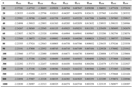
Based on these results, the values of some commonly used quantile points, are provided

for

n

=10, 20. . . 1000 in Appendix Tables A2–A11 at some representative values of

𝜌

.

The similar results can easily be obtained for any combination of

𝜌

and

n

. These

quantile points help determining the control limits and the power of the proposed

Pr

chart

to detect shifts in process of proportion of the defectives.

3. Parameters of the Proposed Chart

Finally, the control limits for the proposed control chart is given as

𝐿𝐶𝐿 = 𝑃̅

− 3𝜎

𝐶𝐿 = 𝑃̅

𝑈𝐶𝐿 = 𝑃̅

+ 3𝜎

By using results

𝐿𝐶𝐿 = 𝑃̅

− 3𝑐

𝜎̂

√𝑛

⁄

𝐶𝐿 = 𝑃̅

𝑈𝐶𝐿 = 𝑃̅

+ 3𝑐

𝜎̂

√𝑛

⁄

The use of 3-sigma limits is based on the symmetric assumption of the plotted statistic,

we will see that the distribution of Pr is not symmetric at least for small to moderate

values of n. Hence there is a need to develop the probability limit structure for the

proposed chart. Probability limits for the proposed chart can be computed by using

quantile points of the distribution of C.

Let α be the specified probability of making Type-I error, denoting α-quantile of the

distribution of C by

𝐶

. The probability limits based on Pr are given as:

𝐿𝐶𝐿 = 𝑃

with

𝑃

(𝑃

= 𝑃

) ≤∝

𝑈𝐶𝐿 = 𝑃

with

𝑃

(𝑃

= 𝑃

) ≥ 1 −∝

Where

∝=∝

+

∝

and

Pn

represents the cumulative distribution function for a given

value of

n

.

Now after simplification, we have the following results.

𝐿𝐶𝐿 = 𝑃

= 𝑃̅

+ 𝐶

𝜎̂

⁄

√𝑛

with

𝑃

(𝑐 = 𝑐

) ≤∝

We need to find the results of the following by using simulation method.

𝐿𝐶𝐿 = 𝑃̅

+ 𝐶

𝜎̂

⁄

√𝑛

𝐶𝐿 = 𝑃̅

𝑈𝐶𝐿 = 𝑃̅

+ 𝐶

𝜎̂

⁄

√𝑛

The values of

k

are provided in Appendix Table1 for

n

=10, 20, 100, 500, 1000.

Asymptotically,

C

is normally distributed, from Appendix Tables A2–A11.

4. Comparison

In this paper the performance of the

Pr

chart is compared with

P

(conventional Shewhart

attribute control chart) and

Q

chart for binomial data developed by Quesenberry (1991).

The efficiency of

Pr

chart as compared to

P

and

Q

chart has been examined using power

curves as a performance measure. Using their respective control structures, the power

curves for different combinations of

𝜌

have been constructed.

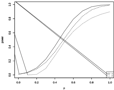
Figure 1: Power curves of Pr, P and Q charts for

𝜌

= 0.30

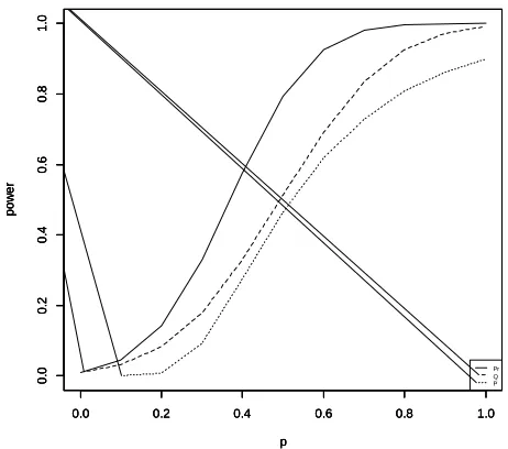
Figure 2: Power curves of Pr, P and Q charts for

𝜌

= 0.60

0.0 0.2 0.4 0.6 0.8 1.0

0. 0 0. 2 0. 4 0. 6 0. 8 1. 0 p po w er

0.0 0.2 0.4 0.6 0.8 1.0

0. 0 0. 2 0. 4 0. 6 0. 8 1. 0 p po w er

0.0 0.2 0.4 0.6 0.8 1.0

0. 0 0. 2 0. 4 0. 6 0. 8 1. 0 p po w er Pr Q P

0.0 0.2 0.4 0.6 0.8 1.0

0 .0 0 .2 0 .4 0 .6 0 .8 1 .0 p p o w e r

0.0 0.2 0.4 0.6 0.8 1.0

0 .0 0 .2 0 .4 0 .6 0 .8 1 .0 p p o w e r

0.0 0.2 0.4 0.6 0.8 1.0

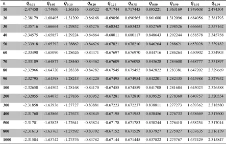
Figure 3: Power curves of Pr, P and Q charts for

𝜌

= 0.90

Figures 1-3 shown that the power curve of

Pr

chart is almost equally powerful as Q chart

and more powerful for

𝜌

= 0.30

, and more powerful then Q and P chart for

𝜌

=

0.60 𝑎𝑛𝑑 𝜌

= 0.90.

This show that the

Pr

chart has higher probability to signal shifts in process of

non-confirming items as compared to both

P

and

Q

chart.

5. Conclusion

The attribute control charts are particularly useful in the service industries and in

non-confirming quality improvement efforts. The classical application of

P

chart requires that

the parameters of the distribution are known. In many situations the true fraction

nonconforming,

P

, is unknown and need to be estimated. This study proposes an efficient

control chart, namely

Pr

chart, to monitor the process proportion or the non-confirming

items, based on proportion regression estimator. We derive the parameters of the

proposed chart. The performance of the proposed chart is compared with the classical

P

and

Q

charts using OC curves. It has been shown that Pr chart more efficient to the

P

and

Q

chart. The design of the

Pr

chart is established and is shown to be more efficient as

compared to the classical

P

chart and

Q

chart, particularly for bivariate data.

Acknowledgements

The authors are deeply thankful to editor and reviewers for their valuable suggestions to

improve the quality of this manuscript. This article was funded by the Deanship of

Scientific Research (DSR), King Abdulaziz University, Jeddah. The author, Muhammad

Aslam, therefore, acknowledge with thanks DSR technical and financial support.

0.0 0.2 0.4 0.6 0.8 1.0

0 .0 0 .2 0 .4 0 .6 0 .8 1 .0 p p o w e r

0.0 0.2 0.4 0.6 0.8 1.0

0 .0 0 .2 0 .4 0 .6 0 .8 1 .0 p p o w e r

0.0 0.2 0.4 0.6 0.8 1.0

6. References

1.

Acosta, M., Pignatiello JJ, Rao, B.V. (1999). A comparison of control charting

procedures for monitoring process dispersion

. IIE Trans

ition. 31,569–579.

2.

Das, A. K. (1982). On the use of auxiliary information in estimating proportions.

Journal of Indian Statistical Association

, 20, 99-108.

3.

Hillier, F. S. (1969).

𝑋̅

and

R

chart control limits based on a small number of

subgroups,

Journal of Quality Technology,

1, 17–26.

4.

Mehmood, R., Riaz, M., & Does, R. J. M. M. (2013). Control charts for location

based on different sampling schemes.

Journal of Applied Statistics

, 40(3),

483-494.

5.

Montgomery, D. C. (2003). "Introduction to Statistical Quality Control." 5th ed.,

John Wiley & Sons, New York, NY.

6.

Niaki, S. T. A., & Abbasi, B. (2007). On the monitoring of multi-attributes

high-quality production processes.

Metrika

,

66

(3), 373-388.

7.

Quesenberry, C.P. (1991). SPC Q charts for binomial parameter p: Short or long

runs.

Journal of Quality Technology,

23, 239-246.

8.

Riaz, M. (2008). Monitoring process mean level using auxiliary information.

Statistica Neerlandica, 62(4), 458–481.

9.

Riaz, Muhammad, Ahmad, S. Riaz, M., Abbasi, S. A. and Lin, Z. Y. (2014). On

Efficient Median Control Charting. Journal of the Chinese Institute of Engineers.

Journal of the Chinese Institute of Engineers

, 37,

358-375

10.

Ross, S. M. (1990). A course in simulations,

Macmillan Publishing Co. New

York

.

11.

Shewhart, W.A. (1924). Some applications of statistical methods to the analysis

of physical and engineering data.

Bell System Technical Journal,

3(1), 43-87.

12.

Shore, H (2000). General control charts for attributes. IIE Transactions 32, 1

149-1 149-160.

7. Appendix

Table 1: Control chart coefficient k of the Pr chart

Table 2: Quantile points of the distribution of Q (when

𝝆

= 𝟎. 𝟏

)

n 𝑸𝟎.𝟎𝟏 𝑸𝟎.𝟎𝟓 𝑸𝟎.𝟏𝟎 𝑸𝟎.𝟐𝟎 𝑸𝟎.𝟐𝟓 𝑸𝟎.𝟕𝟓 𝑸𝟎.𝟖𝟎 𝑸𝟎.𝟗𝟎 𝑸𝟎.𝟗𝟓 𝑸𝟎.𝟗𝟗

10 -2.47450 -1.74960 -1.36316 -0.89522 -0.71744 0.717445 0.895221 1.363169 1.749608 2.474504

20 -2.38179 -1.68405 -1.31209 -0.86168 -0.69056 0.690565 0.861680 1.312096 1.684056 2.381793

30 -2.35716 -1.66664 -1.29852 -0.85276 -0.68342 0.683423 0.852769 1.298526 1.666641 2.357162

40 -2.34575 -1.65857 -1.29224 -0.84864 -0.68011 0.680117 0.848643 1.292244 1.658578 2.345758

50 -2.33918 -1.65392 -1.28862 -0.84626 -0.67821 0.678210 0.846264 1.288621 1.653928 2.339182

60 -2.33490 -1.65090 -1.28626 -0.84471 -0.67697 0.676970 0.844716 1.286264 1.650902 2.334903

70 -2.33189 -1.64877 -1.28460 -0.84362 -0.67609 0.676098 0.843628 1.284608 1.648777 2.331897

80 -2.32966 -1.64720 -1.28338 -0.84282 -0.67545 0.675452 0.842822 1.283381 1.647202 2.329669

90 -2.32795 -1.64598 -1.28243 -0.84220 -0.67495 0.674954 0.842201 1.282435 1.645988 2.327952

100 -2.32658 -1.64502 -1.28168 -0.84170 -0.67455 0.674559 0.841708 1.281684 1.645023 2.326588

200 -2.32055 -1.64075 -1.27836 -0.83952 -0.67281 0.672810 0.839525 1.278360 1.640757 2.320554

300 -2.31858 -1.63936 -1.27727 -0.83881 -0.67223 0.672237 0.838811 1.277273 1.639362 2.318580

400 -2.31760 -1.63866 -1.27673 -0.83845 -0.67195 0.671953 0.838456 1.276733 1.638669 2.317600

500 -2.31701 -1.63825 -1.27641 -0.83824 -0.67178 0.671783 0.838244 1.276410 1.638254 2.317014

800 -2.31613 -1.63763 -1.27592 -0.83792 -0.67152 0.671529 0.837927 1.275927 1.637635 2.316139

1000 -2.31584 -1.63742 -1.27576 -0.83782 -0.67144 0.671445 0.837822 1.275767 1.637429 2.315847

n 0.1 0.2 0.3 0.4 0.5 0.6 0.7 0.8 0.9 0.99

10

1.064 1.047 1.019 0.979 0.925 0.855 0.763 0.641 0.466 0.151

20 1.024 1.008 0.981 0.943 0.891 0.823 0.735 0.617 0.449 0.145

30 1.013 0.997 0.971 0.933 0.881 0.815 0.727 0.611 0.448 0.143

40 1.008 0.992 0.966 0.928 0.877 0.810 0.724 0.608 0.443 0.142

50 1.006 0.990 0.964 0.926 0.875 0.808 0.721 0.606 0.441 0.142

60 1.004 0.988 0.962 0.924 0.873 0.806 0.720 0.605 0.439 0.142

70 1.002 0.987 0.961 0.923 0.872 0.805 0.719 0.604 0.439 0.142

80 1.001 0.986 0.960 0.922 0.871 0.805 0.719 0.603 0.439 0.141

90 1.000 0.985 0.959 0.922 0.870 0.804 0.718 0.603 0.438 0.141

100 1.000 0.984 0.958 0.921 0.870 0.804 0.717 0.603 0.438 0.141

500 0.996 0.981 0.953 0.917 0.866 0.800 0.714 0.600 0.436 0.141

Table 3: Quantile points of the distribution of Q (when

𝝆

= 𝟎. 𝟐

)

n 𝑸𝟎.𝟎𝟏 𝑸𝟎.𝟎𝟓 𝑸𝟎.𝟏𝟎 𝑸𝟎.𝟐𝟎 𝑸𝟎.𝟐𝟓 𝑸𝟎.𝟕𝟓 𝑸𝟎.𝟖𝟎 𝑸𝟎.𝟗𝟎 𝑸𝟎.𝟗𝟓 𝑸𝟎.𝟗𝟗

10 -2.43672 -1.72289 -1.34235 -0.88155 -0.70649 0.706491 0.881552 1.342356 1.722895 2.436723

20 -2.34542 -1.65834 -1.29206 -0.84852 -0.68002 0.680021 0.848523 1.292062 1.658344 2.345428

30 -2.32117 -1.64119 -1.27870 -0.83974 -0.67298 0.672989 0.839748 1.278701 1.641194 2.321172

40 -2.30994 -1.63325 -1.27251 -0.83568 -0.66973 0.669733 0.835686 1.272514 1.633254 2.309943

50 -2.30346 -1.62867 -1.26894 -0.83334 -0.66785 0.667855 0.833343 1.268947 1.628675 2.303467

60 -2.29925 -1.62569 -1.26662 -0.83181 -0.66663 0.666634 0.831819 1.266626 1.625696 2.299253

70 -2.29629 -1.62360 -1.26499 -0.83074 -0.66577 0.665775 0.830748 1.264995 1.623603 2.296293

80 -2.29409 -1.62205 -1.26378 -0.82995 -0.66513 0.665139 0.829954 1.263786 1.622052 2.294099

90 -2.29240 -1.62085 -1.26285 -0.82934 -0.66464 0.664649 0.829342 1.262855 1.620857 2.292408

100 -2.29106 -1.61990 -1.26211 -0.82885 -0.66426 0.664260 0.828856 1.262115 1.619907 2.291065

200 -2.28512 -1.61570 -1.25884 -0.82670 -0.66253 0.662537 0.826707 1.258842 1.615706 2.285124

300 -2.28318 -1.61433 -1.25777 -0.82600 -0.66197 0.661973 0.826004 1.257771 1.614332 2.283180

400 -2.28221 -1.61364 -1.25723 -0.82565 -0.66169 0.661694 0.825654 1.257239 1.613649 2.282215

500 -2.28163 -1.61324 -1.25692 -0.82544 -0.66152 0.661526 0.825446 1.256922 1.613241 2.281638

800 -2.28077 -1.61263 -1.25644 -0.82513 -0.66127 0.661276 0.825134 1.256446 1.612632 2.280776

1000 -2.28048 -1.61242 -1.25628 -0.82503 -0.66119 0.661193 0.825030 1.256289 1.612429 2.280489

Table 4: Quantile points of the distribution of Q (when

𝝆

= 𝟎. 𝟑

)

n 𝑸𝟎.𝟎𝟏 𝑸𝟎.𝟎𝟓 𝑸𝟎.𝟏𝟎 𝑸𝟎.𝟐𝟎 𝑸𝟎.𝟐𝟓 𝑸𝟎.𝟕𝟓 𝑸𝟎.𝟖𝟎 𝑸𝟎.𝟗𝟎 𝑸𝟎.𝟗𝟓 𝑸𝟎.𝟗𝟗

10 -2.37241 -1.67742 -1.30693 -0.85828 -0.68784 0.687847 0.858288 1.306931 1.677428 2.372419

20 -2.28353 -1.61458 -1.25796 -0.82613 -0.66207 0.662076 0.826131 1.257965 1.614581 2.283532

30 -2.25991 -1.59788 -1.24495 -0.81758 -0.65522 0.655229 0.817588 1.244956 1.597883 2.259917

40 -2.24898 -1.59015 -1.23893 -0.81363 -0.65205 0.652059 0.813632 1.238933 1.590153 2.248984

50 -2.24267 -1.58569 -1.23545 -0.81135 -0.65023 0.650231 0.811351 1.235459 1.585695 2.242679

60 -2.23857 -1.58279 -1.23320 -0.80986 -0.64904 0.649041 0.809867 1.233200 1.582794 2.238576

70 -2.23569 -1.58075 -1.23161 -0.80882 -0.64820 0.648206 0.808824 1.231612 1.580757 2.235694

80 -2.23355 -1.57924 -1.23043 -0.80805 -0.64758 0.647586 0.808052 1.230435 1.579246 2.233558

90 -2.23191 -1.57808 -1.22952 -0.80745 -0.64710 0.647109 0.807456 1.229528 1.578082 2.231912

100 -2.23060 -1.57715 -1.22880 -0.80698 -0.64673 0.646730 0.806983 1.228808 1.577158 2.230604

200 -2.22482 -1.57306 -1.22562 -0.80489 -0.64505 0.645053 0.804890 1.225621 1.573068 2.224820

300 -2.22292 -1.57173 -1.22457 -0.80420 -0.64450 0.644504 0.804206 1.224579 1.571730 2.222927

400 -2.22198 -1.57106 -1.22406 -0.80386 -0.64423 0.644232 0.803866 1.224061 1.571065 2.221988

500 -2.22142 -1.57066 -1.22375 -0.80366 -0.64406 0.644069 0.803662 1.223752 1.570668 2.221426

800 -2.22058 -1.57007 -1.22328 -0.80335 -0.64382 0.643825 0.803359 1.223289 1.570074 2.220586

Table 5: Quantile points of the distribution of Q (when

𝝆

= 𝟎. 𝟒

)

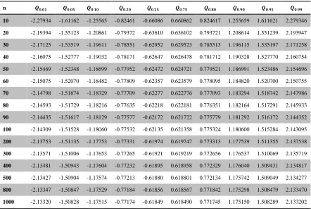
n 𝑸𝟎.𝟎𝟏 𝑸𝟎.𝟎𝟓 𝑸𝟎.𝟏𝟎 𝑸𝟎.𝟐𝟎 𝑸𝟎.𝟐𝟓 𝑸𝟎.𝟕𝟓 𝑸𝟎.𝟖𝟎 𝑸𝟎.𝟗𝟎 𝑸𝟎.𝟗𝟓 𝑸𝟎.𝟗𝟗

10 -2.27934 -1.61162 -1.25565 -0.82461 -0.66086 0.660862 0.824617 1.255659 1.611621 2.279346

20 -2.19394 -1.55123 -1.20861 -0.79372 -0.63610 0.636102 0.793721 1.208614 1.551239 2.193947

30 -2.17125 -1.53519 -1.19611 -0.78551 -0.62952 0.629523 0.785513 1.196115 1.535197 2.171258

40 -2.16075 -1.52777 -1.19032 -0.78171 -0.62647 0.626478 0.781712 1.190328 1.527770 2.160754

50 -2.15469 -1.52348 -1.18699 -0.77952 -0.62472 0.624721 0.779521 1.186991 1.523486 2.154696

60 -2.15075 -1.52070 -1.18482 -0.77809 -0.62357 0.623579 0.778095 1.184820 1.520700 2.150755

70 -2.14798 -1.51874 -1.18329 -0.77709 -0.62277 0.622776 0.777093 1.183294 1.518742 2.147986

80 -2.14593 -1.51729 -1.18216 -0.77635 -0.62218 0.622181 0.776351 1.182164 1.517291 2.145933

90 -2.14435 -1.51617 -1.18129 -0.77577 -0.62172 0.621722 0.775779 1.181292 1.516172 2.144352

100 -2.14309 -1.51528 -1.18060 -0.77532 -0.62135 0.621358 0.775324 1.180600 1.515284 2.143095

200 -2.13753 -1.51135 -1.17753 -0.77331 -0.61974 0.619747 0.773313 1.177539 1.511355 2.137538

300 -2.13571 -1.51006 -1.17653 -0.77265 -0.61921 0.619219 0.772656 1.176537 1.510069 2.135719

400 -2.13481 -1.50943 -1.17604 -0.77232 -0.61895 0.618958 0.772329 1.176040 1.509431 2.134817

500 -2.13427 -1.50904 -1.17574 -0.77213 -0.61880 0.618801 0.772134 1.175742 1.509049 2.134277

800 -2.13347 -1.50847 -1.17529 -0.77184 -0.61856 0.618567 0.771842 1.175298 1.508479 2.133470

1000 -2.13320 -1.50828 -1.17515 -0.77174 -0.61849 0.618490 0.771745 1.175150 1.508289 2.133202

Table 6: Quantile points of the distribution of Q (when

𝝆

= 𝟎. 𝟓

)

n 𝑸𝟎.𝟎𝟏 𝑸𝟎.𝟎𝟓 𝑸𝟎.𝟏𝟎 𝑸𝟎.𝟐𝟎 𝑸𝟎.𝟐𝟓 𝑸𝟎.𝟕𝟓 𝑸𝟎.𝟖𝟎 𝑸𝟎.𝟗𝟎 𝑸𝟎.𝟗𝟓 𝑸𝟎.𝟗𝟗

10 -2.15378 -1.52283 -1.18648 -0.77918 -0.62445 0.624456 0.779189 1.186486 1.522839 2.153780

20 -2.07308 -1.46578 -1.14203 -0.74999 -0.60105 0.601059 0.749996 1.142033 1.465783 2.073085

30 -2.05164 -1.45062 -1.13022 -0.74224 -0.59484 0.594844 0.742240 1.130222 1.450625 2.051646

40 -2.04172 -1.44360 -1.12475 -0.73864 -0.59196 0.591966 0.738649 1.124754 1.443606 2.041720

50 -2.03599 -1.43955 -1.12160 -0.73657 -0.59030 0.590306 0.736578 1.121601 1.439559 2.035996

60 -2.03227 -1.43692 -1.11954 -0.73523 -0.58922 0.589226 0.735231 1.119549 1.436926 2.032272

70 -2.02965 -1.43507 -1.11810 -0.73428 -0.58846 0.588468 0.734284 1.118108 1.435076 2.029656

80 -2.02771 -1.43370 -1.11704 -0.73358 -0.58790 0.587906 0.733583 1.117040 1.433705 2.027716

90 -2.02622 -1.43264 -1.11621 -0.73304 -0.58747 0.587472 0.733042 1.116216 1.432648 2.026222

100 -2.02503 -1.43180 -1.115562 -0.73261 -0.58712 0.587128 0.732612 1.115562 1.431809 2.025035

200 -2.01978 -1.42809 -1.112670 -0.73071 -0.58560 0.585605 0.730712 1.112670 1.428096 2.019783

300 -2.01806 -1.42688 -1.111723 -0.73009 -0.58510 0.585107 0.730091 1.111723 1.426881 2.018065

400 -2.01721 -1.42627 -1.111253 -0.72978 -0.58486 0.584860 0.729782 1.111253 1.426278 2.017212

500 -2.01670 -1.42591 -1.110972 -0.72959 -0.58471 0.584712 0.729598 1.110972 1.425917 2.016702

800 -2.01594 -1.42537 -1.110552 -0.72932 -0.58449 0.584491 0.729322 1.110552 1.425378 2.015940

Table 7: Quantile points of the distribution of Q (when

𝝆

= 𝟎. 𝟔

)

n 𝑸𝟎.𝟎𝟏 𝑸𝟎.𝟎𝟓 𝑸𝟎.𝟏𝟎 𝑸𝟎.𝟐𝟎 𝑸𝟎.𝟐𝟓 𝑸𝟎.𝟕𝟓 𝑸𝟎.𝟖𝟎 𝑸𝟎.𝟗𝟎 𝑸𝟎.𝟗𝟓 𝑸𝟎.𝟗𝟗

10 -1.98957 -1.40673 -1.09602 -0.71978 -0.57684 0.576847 0.719784 1.096029 1.406738 1.989576

20 -1.91503 -1.35403 -1.05496 -0.69281 -0.55523 0.555235 0.692816 1.054965 1.354032 1.915034

30 -1.89522 -1.34003 -1.04405 -0.68565 -0.54949 0.549493 0.685652 1.044055 1.340030 1.895229

40 -1.88606 -1.33354 -1.04405 -0.68233 -0.54683 0.546835 0.682334 1.044055 1.333547 1.886060

50 -1.88077 -1.32980 -1.03900 -0.68042 -0.54530 0.545301 0.680422 1.039003 1.329808 1.880773

60 -1.87733 -1.32737 -1.03609 -0.67917 -0.54430 0.544304 0.679177 1.036091 1.327376 1.877333

70 -1.87491 -1.32566 -1.03419 -0.67830 -0.54360 0.543603 0.678303 1.034195 1.325667 1.874916

80 -1.87312 -1.32440 -1.03286 -0.67765 -0.54308 0.543084 0.677654 1.032864 1.324400 1.873124

90 -1.87174 -1.32342 -1.03187 -0.67715 -0.54268 0.542684 0.677155 1.031877 1.323424 1.871744

100 -1.87064 -1.32264 -1.031117 -0.67675 -0.54236 0.542366 0.676758 1.031117 1.322648 1.870647

200 -1.86579 -1.31921 -1.03051 -0.67500 -0.54095 0.540959 0.675003 1.030512 1.319218 1.865796

300 -1.86420 -1.31809 -1.02784 -0.67442 -0.54049 0.540499 0.674429 1.027840 1.318096 1.864209

400 -1.86342 -1.31753 -1.02696 -0.67414 -0.54027 0.540271 0.674144 1.026966 1.317539 1.863421

500 -1.86295 -1.31720 -1.02653 -0.67397 -0.54013 0.540134 0.673974 1.026532 1.317206 1.862950

800 -1.86224 -1.31670 -1.02627 -0.67371 -0.53993 0.539930 0.673719 1.026272 1.316708 1.862245

1000 -1.86201 -1.31654 -1.02588 -0.67363 -0.53986 0.539862 0.673634 1.025884 1.316543 1.862011

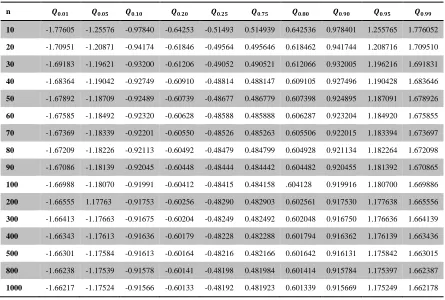
Table 8: Quantile points of the distribution of Q (when

𝝆

= 𝟎. 𝟕

)

n 𝑸𝟎.𝟎𝟏 𝑸𝟎.𝟎𝟓 𝑸𝟎.𝟏𝟎 𝑸𝟎.𝟐𝟎 𝑸𝟎.𝟐𝟓 𝑸𝟎.𝟕𝟓 𝑸𝟎.𝟖𝟎 𝑸𝟎.𝟗𝟎 𝑸𝟎.𝟗𝟓 𝑸𝟎.𝟗𝟗

10 -1.77605 -1.25576 -0.97840 -0.64253 -0.51493 0.514939 0.642536 0.978401 1.255765 1.776052

20 -1.70951 -1.20871 -0.94174 -0.61846 -0.49564 0.495646 0.618462 0.941744 1.208716 1.709510

30 -1.69183 -1.19621 -0.93200 -0.61206 -0.49052 0.490521 0.612066 0.932005 1.196216 1.691831

40 -1.68364 -1.19042 -0.92749 -0.60910 -0.48814 0.488147 0.609105 0.927496 1.190428 1.683646

50 -1.67892 -1.18709 -0.92489 -0.60739 -0.48677 0.486779 0.607398 0.924895 1.187091 1.678926

60 -1.67585 -1.18492 -0.92320 -0.60628 -0.48588 0.485888 0.606287 0.923204 1.184920 1.675855

70 -1.67369 -1.18339 -0.92201 -0.60550 -0.48526 0.485263 0.605506 0.922015 1.183394 1.673697

80 -1.67209 -1.18226 -0.92113 -0.60492 -0.48479 0.484799 0.604928 0.921134 1.182264 1.672098

90 -1.67086 -1.18139 -0.92045 -0.60448 -0.48444 0.484442 0.604482 0.920455 1.181392 1.670865

100 -1.66988 -1.18070 -0.91991 -0.60412 -0.48415 0.484158 .604128 0.919916 1.180700 1.669886

200 -1.66555 1.17763 -0.91753 -0.60256 -0.48290 0.482903 0.602561 0.917530 1.177638 1.665556

300 -1.66413 -1.17663 -0.91675 -0.60204 -0.48249 0.482492 0.602048 0.916750 1.176636 1.664139

400 -1.66343 -1.17613 -0.91636 -0.60179 -0.48228 0.482288 0.601794 0.916362 1.176139 1.663436

500 -1.66301 -1.17584 -0.91613 -0.60164 -0.48216 0.482166 0.601642 0.916131 1.175842 1.663015

800 -1.66238 -1.17539 -0.91578 -0.60141 -0.48198 0.481984 0.601414 0.915784 1.175397 1.662387

Table 9: Quantile points of the distribution of Q (when

𝝆

== 𝟎. 𝟖

)

n 𝑸𝟎.𝟎𝟏 𝑸𝟎.𝟎𝟓 𝑸𝟎.𝟏𝟎 𝑸𝟎.𝟐𝟎 𝑸𝟎.𝟐𝟓 𝑸𝟎.𝟕𝟓 𝑸𝟎.𝟖𝟎 𝑸𝟎.𝟗𝟎 𝑸𝟎.𝟗𝟓 𝑸𝟎.𝟗𝟗

10 -1.49218 -1.05505 -0.82202 -0.53983 -0.43263 0.432635 0.539838 0.822021 1.055053 1.492182

20 -1.43627 -1.01552 -0.79122 -0.51961 -0.41642 0.416426 0.519612 0.791223 1.015524 1.436275

30 -1.42142 -1.00502 -0.78304 -0.51423 -0.41212 0.412120 0.514239 0.783040 1.005022 1.421422

40 -1.41454 -1.00015 -0.77925 -0.51175 -0.41012 0.410126 0.511751 0.779252 1.000159 1.414545

50 -1.41058 -0.99735 -0.77706 -0.51031 -0.40897 0.408976 0.510316 0.777068 0.997356 1.410580

60 -1.40799 -0.99553 -0.77564 -0.50938 -0.40822 0.408228 0.509383 0.775646 0.995531 1.407999

70 -1.40618 -0.99424 -0.77464 -0.50872 -0.40770 0.407702 0.508727 0.774648 0.994249 1.406187

80 -1.40484 -0.99330 -0.77390 -0.50824 -0.40731 0.407313 0.508241 0.773907 0.993300 1.404843

90 -1.40380 -0.99256 -0.77333 -0.50786 -0.40701 0.407013 0.507866 0.773337 0.992567 1.403808

100 -1.40298 -0.99198 -0.77288 -0.50756 -0.40677 0.406774 0.507569 0.772884 0.991986 1.402985

200 -1.39934 -0.98941 -0.77088 -0.50625 -0.40571 0.405719 0.506252 0.770880 0.989413 1.399347

300 -1.39815 -0.98857 -0.77022 -0.50582 -0.40537 0.405374 0.505822 0.770224 0.988572 1.398157

400 -1.39756 -0.98815 -0.76989 -0.50560 -0.40520 0.405203 0.505608 0.769898 0.988154 1.397566

500 -1.39721 -0.98790 -0.76970 -0.50548 -0.40510 0.405100 0.505480 0.769704 0.987904 1.397212

800 -1.39668 -0.98753 -0.76941 -0.50528 -0.40494 0.404947 0.505289 0.769413 0.987531 1.396684

1000 -1.39650 -0.98740 -0.76931 -0.50522 -0.40489 0.404896 0.505225 0.769316 0.987407 1.396509

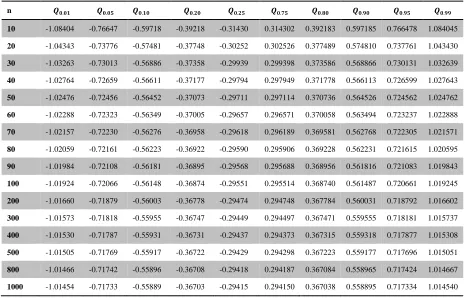
Table 10: Quantile points of the distribution of Q (when

𝝆

= 𝟎. 𝟗

)

n 𝑸𝟎.𝟎𝟏 𝑸𝟎.𝟎𝟓 𝑸𝟎.𝟏𝟎 𝑸𝟎.𝟐𝟎 𝑸𝟎.𝟐𝟓 𝑸𝟎.𝟕𝟓 𝑸𝟎.𝟖𝟎 𝑸𝟎.𝟗𝟎 𝑸𝟎.𝟗𝟓 𝑸𝟎.𝟗𝟗

10 -1.08404 -0.76647 -0.59718 -0.39218 -0.31430 0.314302 0.392183 0.597185 0.766478 1.084045

20 -1.04343 -0.73776 -0.57481 -0.37748 -0.30252 0.302526 0.377489 0.574810 0.737761 1.043430

30 -1.03263 -0.73013 -0.56886 -0.37358 -0.29939 0.299398 0.373586 0.568866 0.730131 1.032639

40 -1.02764 -0.72659 -0.56611 -0.37177 -0.29794 0.297949 0.371778 0.566113 0.726599 1.027643

50 -1.02476 -0.72456 -0.56452 -0.37073 -0.29711 0.297114 0.370736 0.564526 0.724562 1.024762

60 -1.02288 -0.72323 -0.56349 -0.37005 -0.29657 0.296571 0.370058 0.563494 0.723237 1.022888

70 -1.02157 -0.72230 -0.56276 -0.36958 -0.29618 0.296189 0.369581 0.562768 0.722305 1.021571

80 -1.02059 -0.72161 -0.56223 -0.36922 -0.29590 0.295906 0.369228 0.562231 0.721615 1.020595

90 -1.01984 -0.72108 -0.56181 -0.36895 -0.29568 0.295688 0.368956 0.561816 0.721083 1.019843

100 -1.01924 -0.72066 -0.56148 -0.36874 -0.29551 0.295514 0.368740 0.561487 0.720661 1.019245

200 -1.01660 -0.71879 -0.56003 -0.36778 -0.29474 0.294748 0.367784 0.560031 0.718792 1.016602

300 -1.01573 -0.71818 -0.55955 -0.36747 -0.29449 0.294497 0.367471 0.559555 0.718181 1.015737

400 -1.01530 -0.71787 -0.55931 -0.36731 -0.29437 0.294373 0.367315 0.559318 0.717877 1.015308

500 -1.01505 -0.71769 -0.55917 -0.36722 -0.29429 0.294298 0.367223 0.559177 0.717696 1.015051

800 -1.01466 -0.71742 -0.55896 -0.36708 -0.29418 0.294187 0.367084 0.558965 0.717424 1.014667

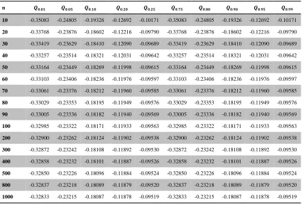
Table 11: Quantile points of the distribution of Q (when

𝝆

= 𝟎. 𝟗𝟗

)

n 𝑸𝟎.𝟎𝟏 𝑸𝟎.𝟎𝟓 𝑸𝟎.𝟏𝟎 𝑸𝟎.𝟐𝟎 𝑸𝟎.𝟐𝟓 𝑸𝟎.𝟕𝟓 𝑸𝟎.𝟖𝟎 𝑸𝟎.𝟗𝟎 𝑸𝟎.𝟗𝟓 𝑸𝟎.𝟗𝟗

10 -0.35083 -0.24805 -0.19326 -0.12692 -0.10171 -0.35083 -0.24805 -0.19326 -0.12692 -0.10171

20 -0.33768 -0.23876 -0.18602 -0.12216 -0.09790 -0.33768 -0.23876 -0.18602 -0.12216 -0.09790

30 -0.33419 -0.23629 -0.18410 -0.12090 -0.09689 -0.33419 -0.23629 -0.18410 -0.12090 -0.09689

40 -0.33257 -0.23514 -0.18321 -0.12031 -0.09642 -0.33257 -0.23514 -0.18321 -0.12031 -0.09642

50 -0.33164 -0.23449 -0.18269 -0.11998 -0.09615 -0.33164 -0.23449 -0.18269 -0.11998 -0.09615

60 -0.33103 -0.23406 -0.18236 -0.11976 -0.09597 -0.33103 -0.23406 -0.18236 -0.11976 -0.09597

70 -0.33061 -0.23376 -0.18212 -0.11960 -0.09585 -0.33061 -0.23376 -0.18212 -0.11960 -0.09585

80 -0.33029 -0.23353 -0.18195 -0.11949 -0.09576 -0.33029 -0.23353 -0.18195 -0.11949 -0.09576

90 -0.33005 -0.23336 -0.18182 -0.11940 -0.09569 -0.33005 -0.23336 -0.18182 -0.11940 -0.09569

100 -0.32985 -0.23322 -0.18171 -0.11933 -0.09563 -0.32985 -0.23322 -0.18171 -0.11933 -0.09563

200 -0.32900 -0.23262 -0.18124 -0.11902 -0.09538 -0.32900 -0.23262 -0.18124 -0.11902 -0.09538

300 -0.32872 -0.23242 -0.18108 -0.11892 -0.09530 -0.32872 -0.23242 -0.18108 -0.11892 -0.09530

400 -0.32858 -0.23232 -0.18101 -0.11887 -0.09526 -0.32858 -0.23232 -0.18101 -0.11887 -0.09526

500 -0.32850 -0.23226 -0.18096 -0.11884 -0.09524 -0.32850 -0.23226 -0.18096 -0.11884 -0.09524

800 -0.32837 -0.23218 -0.18089 -0.11879 -0.09520 -0.32837 -0.23218 -0.18089 -0.11879 -0.09520