https://doi.org/10.5194/esd-8-889-2017
© Author(s) 2017. This work is distributed under the Creative Commons Attribution 3.0 License.
A method to preserve trends in quantile mapping bias
correction of climate modeled temperature
Manolis G. Grillakis1, Aristeidis G. Koutroulis1, Ioannis N. Daliakopoulos1, and Ioannis K. Tsanis1,2 1Technical University of Crete, School of Environmental Engineering, Chania, Greece
2McMaster University, Department of Civil Engineering, Hamilton, ON, Canada
Correspondence to:Manolis G. Grillakis ([email protected])
Received: 30 May 2017 – Discussion started: 7 June 2017
Revised: 30 August 2017 – Accepted: 15 September 2017 – Published: 28 September 2017
Abstract. Bias correction of climate variables is a standard practice in climate change impact (CCI) studies. Various methodologies have been developed within the framework of quantile mapping. However, it is well known that quantile mapping may significantly modify the long-term statistics due to the time dependency of the temperature bias. Here, a method to overcome this issue without compromising the day-to-day correction statis-tics is presented. The methodology separates the modeled temperature signal into a normalized and a residual component relative to the modeled reference period climatology, in order to adjust the biases only for the former and preserve the signal of the later. The results show that this method allows for the preservation of the originally modeled long-term signal in the mean, the standard deviation and higher and lower percentiles of temperature. To illustrate the improvements, the methodology is tested on daily time series obtained from five Euro CORDEX regional climate models (RCMs).
1 Introduction
Climate model output provides the primary source of infor-mation used to quantify the effect of the foreseen anthro-pogenic climate change on natural systems. One of the most common and technically sound practices in climate change impact (CCI) studies is to calibrate impact models using the most suitable observational data and then to replace them with the climate model data in order to assess the effect of potential changes in the climate regime. Often, raw climate model data cannot be used in CCI models due to the presence of biases in the representation of regional climate (Chris-tensen et al., 2008; Haerter et al., 2011). In fact, hydrolog-ical CCI studies outcome have been reported to become un-realistic without a prior adjustment of climate forcing biases (Hagemann et al., 2013; Hansen et al., 2006; Harding et al., 2014; Sharma et al., 2007). Papadimitriou et al. (2017) quan-tified the effect of the bias in seven forcing parameters on the resulting runoff of a land surface model, emphasizing the necessity of bias adjustments beyond the precipitation and temperature parameters. These biases are attributed to a number of reasons such as the imperfect representation of
run using observational data is likely to be reproduced by the adjusted data. The good performance of statistical bias cor-rection methods in the reference period is well documented (Grillakis et al., 2011, 2013; Ines and Hansen, 2006; Pa-padimitriou et al., 2015). The procedure, however, overlooks the time dependency of the distribution and hence the un-equal effect of the TF to the varying over time CDF. An in-dicative example is presented in Fig. 1, where modeled tem-perature data have a mean bias of 2.49◦C in the reference period (Fig. 1a) relative to the observations. This mean bias is expressed by the average horizontal distance between the TF and the bisector of the central plot. The left histogram il-lustrates the reference period modeled data for 1981–2010. The histogram at the bottom is derived from observational data. The histogram on the right is derived from a moving 30-year period between 1981 and 2098. The rightmost his-togram shows the difference between the reference period and the moving 30-year period. The red mark shows the the-oretical change in the average correction applied by the TF, due to the changes in the projected temperature histogram. Hence, the average correction applied for the period 2068– 2097 reaches 3.85◦C, significantly higher than the reference period’s bias (Fig. 1b). The time-dependency of the correc-tion magnitude introduces a long-term signal distorcorrec-tion in the corrected data. In the quantile-mapping-based correction methodologies in which the TF distance from the bisector is variable, this effect is unavoidable. Nevertheless, in cases where the TF retains a relatively constant distance to the bi-sector (i.e., parallel to the bibi-sector), the trend of the corrected data remains similar to the raw model data regardless of the temporal change in the model data histogram.
Based on the previous example, the time extrapolation of the TF is regarded as a leap of faith that may lead to a false certainty about the robustness of the adjusted pro-jection. This may significantly change the original modeled long-term trend or other higher moments of the climate vari-able statistics that eventually change the long-term signal of the climate variable. In their work on distribution-based scaling (DBS) bias correction, Olsson et al. (2015) showed that their methodology might alter the long-term tempera-ture trends, attributing the phenomenon in the severity of the biases in the mean or the standard deviation between the un-corrected temperatures and the observations. Maraun (2016) discusses whether the change in the trend is a desired fea-ture of bias correction, concluding that it is case-specific and depends on the skillfulness of the climate model to simulate the correct long-term signal. In the case of CCI studies, this implies that climate model data are assessed for their skill to well represent the trend, which is not a common prac-tice. A possible but indirect solution to this is described in Maurer and Pierce (2014), who study the change in precipi-tation trend over an ensemble of atmospheric general circu-lation model (AGCM). They conclude that, while individual quantile-mapping-corrected AGCM data may significantly modify the signal of change, a relatively large ensemble
es-Figure 1.The transfer function (TF – heavy black line) between observed (bottom histograms) and modeled (histograms on the left) for the reference period (1981–2010) is used to adjust bias of a 30-year moving window from 1981–2010 to 2068–2097. The rightmost plot shows the residual histogram after bias correction. The change in the average correction (red mark) on the TF in comparison to the reference period mean correction (square) is shown. The animated version provided in the Supplement shows the temporal evolution of the bias as the 30-year time window moves on the projection data. Data were obtained from ICHEC-EC-EARTH r12i1p1 SMHI-RCA4_v1 RCM of Euro-CORDEX experi-ment (0.11◦resolution) simulation under the representative concen-tration pathway of RCP85, for the location Chania International Air-port (long=24.08, lat=35.54). Observational data were obtained from the E-OBS v14 dataset (Haylock et al., 2008) of 0.25◦spatial resolution.
values, indicating that specific correction values are attached to each temperature anomaly, while it also has the drawback that the edges of the distribution are not corrected adequately. A similar approach that is additive for temperature and mul-tiplicative for precipitation was also followed by Pierce et al. (2015). Bürger et al. (2013) and Cannon et al. (2015) test the de-trending of the data prior to their quantile mapping correction, figuring that the removal of the trends prior to the quantile mapping and their reintroduction after the correction tends without absolutely maintaining the long-term trend.
In this study, we present a methodology to conserve the long-term statistics such as trend and variability of the cli-mate model data in quantile mapping. The methodology con-siders the separation of the temperature signal relative to the raw data reference period, producing a normalized and a residuals data stream. The separation is performed on an annual basis. The residuals include the gradual changes in the signal and the year-to-year fluctuations in the distribution of the temperature. The quantile mapping bias correction is then applied to the normalized daily temperature. Finally, the residual components are merged to the bias-corrected time series to form the corrected time series. The idea of identi-fying and using two different timescales in bias correction of temperature was introduced in Haerter et al. (2011), who present a method to separate the different timescales and ap-ply a correction to each one. The methodology presented here is tested along with a generalized version of the multi-segment statistical bias correction (MSBC) quantile mapping methodology (Grillakis et al., 2013). The methodology takes the form of a pre- and post-processing module that can be ap-plied along with different statistical bias correction method-ologies. The two-step procedure is examined for its ability to remove the daily biases with simultaneous preservation of the long-term statistics. The procedure is compared to the simple quantile mapping and a quantile mapping in combi-nation with a simpler trend preservation procedure.
2 Methods
2.1 Residual separation
The statistical difference of each individual year’s simulated data, compared to the average reference period simulated data is identified as residuals. These are estimated between the CDF of each year’s modeled climate data and the CDF of the entire reference period of the model data. LetSR be the reference period model data andSi the climate data for yeari, then the normalized dataSiNfor yeariare estimated by transferring each year’s data onto the average reference period CDF through a transfer function TFSi estimated an-nually. This can be formulated as Eq. (1).
SiN=TF−S1
R TFSi(Si)
(1)
The difference between the original model data Si and the normalized dataSiNis the residual componentsSiDof the time
series (Eq. 2).
SiD=Si−SiN (2)
The original model dataSican be reproduced by adding back the residualsSiD to the normalized data SiN. After the sep-aration, the normalized climate model data are statistically bias-corrected following a suitable methodology. The resid-uals are preserved in order to be later added back to the bias-corrected time series. We refer to the described method as a normalization module (NM) to hereafter lighten the nomen-clature of the paper. The normalization procedure is per-formed on annual basis, as this consists of an obvious pe-riodicity to use in the case of temperature, even if it is not so well defined in the tropics. The underlying assumption of the NM procedure is that it considers no major changes in the reference period data, a notion that can hardly fall short due to the usually short length of the reference period.
2.2 Bias correction
Here, the NM is applied along with a modification of the MSBC algorithm that is presented in Grillakis et al. (2013). This methodology follows the principles of quantile mapping correction techniques and was originally designed and tested for GCM precipitation adjustment. The method partitions the CDF data into discrete segments and an individual quantile mapping correction is applied to each segment, achieving a better-fitted transfer function. Here the methodology is mod-ified to use linear functions instead of the gamma functions used in the original methodology, in order to facilitate po-tential negative temperature values but also as a known tech-nique in quantile mapping, as it has also been used elsewhere (Themeßl et al., 2011). An indicative example is shown in Fig. 2, where the CDFs are split into discrete segments and linear functions are fit to each of them. In Fig. 2,p symbol-izes the cumulative probability andsis the slope of the linear function. Then the corrected temperature for each tempera-ture value of the specific segment is estimated as in Eq. (3).
Tcorrn =sobsn · Tn
raw−brawn sn
raw
+bnobs (3)
Figure 2.MSBC methodology on temperature correction using linear functions (borrowed from Grillakis et al., 2013; modified) in one of the data segments.
2016). As the MSBC methodology belongs to the parametric quantile mapping techniques, it shares their advantages and drawbacks. A comprehensive shakedown of advantages and disadvantages of quantile mapping in comparison to other methods can be found in Maraun et al. (2010) and Themeßl et al. (2011). A step-by-step example of the multisegment correction procedure is provided in Appendix A of Grillakis et al. (2013).
2.3 Validation of the results
The Klemes (1986) split sample test methodology was adopted for verification. Split sample is the most common type of test used for the validation of model efficiency. The methodology considers two periods of calibration and valida-tion between the observed and modeled data. The first period is used for the calibration, while the second period is used as a pseudo-future period in which the adjusted data are as-sessed against the observations. A drawback of the split sam-ple test in bias correction validation operations is that the re-maining bias of the validation period is a function of the bias correction methodology deficiency and the model deficiency itself to describe the validation period’s climate, in aspects that are not intended to be bias-corrected. That said, a skill-ful bias correction method should deal well in that context, as model “democracy” (Knutti, 2010), i.e., the assumption that all model projections are equally possible, is common in CCI studies in which little attention is given to the model selection.
3 Case study area and data
To examine the effect of NM on the bias correction on a time series, the Hadley Centre Central England Tempera-ture (HadCET – Parker et al., 1992) observational dataset was considered to adjust the simulated output from the earth system model MIROC-ESM-CHEM (Hasumi and Emori, 2004) historical emissions run between 1850 and 2005 for central England. This particular case study was chosen due to the large observational record (the longest instrumental record of temperature in the world) that is available for cen-tral England, i.e., the triangular area of the United King-dom enclosed by Lancashire, London and Bristol. Discussion about dataset-related uncertainties can be found in Parker et al. (1992) and Parker and Horton (2005). In the specific application and in order to resemble a typical CCI study, data between 1850 and 1899 serve as the calibration pe-riod, while the rest of the data between 1900 and 2005 are used as the pseudo-future period for the validation. Finally, the bias correction results of the two procedures, with (BC-NM) and without (BC) the normalization module, were com-pared against the validation period observations. An addi-tional comparison was also performed to a less complicated trend preservation procedure, inspired by Bürger et al. (2013) and Cannon et al. (2015). This procedure considers the de-trending of the raw data using a 5-year moving average temperature. The detrended data are corrected using the BC methodology, while the trend is additively put back into the time series after the correction, similarly to the NM. We re-fer to this as BC-TREND. This comparison is used to bench-mark the BC-NM towards a simpler quantile mapping that also approaches the trend preservation.
Table 1.RCMs used in this experiment.
# {GCM}_{realization}_{RCM} 1 CNRM-CM5_r1i1p1_SMHI-RCA4_v1 2 EC-EARTH_r12i1p1_SMHI-RCA4_v1 3 EC-EARTH_r3i1p1_DMI-HIRHAM5_v1 4 IPSL-CM5A-MR_r1i1p1_SMHI-RCA4_v1
RCA4_v1RCA4_v1RCA4_v1
5 MPI-ESM-LR_r1i1p1_SMHI-RCA4_v1
the efficiency of the two procedures on a pan-European scale. In order to scale up the split sample test, thek-fold cross val-idation test (Geisser, 1993) is employed. The procedure has been proposed for evaluating the performance of bias correc-tion procedures in Maraun (2016). In thek-fold cross vali-dation test, the data are partitioned intokequal sized folds. Of the k folds, one subsample is retained each time as the validation data for testing the model, and the remainingk−1 subsamples are used as calibration data. In a final test, the procedures are applied on a long-term transient climate pro-jection experiment to assess their effect in the long-term at-tributes of the temperature in a European-scale application.
Temperature data from the European division of the Co-ordinated Regional Downscaling Experiment (CORDEX), openly available through the Earth System Grid Federation (ESGF), are considered. Additional information about the Euro CORDEX domain can be found on the CORDEX web page (http://wcrp-cordex.ipsl.jussieu.fr/). Data from five re-gional climate models (RCMs) (Table 1) with 0.44◦ spa-tial resolution and daily time step between 1951 and 2100 are used. The projection data are considered under Repre-sentative Concentration Pathway (RCP) 8.5, which projects an 8.5 W m−2 average increase in the radiative forcing un-til 2100. The European domain CORDEX simulations have been evaluated for their performance in previous studies (Kotlarski et al., 2014; Prein et al., 2015). The EOBSv12 temperature data were used (Haylock et al., 2008). Discus-sion about the applicability of EOBS to compare tempera-ture of RCMs control climate simulations can be found in Kyselý and Plavcová (2010). Figure 3 shows the 1951–2005 daily temperature average and standard deviation for the five RCMs of Table 1. The RCMs’ mean bias ranges between about−2 and 1◦C relative to the EOBS dataset (individual models data are included to the ESM). The positive mean bias in all RCMs is mainly seen in eastern Europe, while the same areas exhibit negative bias in standard deviation. Some of the bias may, however, be attributed to the ability of the observational dataset to represent the true temperature (Hof-stra et al., 2010).
For the k-fold cross validation, the RCM data between 1951 and 2010 are split into six 10-year sections, compris-ing a 6-fold, five-RCM-ensemble experiment of Fig. 4. Each section is validated once by using the remaining five sections
Figure 3.Mean temperature (upper) and standard deviation (lower) for EOBS, RCM ensemble (ENS) and for their difference (model – obs) (DIFF) for the reference period 1951–2005.
Figure 4.The 6-fold cross validation scheme with the calibration (C) and the validation (V) periods of each fold. Each experiment (Exp) was replicated for all five RCMs.
for the calibration. A total of 30 tests are conducted using each procedure.
For the transient experiment, the RCM data between 1951 and 2100 are considered, using the 1951–2010 as calibration to correct the 1951–2100 data.
4 Results
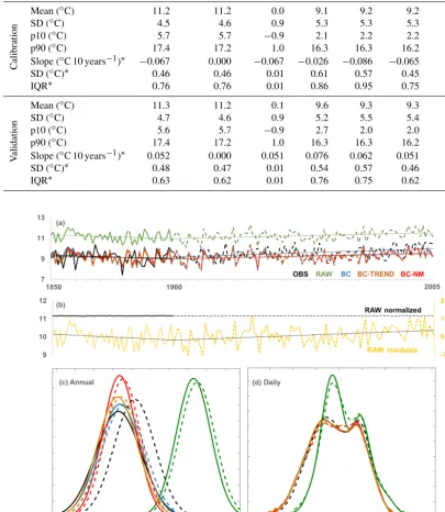
Table 2.Statistical properties of the calibration and the validation periods for the two bias correction procedures. Variables denoted with∗ are estimated on annual aggregates. SD stands for standard deviation, pnfor thenth quantile and IQR for the interquartile range.
Parameter RAW Normalized Residuals OBS BC BC-NM BCTREND
Calibration
Mean (◦C) 11.2 11.2 0.0 9.1 9.2 9.2 9.1 SD (◦C) 4.5 4.6 0.9 5.3 5.3 5.3 5.3 p10 (◦C) 5.7 5.7 −0.9 2.1 2.2 2.2 2.1 p90 (◦C) 17.4 17.2 1.0 16.3 16.3 16.2 16.2 Slope (◦C 10 years−1)∗ −0.067 0.000 −0.067 −0.026 −0.086 −0.065 −0.061 SD (◦C)∗ 0.46 0.46 0.01 0.61 0.57 0.45 0.53 IQR∗ 0.76 0.76 0.01 0.86 0.95 0.75 0.94
V
alidation
Mean (◦C) 11.3 11.2 0.1 9.6 9.3 9.3 9.2 SD (◦C) 4.7 4.6 0.9 5.2 5.5 5.4 5.5 p10 (◦C) 5.6 5.7 −0.9 2.7 2.0 2.0 1.9 p90 (◦C) 17.4 17.2 1.0 16.3 16.3 16.2 16.2 Slope (◦C 10 years−1)∗ 0.052 0.000 0.051 0.076 0.062 0.051 0.044 SD (◦C)∗ 0.48 0.47 0.01 0.54 0.57 0.46 0.53 IQR∗ 0.63 0.62 0.01 0.76 0.75 0.62 0.68
Figure 5.(a)Annual average temperature of raw model, observations and the bias-corrected with and without the NM data and following the BC-TREND approach, for the calibration period 1850–1899 (solid lines) and the validation period 1900–2005 (dashed lines).(b)Annual averages of the normalized and the residuals of the raw temperature. Probability densities of annual(c)and of daily means(d).
annual aggregates obtained via the BC, NM, and the BC-TREND procedures are compared to the raw data and the ob-servations. Results show that all three procedures adjust the raw data to better fit the observations in the calibration period 1850–1899. In the validation period, all three procedures pro-duce similar results in terms of mean and standard deviation,
Figure 6.Power spectral density of temperature(a)and high-power regions of annual and half-year periods(b).(c)Standard deviation of temperature aggregates between 1 and 10 957 days (horizontal axis visible between 1 day and 10 years).(d)The inter-annual and sub-annual periods’ average (denoted with red and cyan arrows respectively) spectral power(a)and standard deviation(c).
but closer to it relative to the BC. This is attributed to the new trend that was introduced to the detrended time series by the differential quantile mapping in each year’s CDF, similar to the Fig. 1 example.
Figure 5c shows that, in the annual aggregated tempera-ture, the BC-NM resembles the raw data histograms in shape, but shifted in mean towards the observations. A small de-crease in the variability can also be observed in the BC-NM relative to the raw data but consists of a substantially smaller disturbance relative to the BC. The annual variabil-ity in BC-TREND is closer to the raw data compared to the BC approach, but the BC-NM still outperforms in the an-nual variability preservation. The transfer of the mean with a simultaneous preservation of the larger part of the variabil-ity of the BC consists of a nearly idealized behavior for the adjusted data when the long-term statistics preservation is a desired characteristic, as the distribution of the annual tem-perature averages is retained after the correction (trend, stan-dard deviation, interquartile range – Table 2). The respective results generated on daily data (Fig. 5d) show that all three
procedures adjust the calibration and validation histograms to a similar degree towards the observations. This can also be verified by the mean, the standard deviation, and the 10th and 90th percentile of the daily data of Table 2. An early con-cluding remark about the NM is that it retained the long-term statistics of the adjusted data towards the climate model sig-nal better than the alternative approaches, without, however, sacrificing the daily scale quality of the correction.
Figure 7. Mean surface temperature of the cross validation test. Panels(a)and(b)show the ensemble mean of the five raw models data and the EOBS respectively, while panel(c)shows their differ-ence. Panels(d)and(e)show the ensemble mean remaining bias of the five RCMs after the correction with and without the NM module respectively, for the calibration periods’ data. Panels(f)and(g)are the same as(d)and(e)but for the validation period data.
almost equal to the BC and the BC-TREND averages. Fig-ure 6c shows the standard deviation estimated on tempera-ture aggregates between 1 and 10 957 days (i.e., 30 years). Figure 6d shows the average variability and average spectral power of the two scaling regimes, above and below annual. The sub-annual scales average variability of the BC-NM re-sembles the observational variability, outperforming the BC and BC-TREND approaches that show higher values. More importantly, the NM works well on the inter-annual scale, where the average variability is found to be closer to the raw data variability compared to the inflated BC and the deflated BC-TREND results.
In Fig. 7, the results of the cross validation test of the BC on the Euro CORDEX data with and without the use of NM are shown, in terms of mean temperature. The means of the raw temperature data and the observations are respec-tively equal for their calibration and the validation periods due to the design of the experiment. The bias correction re-sults show that both the correction with and without the NM, appropriately meet the needs in terms of the mean value. The differences between the calibration and validation averages with the corresponding observations show consistently low residuals. A significant difference between the two tests is
Figure 8. Ensemble long-term linear trend of the five RCMs’ data. The trend is estimated on the mean temperature (top) and the 10th (middle) and 90th (bottom) percentiles on an annual ba-sis. The change in the corrected data trend relative to the raw data trend is provided for the BC (middle panels) and the BC-NM data (right panels). All values are expressed as degrees per century (◦C 100 years−1).
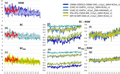
Figure 9.Average of standard deviations for the study domain, for the raw data(a), the BC(b)and the BC-NM(c)for the different models and the observations, on an annual basis. Differences between the raw and the bias-corrected standard deviations are shown in(d)and(e). Plots(f)and(g)correspond to the same data as(d)and(e), but normalized for their 1951–2005 mean.
overestimation. In contrast, with the use of NM the change in the trend is reduced in most of the European area.
The impact of NM on the standard deviation is also signif-icant. Figure 9 shows the evolution of the standard deviations of the adjusted daily data for each model, in the cases of raw data and the bias-corrected data using the BC and the BC-NM. The standard deviation is estimated for each grid point and calendar year, and is averaged across the study domain. The results show that the standard deviation of the adjusted data differs from the respective standard deviations of the raw data, in both adjustment approaches. This is an expected outcome, as raw model data standard deviations differ from the respective observed data standard deviation (Fig. 9d, e). However, the standard deviation differences between BC-NM and the raw data (Fig. 9f) are significantly more stable than the respective differences from BC (Fig. 9g), meaning that the signal of standard deviation is better preserved and does not inflate significantly with time in the former case. Additionally, the variation of the standard deviations time se-ries exhibits lower fluctuations.
5 Discussion
This study focuses on known issues of bias correction that have been well discussed in the literature. Whether the long-term signal of temperature should be preserved or not has
been discussed on a more theoretical level in Maraun (2016), while Haerter et al. (2011) mention that a credible bias cor-rection methodology should involve the consequences of greenhouse gas concentration changes. This is somehow con-sistent with the temperature trend preservation as the model sensitivity is retained in the corrected time series. As pointed in Fischer et al. (2012), models tend to underestimate the inter-annual variability due to deficiencies between land– atmosphere interactions, which urges for its correction. Nev-ertheless, the long-term statistics’ preservation may be neces-sitated in cases that temperature is used in biophysical impact modeling (Rubino et al., 2016), or may be preferred as a safer option than the unintentional alteration, especially in cases where the observational data record is not long enough.
Comparisons can also be performed with the methodology of Li et al. (2010), who use the differences in the raw data between the reference period and the projection period. In the present study the differences are defined between the ref-erence period and each year of correction separately. This can be considered as an evolution of the technique that over-comes the subjectivity of the future period selection. Addi-tionally, the quantile mapping correction ensures the skillful correction in the higher and lower quantiles, relative to sim-pler additive approaches such as that of Hempel et al. (2013), which, while preserving the trend and year-to-year variabil-ity, marginally improves the tails of the temperature distribu-tion (Sippel et al., 2016). Regarding the simpler BC-TREND version that was used for the central England example, it was found that it tends to preserve the long-term statistics as also noted by Cannon et al. (2015), but the 5-year average that was used for the trend preservation still cannot encompass the changes in each year’s CDF, as the NM can.
Beyond these advancements, a critical drawback of the presented methodology is that it uses a large number of pa-rameters to approximate the transfer functions in the two stages of the correction. The methodology can be described as of “varying complexity” as the number of the estimated parameters (number of segments) and the added value of the complexity is weighted by an information criterion. Nonethe-less, it is highly invasive, which means that in the case that high-noise observations were used, it would lead to trans-fer of that noise to the corrected data variability. This was marginally detected in the analysis of the standard devia-tions in Fig. 9, even if the effect of the BC-NM mitigated the effect compared to the BC. Another weakness stems from the residuals’ exclusion from the correction. In the theoret-ical case where the future projected temperature variability changes radically relative to the reference period, the correc-tion would result in larger remaining biases as it was shown earlier, which could impair the physical continuity of the time series. This limitation should be taken into consider-ation for the case that the BC-NM is used to correct other types of variables, without forbidding its use on them.
6 Conclusions
This study elaborates the issue of the distortion of the long-term statistics in quantile mapping statistical bias correction relative to the raw model data. An extra processing step is presented that can be applied along with quantile mapping statistical bias correction techniques. This step, namely NM, splits the original data into two parts – a normalized one that is bias adjusted using quantile mapping, and a residu-als part that is added to the former after the bias correction. The methodology is tested and validated from several points of view, leading to some key remarks about its added value. First, it is shown that the use of the NM module results in the long-term temperature trend preservation of the mean
tem-perature change, as well as of the trend in the higher and lower percentiles. Furthermore, the examination of the stan-dard deviation temporal evolution shows that it is better re-tained relative to the raw data, as the exclusion of the resid-uals from the correction minimizes the inflation of the vari-ance. Additionally, the inter-annual variability of the raw data is preserved relative to the compared simpler quantile map-ping methods, which is an important feature for climate im-pact studies that involve carbon cycle simulations (Rubino et al., 2016). Another noteworthy feature of the proposed method is that the normalization is performed on an annual basis; hence, the projection period results are not affected by the length of the projection period. Nevertheless, it has to be stressed that a range of issues – such as the disruption of the physical consistency of climate variables, the mass/energy balance and the omission of correction feedback mechanisms to other climate variables (Ehret et al., 2012) – were not ex-amined in this work, despite the existence of methods that preserve consistency between specific variables (Sippel et al., 2016). As an epilogue, bias correction cannot add further ac-curacy to the data but rather add usefulness to it, depending on the needs of each application. Nevertheless, it should not be underestimated that this added usefulness may obscure a deterioration of the climate change signal owing to the bias correction.
Data availability. All the underlying research data are freely ac-cessible. The RCM data were obtained from the Earth System Grid Federation (ESGF – https://esg-dn1.nsc.liu.se/search/cordex/, Ja-cob et al., 2014). The E-OBS data were obtained from the Euro-pean Climate Assessment & Dataset project website (http://www. ecad.eu, Haylock et al., 2008). The HadCET temperature data were obtained from the Met Office website (https://www.metoffice.gov. uk/hadobs/hadcet/, Parker et al., 1992).
The Supplement related to this article is available online at https://doi.org/10.5194/esd-8-889-2017-supplement.
Competing interests. The authors declare that they have no con-flict of interest.
We also thank the climate modeling groups (listed in Table 1 of this paper) for producing and making available their model output. Fi-nally, we acknowledge the E-OBS dataset from the ENSEMBLES EU-FP6 project (http://ensembles-eu.metoffice.com) and the data providers in the ECA&D project (http://www.ecad.eu).
Edited by: Axel Kleidon
Reviewed by: Stefan Hagemann and one anonymous referee
References
Bürger, G., Sobie, S. R., Cannon, A. J., Werner, A. T., and Mur-dock, T. Q.: Downscaling Extremes: An Intercomparison of Mul-tiple Methods for Future Climate, J. Climate, 26, 3429–3449, https://doi.org/10.1175/JCLI-D-12-00249.1, 2013.
Cannon, A. J., Sobie, S. R., and Murdock, T. Q.: Bias Correction of GCM Precipitation by Quantile Mapping: How Well Do Methods Preserve Changes in Quantiles and Extremes?, J. Climate, 28, 6938–6959, https://doi.org/10.1175/JCLI-D-14-00754.1, 2015. Christensen, J. H., Boberg, F., Christensen, O. B., and
Lucas-Picher, P.: On the need for bias correction of regional climate change projections of temperature and precipitation, Geophys. Res. Lett., 35, L20709, https://doi.org/10.1029/2008GL035694, 2008.
Daliakopoulos, I. N., Tsanis, I. K., Koutroulis, A. G., Kourgialas, N. N., Varouchakis, E. A., Karatzas, G. P., and Ritsema, C. J.: The Threat of Soil Salinity: a European scale review, Sci. Total Environ., 573, 727–739, 2016.
Ehret, U., Zehe, E., Wulfmeyer, V., Warrach-Sagi, K., and Liebert, J.: HESS Opinions “Should we apply bias correction to global and regional climate model data?”, Hydrol. Earth Syst. Sci., 16, 3391–3404, https://doi.org/10.5194/hess-16-3391-2012, 2012. Fischer, E. M., Rajczak, J., and Schär, C.: Changes in European
summer temperature variability revisited, Geophys. Res. Lett., 39, L19702, https://doi.org/10.1029/2012GL052730, 2012. Geisser, S.: Predictive inference, CRC press, New York, 1993. Grillakis, M. G., Koutroulis, A. G., and Tsanis, I. K.:
Cli-mate change impact on the hydrology of Spencer Creek wa-tershed in Southern Ontario, Canada. J. Hydrol., 409, 1–19, https://doi.org/10.1016/j.jhydrol.2011.06.018, 2011.
Grillakis, M. G., Koutroulis, A. G., and Tsanis, I. K.: Mul-tisegment statistical bias correction of daily GCM precip-itation output, J. Geophys. Res.-Atmos., 118, 3150–3162, https://doi.org/10.1002/jgrd.50323, 2013.
Grillakis, M. G., Koutroulis, A. G., Papadimitriou, L. V., Dali-akopoulos, I. N., and Tsanis, I. K.: Climate-Induced Shifts in Global Soil Temperature Regimes, Soil Sci., 181, 264–272, https://doi.org/10.1097/SS.0000000000000156, 2016.
Haerter, J. O., Hagemann, S., Moseley, C., and Piani, C.: Climate model bias correction and the role of timescales, Hydrol. Earth Syst. Sci., 15, 1065–1079, https://doi.org/10.5194/hess-15-1065-2011, 2011.
Hagemann, S., Chen, C., Clark, D. B., Folwell, S., Gosling, S. N., Haddeland, I., Hanasaki, N., Heinke, J., Ludwig, F., Voss, F., and Wiltshire, A. J.: Climate change impact on available water resources obtained using multiple global cli-mate and hydrology models, Earth Syst. Dynam., 4, 129–144, https://doi.org/10.5194/esd-4-129-2013, 2013.
Hansen, J. W., Challinor, A., Ines, A. V. M., Wheeler, T., and Mo-ron, V.: Translating climate forecasts into agricultural terms: ad-vances and challenges, Clim. Res., 33, 27–41, 2006.
Harding, R. J., Weedon, G. P., van Lanen, H. A. J., and Clark, D. B.: The future for global water assessment, J. Hydrol., 518, 186–193, https://doi.org/10.1016/j.jhydrol.2014.05.014, 2014.
Hasumi, H. and Emori, S.: K-1 Coupled GCM (MIROC) Descrip-tion K-1 model developers, Tokyo, 2004.
Hawkins, E., Sutton, R., Hawkins, E., and Sutton, R.: Connect-ing Climate Model Projections of Global Temperature Change with the Real World, B. Am. Meteorol. Soc., 97, 963–980, https://doi.org/10.1175/BAMS-D-14-00154.1, 2016.
Haylock, M. R., Hofstra, N., Klein Tank, A. M. G., Klok, E. J., Jones, P. D., and New, M.: A European daily high-resolution gridded data set of surface temperature and pre-cipitation for 1950–2006, J. Geophys. Res., 113, D20119, https://doi.org/10.1029/2008JD010201, 2008 (data available at: http://www.ecad.eu).
Hempel, S., Frieler, K., Warszawski, L., Schewe, J., and Piontek, F.: A trend-preserving bias correction – the ISI-MIP approach, Earth Syst. Dynam., 4, 219–236, https://doi.org/10.5194/esd-4-219-2013, 2013.
Hofstra, N., New, M., and McSweeney, C.: The influence of in-terpolation and station network density on the distributions and trends of climate variables in gridded daily data, Clim. Dynam., 35, 841–858, https://doi.org/10.1007/s00382-009-0698-1, 2010. Huybers, P. and Curry, W.: Links between annual, Milankovitch and continuum temperature variability, Nature, 441, 329–332, https://doi.org/10.1038/nature04745, 2006.
Ines, A. V. M. and Hansen, J. W.: Bias correction of daily GCM rainfall for crop simulation studies, Agric. For. Meteorol., 138, 44–53, https://doi.org/10.1016/j.agrformet.2006.03.009, 2006. Jacob, D., Petersen, J., Eggert, B., Alias, A., Christensen, O. B.,
Bouwer, L. M., Braun, A., Colette, A., Déqué, M., Georgievski, G., Georgopoulou, E., Gobiet, A., Menut, L., Nikulin, G., Haensler, A., Hempelmann, N., Jones, C., Keuler, K., Ko-vats, S., Kröner, N., Kotlarski, S., Kriegsmann, A., Martin, E., van Meijgaard, E., Moseley, C., Pfeifer, S., Preuschmann, S., Radermacher, C., Radtke, K., Rechid, D., Rounsevell, M., Samuelsson, P., Somot, S., Soussana, J.-F., Teichmann, C., Valentini, R., Vautard, R., Weber, B., and Yiou, P.: EURO-CORDEX: new high-resolution climate change projections for European impact research, Reg. Environ. Chang., 14, 563–578, https://doi.org/10.1007/s10113-013-0499-2, 2014 (data available at: https://esg-dn1.nsc.liu.se/search/cordex/).
Klemes, V.: Operational testing of hydrological simulation models, Hydrol. Sci. J., 31, 13–24, https://doi.org/10.1080/02626668609491024, 1986.
Knutti, R.: The end of model democracy?, Clim. Change, 102, 395– 404, https://doi.org/10.1007/s10584-010-9800-2, 2010. Kotlarski, S., Keuler, K., Christensen, O. B., Colette, A., Déqué,
M., Gobiet, A., Goergen, K., Jacob, D., Lüthi, D., van Meij-gaard, E., Nikulin, G., Schär, C., Teichmann, C., Vautard, R., Warrach-Sagi, K., and Wulfmeyer, V.: Regional climate model-ing on European scales: a joint standard evaluation of the EURO-CORDEX RCM ensemble, Geosci. Model Dev., 7, 1297–1333, https://doi.org/10.5194/gmd-7-1297-2014, 2014.
wa-ter availability at +2◦C and +3◦C for east Mediterranean island states: The case of Crete, J. Hydrol., 532, 16–28, https://doi.org/10.1016/j.jhydrol.2015.11.015, 2016.
Kyselý, J. and Plavcová, E.: A critical remark on the applicabil-ity of E-OBS European gridded temperature data set for validat-ing control climate simulations, J. Geophys. Res., 115, D23118, https://doi.org/10.1029/2010JD014123, 2010.
Li, H., Sheffield, J., and Wood, E. F.: Bias correction of monthly precipitation and temperature fields from Intergovern-mental Panel on Climate Change AR4 models using equidis-tant quantile matching, J. Geophys. Res., 115, D10101, https://doi.org/10.1029/2009JD012882, 2010.
Maraun, D.: Bias Correcting Climate Change Simulations – a Critical Review, Curr. Clim. Chang. Reports, 2, 211–220, https://doi.org/10.1007/s40641-016-0050-x, 2016.
Maraun, D., Wetterhall, F., Ireson, A. M., Chandler, R. E., Kendon, E. J., Widmann, M., Brienen, S., Rust, H. W., Sauter, T., The-meßl, M., Venema, V. K. C., Chun, K. P., Goodess, C. M., Jones, R. G., Onof, C., Vrac, M., and Thiele-Eich, I.: Precipita-tion downscaling under climate change: Recent developments to bridge the gap between dynamical models and the end user, Rev. Geophys., 48, RG3003, https://doi.org/10.1029/2009RG000314, 2010.
Maurer, E. P. and Pierce, D. W.: Bias correction can modify cli-mate model simulated precipitation changes without adverse ef-fect on the ensemble mean, Hydrol. Earth Syst. Sci., 18, 915– 925, https://doi.org/10.5194/hess-18-915-2014, 2014.
Nikulin, G., Bosshard, T., Yang, W., Barring, L., Wilcke, R., Vrac, M., Vautard, R., Noel, T., Gutierrez, J. M., Herrera, S., Fernan-dez, J., Haugen, J. E., Benestad, R., Landgren, O. A., Grillakis, M., Tsanis, I., Koutroulis, A., Dosio, A., Ferrone, A., and Swi-tanek, M.: Bias Correction Intercomparison Project (BCIP): an introduction and the first results, EGU General Assembly Con-ference Abstracts, p. 2250, 2015.
Olsson, T., Jakkila, J., Veijalainen, N., Backman, L., Kaurola, J., and Vehviläinen, B.: Impacts of climate change on temperature, precipitation and hydrology in Finland – studies using bias cor-rected Regional Climate Model data, Hydrol. Earth Syst. Sci., 19, 3217–3238, https://doi.org/10.5194/hess-19-3217-2015, 2015. Papadimitriou, L. V., Koutroulis, A. G., Grillakis, M. G., and Tsanis,
I. K.: The effect of GCM biases on global runoff simulations of a land surface model, Hydrol. Earth Syst. Sci., 21, 4379–4401, https://doi.org/10.5194/hess-21-4379-2017, 2017.
Papadimitriou, L. V., Koutroulis, A. G., Grillakis, M. G., and Tsanis, I. K.: High-end climate change impact on European runoff and low flows – exploring the effects of forcing biases, Hydrol. Earth Syst. Sci., 20, 1785–1808, https://doi.org/10.5194/hess-20-1785-2016, 2016.
Parker, D. and Horton, B.: Uncertainties in central England tem-perature 1878–2003 and some improvements to the maxi-mum and minimaxi-mum series, Int. J. Climatol., 25, 1173–1188, https://doi.org/10.1002/joc.1190, 2005.
Parker, D. E., Legg, T. P., and Folland, C. K.: A new daily cen-tral England temperature series, 1772–1991, Int. J. Climatol., 12, 317–342, https://doi.org/10.1002/joc.3370120402, 1992 (data available at: https://www.metoffice.gov.uk/hadobs/hadcet/). Pierce, D. W., Cayan, D. R., Maurer, E. P., Abatzoglou, J.
T., Hegewisch, K. C., Pierce, D. W., Cayan, D. R., Mau-rer, E. P., Abatzoglou, J. T., and Hegewisch, K. C.: Im-proved Bias Correction Techniques for Hydrological Simula-tions of Climate Change, J. Hydrometeorol., 16, 2421–2442, https://doi.org/10.1175/JHM-D-14-0236.1, 2015.
Prein, A. F., Gobiet, A., Truhetz, H., Keuler, K., Goergen, K., Te-ichmann, C., Fox Maule, C., van Meijgaard, E., Déqué, M., Nikulin, G., Vautard, R., Colette, A., Kjellström, E., and Jacob, D.: Precipitation in the EURO-CORDEX 0.11◦and 0.44◦ simu-lations: high resolution, high benefits?, Clim. Dynam., 46, 383– 412, https://doi.org/10.1007/s00382-015-2589-y, 2015. Rubino, M., Etheridge, D. M., Trudinger, C. M., Allison, C. E.,
Rayner, P. J., Enting, I., Mulvaney, R., Steele, L. P., Langen-felds, R. L., Sturges, W. T., Curran, M. A. J., and Smith, A. M.: Low atmospheric CO2levels during the Little Ice Age due
to cooling-induced terrestrial uptake, Nat. Geosci., 9, 691–694, https://doi.org/10.1038/ngeo2769, 2016.
Sharma, D., Das Gupta, A., and Babel, M. S.: Spatial disaggrega-tion of bias-corrected GCM precipitadisaggrega-tion for improved hydro-logic simulation: Ping River Basin, Thailand, Hydrol. Earth Syst. Sci., 11, 1373–1390, https://doi.org/10.5194/hess-11-1373-2007, 2007.
Sippel, S., Otto, F. E. L., Forkel, M., Allen, M. R., Guillod, B. P., Heimann, M., Reichstein, M., Seneviratne, S. I., Thonicke, K., and Mahecha, M. D.: A novel bias correction methodology for climate impact simulations, Earth Syst. Dynam., 7, 71–88, https://doi.org/10.5194/esd-7-71-2016, 2016.
Teutschbein, C. and Seibert, J.: Bias correction of regional climate model simulations for hydrological climate-change impact stud-ies: Review and evaluation of different methods, J. Hydrol., 456, 12–29, https://doi.org/10.1016/j.jhydrol.2012.05.052, 2012. Themeßl, M. J., Gobiet, A., and Heinrich, G.: Empirical-statistical