www.nonlin-processes-geophys.net/24/101/2017/ doi:10.5194/npg-24-101-2017
© Author(s) 2017. CC Attribution 3.0 License.
Conditional nonlinear optimal perturbations based on
the particle swarm optimization and their applications
to the predictability problems
Qin Zheng1, Zubin Yang1, Jianxin Sha2, and Jun Yan1
1Institute of Science, PLA University of Science and Technology, Nanjing, 211101, China 2Troop 94906, People’s Liberation Army, Suzhou, 215157, China
Correspondence to:Zubin Yang ([email protected])
Received: 25 September 2016 – Discussion started: 21 October 2016
Revised: 18 January 2017 – Accepted: 1 February 2017 – Published: 22 February 2017
Abstract.In predictability problem research, the conditional nonlinear optimal perturbation (CNOP) describes the initial perturbation that satisfies a certain constraint condition and causes the largest prediction error at the prediction time. The CNOP has been successfully applied in estimation of the lower bound of maximum predictable time (LBMPT). Gen-erally, CNOPs are calculated by a gradient descent algorithm based on the adjoint model, which is called ADJ-CNOP. This study, through the two-dimensional Ikeda model, investigates the impacts of the nonlinearity on ADJ-CNOP and the corre-sponding precision problems when using ADJ-CNOP to es-timate the LBMPT. Our conclusions are that (1) when the initial perturbation is large or the prediction time is long, the strong nonlinearity of the dynamical model in the prediction variable will lead to failure of the ADJ-CNOP method, and (2) when the objective function has multiple extreme val-ues, ADJ-CNOP has a large probability of producing local CNOPs, hence making a false estimation of the LBMPT. Fur-thermore, the particle swarm optimization (PSO) algorithm, one kind of intelligent algorithm, is introduced to solve this problem. The method using PSO to compute CNOP is called PSO-CNOP. The results of numerical experiments show that even with a large initial perturbation and long prediction time, or when the objective function has multiple extreme values, PSO-CNOP can always obtain the global CNOP. Since the PSO algorithm is a heuristic search algorithm based on the population, it can overcome the impact of nonlinearity and the disturbance from multiple extremes of the objective function. In addition, to check the estimation accuracy of the LBMPT presented by PSO-CNOP and ADJ-CNOP, we
par-tition the constraint domain of initial perturbations into suf-ficiently fine grid meshes and take the LBMPT obtained by the filtering method as a benchmark. The result shows that the estimation presented by PSO-CNOP is closer to the true value than the one by ADJ-CNOP with the forecast time in-creasing.
1 Introduction
Based on actual demands, Mu et al. (2002) separated the predictability problem into three sub-problems, i.e., the prob-lem of the LBMPT, the probprob-lem of the upper bound of maxi-mum prediction error, and the problem of the lower bound of maximum allowable initial error and parameter error. Duan and Luo (2010) formulated these three problems into three constrained nonlinear optimization problems. Meanwhile, they used the CNOP method to find the solutions of the three sub-problems.
Capturing CNOPs is a kind of constraint optimization problem, and optimization algorithms commonly used in solving CNOPs are based on the gradient descent method, including the spectral projected gradient 2 (SPG2; Brigin et al., 2000), sequential quadratic programming (SQP; Powell, 1982), and limited memory BFGS (L-BFGS; Liu and No-cedal, 1989). Among these algorithms, the gradient informa-tion is always provided by the backward integral of the corre-sponding adjoint model of the prediction model (Duan et al., 2004, 2008; Mu and Zhang, 2006; Mu et al., 2009; Jiang and Wang, 2010; Yu et al., 2012; Wang et al., 2012, 2013). But the optimal algorithms based on gradient information involve the forward integral of the tangent model and backward in-tegration of the adjoint model. It might cause the following two problems: (1) for the numerical prediction model with complex physical processes, the validity of the tangent linear approximation cannot be guaranteed when the forecast pe-riod is long; (2) for the actual prediction model, it is quite difficult and time consuming to develop the adjoint model. Recently, Zheng et al. (2012, 2014) attempted to apply ge-netic algorithms (GAs) to capture CNOPs of the dynami-cal model containing discontinuous “on–off” switches. They concluded that GAs, with proper genetic operator configu-ration, can overcome the non-smooth influences and obtain the global CNOP with high probability. Thus, in non-smooth cases, using GAs to solve predictability problems is more ef-fective than using the conventional optimization algorithm.
The particle swarm optimization (PSO) algorithm is an intelligent algorithm proposed by Kennedy and Eber-hart (1995) which imitated the process of bird foraging. In the PSO algorithm, each particle, as a vector in solution space, represents a potential solution of the optimal
prob-highly precise estimation of the lower bound of maximum predictable time.
The Ikeda model was originally proposed by Ikeda (1979) as a model describing light going across a nonlinear opti-cal resonator. The Ikeda model has strong nonlinearity, and the two-dimensional difference scheme is its most common form. Li et al. (2016) investigated the stability of solutions of the Ikeda model and tested the dependence of the solu-tions on the model parameter. In addition, they provided the solution description of various shapes corresponding to pa-rameter values of different regions. This paper takes the two-dimensional Ikeda model as the prediction model to reveal how the nonlinearity impacts the precision when estimat-ing the LBMPT based on the ADJ-CNOP method. A new method, PSO-CNOP, is presented to solve this problem.
This paper is organized as follows: Sect. 2 is devoted to de-scribing the three predictability sub-problems, the definition of CNOP and the two-dimensional Ikeda model. Section 3 provides the knowledge about the particle swarm optimiza-tion (PSO) algorithm. In Sect. 4, the performances of ADJ-CNOP and PSO-ADJ-CNOP are compared when solving ADJ-CNOPs through numerical experiments. The impacts on the estima-tion precision of the lower bound of maximum predictable time are also demonstrated in this section. The conclusion and discussion are presented in Sect. 5.
2 Related conceptions and the forecast model
Problem 1: the lower bound of maximum predictable time (LBMPT)
Assuming that there is an error in the initial condition (IC) of the forecast model, it will lead to a prediction error when integrating forward the model from the IC to predict the at-mospheric or oceanic states in the future.
Letu0be the IC,utT the true state at timeT, andMT the nonlinear propagator of the numerical forecast model from 0 to timeT; then, under the assumption of the perfect model, utT =MT(ut0), whereut0is the true state at the initial time.
With a given prediction precisionε >0, the maximum pre-dictable timeTεis defined as follows:
Tε=max{τ| ||MT(u0)−utT||2≤ε,0≤T ≤τ}. (1) Since the true valueutT cannot be obtained exactly, it is im-possible to getTεby solving the nonlinear optimization prob-lem (1). Inspired by the fact that the ICu0is often provided by an analysis field, and the associated analysis error can generally be controlled in a specified range, Mu et al. (2002) reduced the maximum predictable time problem to the fol-lowing LBMPT problem.
If we have an estimation of the uncertainty in the IC as follows,
u0−ut0
≤σ, (2)
then the LBMPTTlis defined as Tl= min
||δu0||≤σ
{Tu0,δu0|Tu0,δu0=maxτ,
||Mt(u0+δu0)−Mt(u0)|| ≤ε,0≤t≤τ}, (3) whereσ >0 denotes the accuracy of the IC in terms of the norm|| · ||, andδu0is an initial perturbation superposed on the IC. According to Eq. (2), the true initial state is within the constraint region; we have
Tl≤Tε.
Problem 2: the upper bound of maximum prediction error
When a forecast is produced from an incorrect initial ICu0, the prediction error at the prediction timeT is
E= ||MT(u0)−utT||. (4)
Similarly to problem 1, since the true valueutT cannot be ob-tained precisely, Mu et al. (2002) instead introduced the up-per bound of the maximum prediction error within the given initial error limitation as follows:
Eu= max ||δu0||≤σ
||MT(u0+δu0)−MT(u0)||. (5) Note that ut0 satisfies Eq. (2) and utT =MT(ut0)under the assumption of perfect model; we have
E≤Eu.
Problem 3: the lower bound of maximum allowable initial error
Given the prediction timeT >0 and prediction precisionε > 0, the maximum allowable initial error is
σmax=max{σ| ||MT(u0+δu0)−utT|| ≤ε,||δu0|| ≤σ}. (6) Similar to problems 1 and 2, the above problem was reduced by Mu et al. (2002) to the following lower bound of maxi-mum allowable initial error:
σmax=max{σ| ||MT(u0+δu0)−MT(u0)|| ≤ε,||δu0|| ≤σ}. (7)
2.2 Conditional nonlinear optimal perturbation (CNOP)
In consideration of the nonlinearity impacts, Mu et al. (2003) introduced CNOPs into the study of predictability problems. Suppose the atmospheric or oceanic motions can be de-scribed by the following dynamic system:
( ∂U
∂t +F(U, t )=0, U|t=0=U0,
(8)
whereU(x, t )=(U1(x, t ), U2(x, t ),· · ·, Un(x, t ))T is the ba-sic state, which is ann-dimensional vector; the superscript T represents the transpose,U0 is the initial basic state, and x=(x1, x2,· · ·, xm)T ∈⊂Rm and t are the spatial and temporal variables, respectively;t=0 is the initial time; and Fis a nonlinear partial differential operator.
Suppose Mτ is the nonlinear transmission propagator from the initial timet=0 to the forecast time t=τ; thus, the state of model (8) at timeτ is
U(x, τ )=Mτ(U0) . (9)
Ifu0stands for the initial perturbation of the basic stateU(t ) anduI(τ )is the development ofu0at timeτ, that is, uI(τ )=Mτ(U0+u0)−Mτ(U0), (10) then the initial perturbationu∗
0is called the conditional non-linear optimal perturbation (CNOP) if and only ifu∗0 is the solution of the following optimization problem:
J u∗0= max
u0∈Bσ
||Mτ(U0+u0)−Mτ(U0)||, (11)
where Bσ = {u0
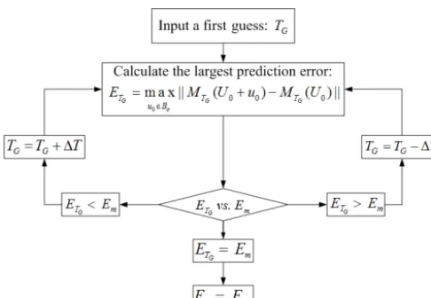
Figure 1.Flow chart of solving the LBMPT.
2.3 Estimation of the LBMPT
Duan and Luo (2010) designed a numerical method to cal-culate the LBMPT in their research of predictability (Fig. 1). It should be noted that CNOPs stand for the initial uncer-tainty in the given constrained domain which leads to the largest prediction error. Therefore, the maximum prediction error can be estimated by solving CNOPs.
In detail, for a given first guess valueTGof the prediction time, one can use a constraint nonlinear optimization algo-rithm to capture the CNOP so as to estimate the maximum prediction errorETG at timeTGcaused by the initial error in a constraint domainBσ.
IfETG > Em (Emstands for the allowable prediction er-ror), we try to reduce the integral time stepTG=TG−1T, where1T is a certain constant, and calculate the maximum prediction error at the reduced time. IfETG < Em, we will increase the integral time stepTG=TG+1T and calculate the maximum prediction error at the newTG.
If TG satisfies the conditions ETG+1T > Em and ETG−1T ≤Em, then TG is considered the lower bound of maximum predictable time which satisfies the prediction pre-cisionEm under the given initial error. The operation flow chart is shown as Fig. 1.
2.4 The two-dimensional Ikeda model
The following two-dimensional Ikeda model is adopted as the prediction model:
x1(t+1)=1+µ (x1(t )cosθt−x2(t )sinθt) x2(t+1)=µ (x1(t )sinθt+x2(t )cosθt) ,
(12)
θt=a−
b
1+x1(t )2+x2(t )2
, (13)
where 0≤µ≤1,a=0.4 andb=6.
From the expression of the model we find that the trigono-metric functions appear in Eq. (12), and Eq. (13) is a
frac-Figure 2.The distribution of solutions at the last 5000 steps when µ=0.83.
tion whose denominator includes two quadratic components. Thus, the two-dimensional Ikeda model has fairly strong nonlinearity (Li and Zheng, 2016). The solutions of the model present different behaviors with the change in the model parameter µ. When the parameter varies from 0 to 1, the numerical solutions change from a point attractor to periodic solutions, then to chaos, and end up with a limit cy-cle (Li and Zheng, 2016). The predictability problems are always launching under chaos. According to the conclusions given by Li and Zheng (2016), the model solution appeared chaotic whenµ∈ [0.700,0.902]. Figure 2 shows the numer-ical solution of the last 5000 steps in 10 000 integral steps, while the initial value is set to(x0, y0)=(0.25,−0.325)and the model parameter isµ=0.83.
The basic PSO algorithm consists of three processes, namely, generating particles’ positions and velocities, assess-ing particles, and updatassess-ing particles’ positions and velocities. The mathematical description of the classic PSO al-gorithm is as follows: in an n-dimensional search space, each particle of PSO represents a potential solution of the optimization problem. We denote M
the swarm size, Xi(k)=(xi1(k), xi2(k),· · ·, xi n(k)) and Vi(k)=(vi1(k), vi2(k),· · ·, vi n(k))the position and the ve-locity of the ith particle at the kth generation, respec-tively,Pi(k)=(pi1(k), pi2(k),· · ·, pi n(k))the personal his-torical best position of the ith particle found so far, and Pg(k)= pg1(k), pg2(k),· · ·, pg n(k)
the best position that the whole swarm attained so far; then the particlei’s veloc-ity and position in the nextk+1 generation can be updated according to the following formula:
vid(k+1)=w vid(k)+c1r1(pid(k)−xid(k))
+c2r2 pgd(k)−xid(k)
, (14)
xid(k+1)=xid(k)+vid(k+1), (15) where i=1,2,· · ·, M, d=1,2,· · ·, n, c1 and c2 are the acceleration coefficients, which make particles having the ability to self-summarize and learn from excellent particles among the group to approach their own and group historical optimal points. r1 andr2are two random numbers that are subject to uniform distribution on the interval[0,1].ωis the inertia weight. It can be set as a fixed constant or a linear reduction function with the increase in the evolutional gen-erations. The flow chart of the PSO algorithm is shown as Fig. 3.
When using a PSO to search CNOPs for the estimation of the LBMPT, the prediction error at the specified forecast time is the associated objective functionJ. The initial perturbation δu, which is a two-dimensional vector in the search space in our situation, is the optimization variable.
4 Numerical experiments and their results analyses 4.1 The numerical experiments solving CNOPs by
different optimization algorithms
In order to compare the performances of the ADJ-CNOP and PSO-CNOP in solving CNOPs, the CNOPs yielded by the filtering method are taken as the benchmark after fine-dividing the constraint domain of initial perturbations. The filtering method is implemented as follows. The correspond-ing circumscribed square of a constraint region of the CNOP is considered; four square meshes of a certain size are used to discretize the circumscribed square. For any mesh point outside the region, it is connected with the center of the re-gion; the intersection point of this line with the boundary of the region is obtained. Integrating the Ikeda model from the initial basic state superimposed each of these intersection
Figure 3.The flow chart of the PSO algorithm.
points and, for the mesh points inside the region, the predic-tion error caused by each initial error can be obtained. The CNOP refers to the mesh point which leads to the largest prediction error (Duan and Luo, 2010). Since the accuracy of the CNOP generated by the filtering method depends on the division size of the constraint region exclusively, the circum-scribed squares of the constraint ball of CNOPs are separated into 1001×1001 small quadrate patches with very small side length 1.6402×10⁻⁵ in numerical experiments. For a de-tailed description of the operation of the filtering method, one can refer to Duan and Luo (2010) and Zheng et al. (2012).
In the numerical experiments, the initial basic state of the two-dimensional Ikeda model is (x0, y0)=(0.25,−0.325), and the model parameter isµ=0.83. The population size of the PSO isM=60, the maximum evolutional generation is set to 200, inertia weight isω=0.729 and the accelerating factors areC1=2.05 andC2=2.05. The norms measuring IC errors and prediction errors are both theL2norm, and the radiusσ of the constraint ballBσ is 8.201×10⁻³.
The particle swarm initialization scheme in PSO-CNOP is as follows:
Xi =(xi,1(0), xi,2(0))are random vectors obeying a uniform distribution onBσ.
Vi(0)= vi,1(0), vi,2(0)=Xi(0), i=1,2,· · ·, M. The first guess of the perturbation δu=(x0, y0) for ADJ-CNOP is randomly picked fromBσ. The constrained opti-mization algorithm used in ADJ-CNOP is the SPG2.
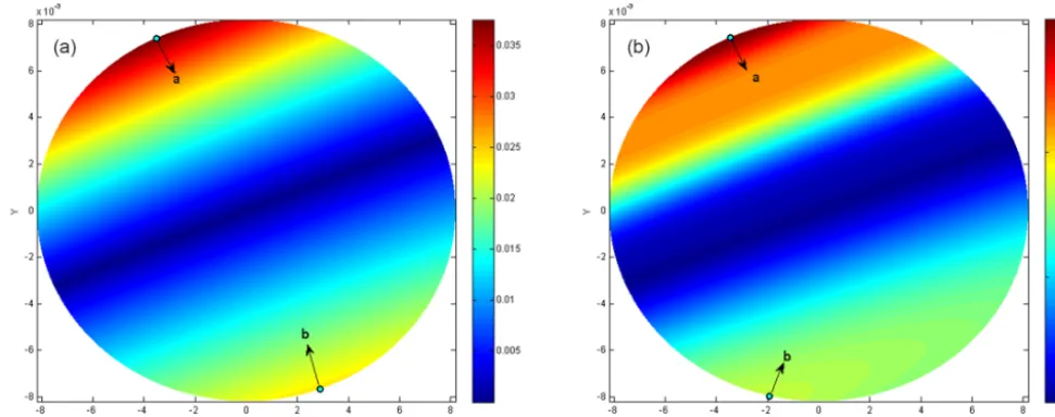
Figure 4.The distributions of OFVs at the prediction times 61t (left) and 131t (right), in which dots a and b are the global and local maximum points.
Table 1.Statistical analysis of CNOPs produced by different methods at 61t.
Method OFV CNOP Proportion
Filtering 3.7533×10⁻² (−3.5066×10⁻³, 7.4131×10⁻³)
ADJ-CNOP 3.7533×10⁻² (−3.5068×10⁻³, 7.4130×10⁻³) 47.5 % 2.3973×10⁻² (2.9072×10⁻³,−7.6683×10⁻³) 52.5 % PSO-CNOP 3.7533×10⁻² (−3.5068×10⁻³, 7.4130×10⁻³) 100 %
The numerical experiment results show that when the inte-gration time of the prediction model is short, the correspond-ing objective function (Eq. 11) presents good behavior with the change in the initial perturbation. It has only two extreme values in the constraint ball of the initial perturbation. One is the global maximum, and the extreme point corresponds to the global CNOP. The other is the local maximum, and the extreme point is a local CNOP. Figure 4 shows the distribu-tion of objective funcdistribu-tion values (OFVs) when the predicdistribu-tion times are on 6th unit time steps, i.e., 61t (left) and 131t (right), respectively, in which the global maximum point is located at point a and point b is the position of the local max-imum.
Tables 1 and 2 demonstrate the statistical analysis results of the CNOPs produced by ADJ-CNOP and PSO-CNOP when capturing CNOPs 40 times at the forecast times 61t and 131t, and the related results generated by the filtering method. Through the FCM method, we find that CNOPs ob-tained by the ADJ-CNOP method are divided into two cate-gories: one is related to the global CNOP that accounted for 47.5 % (70 %) for the forecast time 61t (131t )of the total; the other is the local CNOP that makes up 52.5 % (30 %) of the total. However, 40 CNOPs captured by PSO-CNOP are completely the same, and they are coincident with the CNOP yielded by the filtering method.
From Tables 1 and 2, we can see that although the pre-diction time is short, the ADJ-CNOP method still has a large probability of capturing local CNOPs, while PSO-CNOP can always catch the global CNOP. Actually, we can draw the same conclusion with the prediction time being increased to 131t.
When the forecast time increases to 141t, the 40 CNOPs yielded by ADJ-CNOP and PSO-CNOP are demonstrated in the following Fig. 5.
Figure 6 indicates all CNOPs generated by the filtering method with fine division of the constraint domain of ini-tial perturbations (the circumscribed squares of the constraint ball of CNOPs are separated into 1001×1001 small quadrate patches with very small side length 1.6402×10⁻⁵).
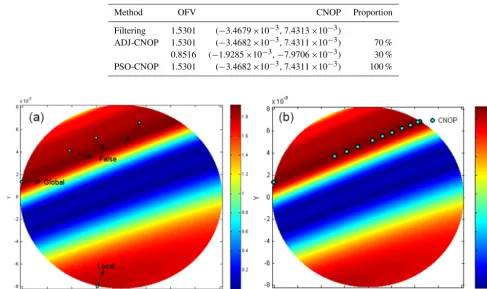
Table 2.Same as Table 1, except at 131t.
Method OFV CNOP Proportion
Filtering 1.5301 (−3.4679×10⁻³, 7.4313×10⁻³)
ADJ-CNOP 1.5301 (−3.4682×10⁻³, 7.4311×10⁻³) 70 % 0.8516 (−1.9285×10⁻³,−7.9706×10⁻³) 30 % PSO-CNOP 1.5301 (−3.4682×10⁻³, 7.4311×10⁻³) 100 %
Figure 5. The distributions of OFVs at the prediction time 141t, where the dots in the left (right) panel are the CNOPs produced by ADJ-CNOP (PSO-CNOP).
Figure 6.The distributions of OFVs at the prediction time 141t, where dots are the CNOPs produced by the filtering method.
Additionally, comparing the right panel of Fig. 5 with Fig. 6, it is easy to know that although many CNOPs are pro-duced by PSO-CNOP in 40 repeated numerical experiments,
all of the CNOP points are located on the same line as the one presented by the filtering method. Therefore, the CNOPs yielded by PSO-CNOP are all global.
When we keep extending the prediction time, the behavior of the objective function will get much worse, and more ex-treme points will appear. In order to verify the performance of the PSO-CONP method in solving CNOPs in the strong nonlinear case, the mean value and variance of the OFVs of the 40 CNOPs at different forecast times are calculated and compared with the maximal OFV (MOFV) obtained by the filtering method.
According to Table 3, the OFVs of 40 CNOPs calculated by the PSO-CNOP method at each forecast time are almost consistent with the maximum of the objective function got-ten by the filtering method at the same forecast time. There-fore, PSO-CNOP is still capable of solving global CNOPs of the two-dimensional Ikeda model for long forecast times. Figure 7 demonstrates the distributions of OFVs at the pre-diction times 151t, 181t and 221t, as well as the locations of all CNOPs generated by PSO-CNOP.
Figure 7.The distribution of OFVs at the prediction times 151t(the left of the upper panel), 181t(the right of the upper panel) and 221t (the lower panel), where dots denote CNOPs captured by PSO-CNOP.
Table 3.The precision analysis of the CNOPs produced by PSO-CNOP at different forecast times.
Prediction MOFV of the CFV of PSO-CNOP
time filtering method Mean value Variance
151t 1.6106 1.6106 3.3142×10⁻¹⁶ 161t 1.3052 1.3052 8.6189×10⁻¹⁴ 171t 1.6521 1.6521 2.0092×10⁻¹⁶ 181t 1.7807 1.7807 7.6313×10⁻¹⁷ 191t 1.5401 1.5401 1.7300×10⁻¹⁶ 201t 1.3482 1.3482 8.8314×10⁻¹⁰ 211t 1.6980 1.6980 3.3546×10⁻¹⁰ 221t 1.6602 1.6593 4.6798×10−07
distributions of OFVs at the prediction time 221t, it cannot be confirmed directly from the lower panel of Fig. 7 whether or not the CNOPs are global. Therefore, we select one CNOP randomly from each cluster of the 40 CNOPs and zoom into the graph nearby the CNOP point to look at the OFV
distri-bution. Figure 8 gives one of the results, from which we can see that the CNOP is still located in the maximal OFV area.
With further increasing of the prediction time, the strong nonlinearity deteriorates the behavior of the objective func-tion seriously. In this situafunc-tion, a predictability study based on the CNOP method becomes no longer meaningful because the CNOPs are too dispersive.
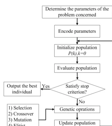
4.2 Comparison between PSO-CNOP and GA-CNOP In the following, the GA is adopted to capture CNOPs of the two-dimensional Ikeda model, and the results are compared with the ones obtained by the PSO-CNOP. The method using the GA to compute CNOP is called GA-CNOP. The relevant operational flow chart of the GA is shown in Fig. 9.
The configuration of the genetic operators and the relevant parameter are the same as in Zheng et al. (2014). A more detailed description of the GA and numerical experiment scheme of GA-CNOP can be found in Zheng et al. (2014).
Figure 8.Local distribution of the OFV at the prediction time 221t nearby the CNOP point.
Figure 9.The flow chart of the GA.
results are statistically analyzed and presented in Tables 4 and 5.
It can clearly be seen from Tables 4 and 5 that the op-timal population size of PSO-CNOP is about 15, but the optimal population size of GA-CNOP is about 40. Further-more, the computational times and CFV calculated, respec-tively, by PSO-CNOP with a population size of 15 and GA-CNOP with a population size of 40, are compared with that of ADJ-CNOP. Table 6 illustrates the mean CFV and the aver-age computation time obtained by different methods in their 40 numerical experiments.
Table 4.Mean CFV of 40 CNOPs produced by PSO-CNOP for every given population size.
Population size
Prediction 5 10 15 30 45 60
time
131t 1.5301 1.5301 1.5301 1.5301 1.5301 1.5301 191t 1.5209 1.5396 1.5401 1.5401 1.5401 1.5401
Table 5.Same as Table 4, except that 40 CNOPs are produced by GA-CNOP.
Population size
Prediction 16 26 36 40 50 60
time
131t 1.5299 1.5300 1.5300 1.5300 1.5300 1.5300 191t 1.5019 1.5295 1.5357 1.5400 1.5400 1.5400
From the numerical results we can see that the CFV of GA-CNOP is almost the same as PSO-CNOP; the GA is an effective optimal algorithm to obtain the optimal solution. However, the GA is more time consuming than PSO. At the same time, the computational time of PSO-CNOP and GA-CNOP is much greater than ADJ-GA-CNOP, which is also the difference between stochastic searching algorithms and de-terministic searching algorithms. Fortunately, in intelligent optimization algorithms, the parallel computation can be eas-ily realized. The operators of different individuals in one gen-eration are independent, and can be done in different CPUs, which thereby can take full advantage of fast developed par-allel computation technology (Fang et al., 2009).
4.3 Estimation of the LBMPT
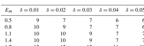
The CNOP method can be adopted to do a similar study on other two predictability sub-problems. Here we only focus on the estimation of the LBMPT to discuss the influence of nonlinearity. To demonstrate the effectiveness of PSO-CNOP in solving this problem, the filtering method, ADJ-CNOP and PSO-CNOP are used in the numerical experiments, re-spectively. In order to compare the estimation accuracy of the LBMPT generated by ADJ-CNOP and PSO-CNOP, the LBMPT computed by the filtering method with a fine divi-sion is taken as the benchmark. Different allowable predic-tion errors Em, 0.5, 0.8, 1.1, 1.4, and 1.7, and a different constrained radiusδof initial perturbations, 0.01, 0.02, 0.03, 0.04, and 0.05, are employed to verify the performance of the ADJ-CNOP and PSO-CNOP methods. The lattice spacing of the filtering method is 0.001. Tables 7, 8 and 9 illustrate the LBMPTs computed by the filtering method, PSO-CNOP and ADJ-CNOP, respectively.
0.5 9 7 7 6 6
0.8 10 9 7 7 6
1.1 10 10 9 7 7
1.4 10 10 9 7 7
1.7 12 12 12 11 10
Table 8.The LBMPT estimated by the PSO-CNOP method.
Em δ=0.01 δ=0.02 δ=0.03 δ=0.04 δ=0.05
0.5 9 7 7 6 6
0.8 10 9 7 7 6
1.1 10 10 9 7 7
1.4 10 10 9 7 7
1.7 12 12 12 11 10
worth mentioning that with the prediction time extending, al-though the objective functions have multiple extreme values and PSO-CNOP would produce different CNOPs in differ-ent numerical experimdiffer-ents, each one of these CNOPs can be used to estimate the maximum prediction error, and the final LBMPTs obtained are the same since they are all global.
The bold numbers in Table 9 are the LBMPTs that are dif-ferent from the ones computed by the filtering method. The LBMPTs yielded by the ADJ-CNOP method are generally larger. The reason is that the CNOP given by the ADJ-CNOP method is often local, even false. Therefore the estimation of the maximum prediction error based on the CNOP is usually questionable and untrusted.
To investigate the probability that the ADJ-CNOP method generates incorrect LBMPTs, we operate the numerical ex-periment shown in Table 9 40 times with various first guesses of the initial perturbations. The statistical analysis results are given in Table 10.
From Table 10, we can see that the ratio of incorrect LBMPTs based on ADJ-CNOP is high. The highest one even reaches 95 % whenδ=0.02 andEm=1.7. This problem is serious for real weather forecasts since it can mislead fore-casts with a large probability.
0.5 9 7 7 7 7
0.8 10 9 8 7 6
1.1 10 11 9 9 8
1.4 10 10 10 9 9
1.7 12 13 12 11 10
Table 10.Incorrect ratio in all 40 LBMPTs yielded by ADJ-CNOP.
Em δ=0.01 δ=0.02 δ=0.03 δ=0.04 δ=0.05
0.5 15 % 40 % 32.5 % 52.5 % 45 % 0.8 22.5 % 55 % 35 % 42.5 % 50 % 1.1 7.5 % 42.5 % 35 % 42.5 % 57.5 % 1.4 25 % 32.5 % 35 % 52.5 % 50 % 1.7 12.5 % 95 % 30 % 60 % 60 %
5 Conclusion and discussion
Since the two-dimensional Ikeda model has strong nonlin-earity, when we utilize the ADJ-CNOP method to capture CNOPs, not only global or local CNOPs, but even false CNOPs, are obtained. The reason for this is that in the case of strong nonlinearity, the gradient provided by the adjoint model is incorrect. When the traditional optimization algo-rithm uses a wrong descent direction to search for extreme values of the objective function, false CNOPs are presented. PSO is a heuristic search algorithm based on population. It can overcome the nonlinear influences and produce global CNOPs with high probability. In addition, the operation of the PSO algorithm is simple. This study applies the PSO al-gorithm to capture the CNOP of the two-dimensional Ikeda model. Numerical experiment results with different forecast times demonstrate that although the objective function has awful behavior and multiple extreme values, PSO-CNOP can still capture global CNOPs.
estimation of the LBMPT presented by PSO-CNOP is pre-cise. It is consistent with the one yielded by the filtering method with fine division.
As we know, our numerical experiments focus on two-dimensional prediction models only. When considering high-dimensional and more complex models, whether or not the classic PSO algorithm used in this study can overcome the influence of high dimensions and the computation time meet the real requirement is still unknown. The problems of the curse of dimensionality and multimodal function are a big challenge for almost all intelligent optimization algorithms, also PSO. Whether it can be effective in higher-dimensional and more complicated models deserves further research. In short, the PSO-CNOP approach is an alternative method to study predictability problems in the case of strong nonlinear-ity.
Competing interests. The authors declare that they have no conflict of interest.
Acknowledgements. This work was supported by the National Natural Science Foundation of China (grant nos. 41430426 and 41331174).
Edited by: J. Duan
Reviewed by: two anonymous referees
References
Banks, A., Vincent, J., and Anyakoha, C.: A review of particle swarm optimization. Part I: background and development, Nat. Comput., 6, 467–484, doi:10.1007/s11047-007-9049-5, 2007. Banks, A., Vincent, J., and Anyakoha, C.: A review of particle
swarm optimization. Part II: hybridisation, combinatorial, mul-ticriteria and constrained optimization, and indicative applica-tions, Nat. Comput., 7, 109–124, doi:10.1007/s11047-007-9050-z, 2008.
Birgin, E. G., Martinez, J. M., and Raydan, M.: Nonmonotone spec-tral projected gradient methods on convex sets, SIAM J. Opti-miz., 10, 1196–1211, 2000.
Borges, M. D and Hartmann, D. L.: Barotropic Instability and Op-timal Perturbations of Observed Nonzonal Flows, J. Atmos. Sci., 49, 335–353, 1992.
Buizza, R. and Palmer, T. N.: The Singular-Vector Structure of the Atmospheric Global Circulation, J. Atmos. Sci., 52, 1434–1456, 1995.
Clerc, M. and Kennedy, J.: The particle swarm: Explosion, stability, and convergence in a multi-dimensional complex space, IEEE T. Evolut. Comput., 6, 58–73, 2002.
Duan, W. S. and Luo, H. Y.: A New Strategy for Solving a class of Constrained Nonlinear Optimization Problems Related to Weather and Climate Predictability, Adv. Atmos. Sci., 27, 741– 749, doi:10.1007/s00376-009-9141-0, 2010.
Duan, W. S., Mu, M., and Wang, B.: Conditional nonlinear optimal perturbation as the optimal precursors for ENSO events, J. Geo-phys. Res., 109, D23105, doi:10.1029/2004JD004756, 2004. Duan, W. S., Xue, F., and Mu, M.: Investigating a nonlinear
charac-teristic of El Niño events by conditional nonlinear optimal per-turbation, Atmos. Res., 94, 10–18, 2008.
Eberhart, R. C. and Shi, Y.: Particle swarm optimization: devel-opments, applications and resources, Congress on Evolutionary Computation, 37–30 May 2001, Korea, 1, 81–86, 2001. Fang, C. L. and Zheng, Q.: The effectiveness of a genetic algorithm
in capturing conditional nonlinear perturbation with parameteri-zation “on-off” switches included by a model, J. Trop. Meteorol., 13, 13–19, 2009.
Farrell, B. F.: Small error dynamics and the predictability of atmo-spheric flows, J. Atmos. Sci., 47, 2409–2416, 1990.
Hassan R., Cohanim B., De Weck O, and Venter G.: A Compari-son of Particle Swarm Optimization and the Genetic Algorithm [C], Proceedings of the 1st AIAA multidisciplinary design opti-mization specialist conference, 18–21 April 2005, Austin, Texas, 1897, 2005.
Ikeda, K.: Multiple-valued stationary state and its instability of the transmitted light by a ring cavity system, J. Opt. Commum., 30, 257–261, 1979.
Jiang, Z. N. and Wang, D. H.: A study on precursors to blocking anomalies in climatological flows by using conditional nonlinear optimal perturbations, Q. J. Roy. Meteor. Soc., 136, 1170–1180, 2010.
Kalnay, E.: Atmospheric modeling, data assimilation and pre-dictability [M], Cambridge university press, UK, 2003. Kennedy, J. and Eberhart, R. C.: Particle swarm optimization, in:
Proceedings of the 1995 IEEE international conference on neural networks, Perth, Australia, Piscataway, NJ: IEEE Service Center, 27 November–1 December 1995, 1942–1948, 1995.
Lacarra, J. F. and Talagrand, O.: Short-range evolution of small per-turbations in a baratropic model, Tellus, 40, 81–95, 1988. Li, Q., Zheng, Q., and Zhou, S. Z.: Study on the dependence of the
two-dimensional Ikeda model on the parameter, Atmos. Ocean. Sci. Lett., 9, 1–6, doi:10.1080/16742834.2015.1128694, 2016. Liu, D. C. and Nocedal, J.: On the limited memory BFGS method
for large scale optimization, Math. Program., 45, 503–528, 1989. Lorenz, E. N.: Climate predictability. The Physical Basis of Climate Modeling, WMO GARP Publ. Ser. No. 16, WMO, Sweden, 132– 136, 1975.
Mu, M. and Duan, W. S.: A new approach to studying ENSO pre-dictability: Conditional nonlinear optimal perturbation, Chinese Sci. Bull., 48, 1045–1047, 2003.
Mu, M. and Zhang, Z. Y.: Conditional nonlinear optimal pertur-bation of a two-dimensional quasigeostrophic model, J. Atmos. Sci., 63, 1587–1604, 2006.
Mu, M., Duan, W. S., and Wang, J. C.: The predictability problems in numerical weather and climate prediction, Adv. Atmos. Sci., 19, 191–204, 2002.
Mu, M., Wang, H. L., and Zhou, F. F.: A preliminary application of conditional nonlinear optimal perturbation to adaptive observa-tion, J. Atmos. Sci., 31, 1102–1112, 2007.