* Corresponding author
E-mail: [email protected] (A. S. Hameed) 2020 Growing Science Ltd.
doi: 10.5267/j.ijiec.2019.6.005
International Journal of Industrial Engineering Computations 11 (2020) 51–72
Contents lists available at GrowingScience
International Journal of Industrial Engineering Computations
homepage: www.GrowingScience.com/ijiec
A new hybrid approach based on discrete differential evolution algorithm to enhancement solutions of quadratic assignment problem
Asaad Shakir Hameeda*, Burhanuddin Mohd Aboobaidera, Modhi Lafta Mutara and Ngo Hea
Choona
Hang Tuah Jaya, 76100, Durian ,
Communication Technology, Universiti Teknikal Malaysia Melaka Faculty of Information and
a
Tunggal, Melaka, Malaysia
C H R O N I C L E A B S T R A C T
Article history: Received April 1 2019 Received in Revised Format June 19 2019
Accepted June 19 2019 Available online June 19 2019
The Combinatorial Optimization Problem (COPs) is one of the branches of applied mathematics and computer sciences, which is accompanied by many problems such as Facility Layout Problem (FLP), Vehicle Routing Problem (VRP), etc. Even though the use of several mathematical formulations is employed for FLP, Quadratic Assignment Problem (QAP) is one of the most commonly used. One of the major problems of Combinatorial NP-hard Optimization Problem is QAP mathematical model. Consequently, many approaches have been introduced to solve this problem, and these approaches are classified as Approximate and Exact methods. With QAP, each facility is allocated to just one location, thereby reducing cost in terms of aggregate distances weighted by flow values. The primary aim of this study is to propose a hybrid approach which combines Discrete Differential Evolution (DDE) algorithm and Tabu Search (TS) algorithm to enhance solutions of QAP model, to reduce the distances between the locations by finding the best distribution of N facilities to N locations, and to implement hybrid approach based on discrete differential evolution (HDDETS) on many instances of QAP from the benchmark. The performance of the proposed approach has been tested on several sets of instances from the data set of QAP and the results obtained have shown the effective performance of the proposed algorithm in improving several solutions of QAP in reasonable time. Afterwards, the proposed approach is compared with other recent methods in the literature review. Based on the computation results, the proposed hybrid approach outperforms the other methods.
© 2020 by the authors; licensee Growing Science, Canada Keywords:
Combinatorial optimization Problems
Facility Layout Problem Quadratic Assignment Problem Discrete Differential Evolution Algorithm
Tabu Search Algorithm
1. Introduction
layout problems, but most of them have only focused on studying facility layout problems in manufacturing facilities, with just a few of them analyzing this problem within hospital domain. The modelling of FLP was first carried out as a quadratic assignment problem (QAP) by (Koopmans & Beckmann, 1957). According to Samanta et al. (2018), these COPs emerge from real-life situations. The use of discrete formulations is employed in layout problems which involve determining possible positions of facilities prior to their optimization. QAP is commonly used for this kind of problem. The QAP is regarded as a problem of NP-Hard combinatorial optimization (Şahinkoç & Bilge, 2018), which serves as a model for many real-life applications such as hospital layout, backboard wiring, campus layout, scheduling and designing of keyboard typewriter, etc. ever since the QAP was formulated, the attention of researchers has been drawn to it because of its importance in theory and practice, and most importantly because of how complex it is (Duman et al., 2012; Benlic & Hao, 2013; Kaviani et al., 2014;
Abdel-Basset et al., 2018a, Cela et al., 2018). The FLP has been introduced as a QAP in order to identify
the ideal allocation of N facilities to N locations, where there must be equality between the number of
locations and number of facilities. Researchers around the world have accepted the complexity associated with finding a solution, but now, there is no available polynomial time algorithm that can be used to solve QAP. In recent times, the approximate algorithms have been used more than the exact algorithms, because it can find the optimal solution with unreasonable time. However, most of the times it is impossible to solve a problem that is more than 20 within a reasonable period of time (Abdel-Baset et al., 2017). Therefore, researchers are more interested in employing the use of meta-heuristic and heuristic approaches to solve huge QAP problems. The motivation of this paper is proposing a novel approximate
meta-heuristic algorithm that can enable the most efficient allocation of N facilities to N locations (N >
30) of QAP. It is hoped that this approach will, in turn, enhance the reduction of cost while the problem is solved within the shortest time possible. The use of different methods, which are classified as a heuristic, meta-heuristic and exact methods has been employed in solving this challenging problem. Out of the three categories of methods, researchers are paying more attention to meta-heuristic methods, and this is evident in its increased usage in solving problems associated with optimization. Regardless of the inability of these methods to solve problems optimally, their efficiency is guaranteed especially when the models are complex. One of the meta-heuristic methods that are widely used in models of healthcare facility location is Tabu search (TS) (Zhang et al., 2010). Apart from Tabu, there are other methods that are used in solving such problems, such as Genetic Algorithm (GA) (Radiah Shariff & Noor Hasnah Moin, 2012). Pareto Ant Colony Optimization (P-ACO) (Doerner et al., 2007), and Simulate Annealing (SA) (Syam & Côté, 2010). One of the greatest problems associated with the exact methods is their cost of computation with more time, and for this reason, this study is carried out to find the best solutions for QAP. In order to achieve this, a new method is proposed in this study. This study seeks to achieve more objectives as follows: (i) The major objective of this study is to propose a hybrid approach which combines Discrete Differential Evolution (DDE) algorithm and Tabu Search (TS) algorithm for enhancing solutions of QAP model, (ii) To minimizethe cost through reducing the distances between the
locations by finding the best distribution of N facilities from N locations, and (iii) To implement
HDDETS on many instances of QAP from the benchmark.
The other sections of this paper are as follows. Section 2 introduces the Quadratic Assignment Problem QAP. In Section 3 the Review of Literature is provided. In Section 4, the algorithm that has been proposed (HDDETS) has been examined and discussed. The Computational Results are discussed in Section 5. Lastly, the conclusions and some recommendations for future studies are given in Section 6.
2. Quadratic Assignment Problem QAP
The QAP has several real-life applications, which makes it an interesting area of study for researchers since its inception (Czapiński, 2013; Abdelkafi et al., 2015; Çela et al., 2017). The QAP mathematical model has been presented as follows:
𝑚𝑖𝑛 𝑓(𝜋) =
n
i n
j
1 1
𝐹 𝐷 ( ) ( )
Overall permutations Pn .
The model of QAP consists of two matrices each of them size N ×N, N =1, 2, ..., n.
The F refers to the flow or weight between each pair of facilities is represented by 𝐹 denoting
the flow from facility i to facility j;
The D connotes the distance that exist between each pair of locations being represented by 𝐷 ,
which denotes the distance from location i to location j;
π is the best way through which a solution to a QAP problem can be represented.
The aim is to allocate N facilities to N locations at a low cost.
3. Literature Review
In other studies, attempts were made by researchers to solve the problems of discrete optimization. In such studies, modifications were made to the Differential Evolution (DE). An algorithm associated with discrete differential evolution (DDE) was proposed by (Pan et al., 2008) for the purpose of computing differences in the flow-shop preparation problem. Results of their study showed that the efficiency of the proposed algorithm was lower than that of other methods, and this was perceived to be caused using probability of low mutation (0.2). However, the DDE algorithm operation is more successful and efficient when the local search is used. In a study earlier conducted by Kushida et al. (2012) the DE was modified to a discrete optimization problem and afterward used in solving the QAP. Similarly, the use of insertion and swap was employed by Tasgetiren et al. (2013) in modifying DDE with the local search-based modification. With the use of DDE alongside local search, improvements were observed in the results of two kinds of dense and sparse instances of QAPLIB.
4. Methods
Three phases are involved in this section. In the first phase, discrete differential evolution algorithm (DDE) is included, the second phase includes the Tabu search algorithm TS, and finally, in the third phase, the proposed hybrid, which is a combination of both TS and DDE is introduced.
4.1 Discrete Differential Evolution Algorithm (DDE)
One of the most recently introduced Evolutionary Algorithm is the Differential Evolution (DE) optimization method, which was first introduced by Storn and Price (1997). The Evolutionary Algorithm is regarded as a category of efficient optimization techniques used worldwide to solve a wide range of hard problems. DE is known as a global optimizer that is constantly dependent on random space and population (Lampinen, 2005). The DE has proven to be more efficient and powerful, and for this reason, it is rapidly emerging as a popular optimizer that is used in different areas like the function of continuous real value and for solving a combinatorial optimization problem with a discrete decision. In this study, the discrete differential algorithm DDE which has been modified by (Tasgetiren et al., 2013) is used. The Discrete Differential algorithm DDE is illustrated in the flowchart in Fig. 1. and the steps of it have been introduced as follows:
I. Initialization initialize population matrix π = {π1, π2, π3, …, πNP} randomly. Matrix size NP × ND
where NP is number of population and ND dimension of problem space. All population individuals
should be unique.
II. Evaluate fitness: find the best solution πbt-1 from population π.
III. Mutation: obtain the mutant individual, the following equation can be used:
𝑣 = 𝑖𝑛𝑠𝑒𝑟𝑡(𝜋 ) 𝑖𝑓(𝑟 < 𝑃 ) 𝑠𝑤𝑎𝑝(𝜋 ) 𝑜𝑡ℎ𝑒𝑟𝑤𝑖𝑠𝑒
(2)
where πbt-1 is the best solution from the previous generation in the target population; Pm is the perturbation
probability; and swap are simply the single insertion and swap moves, r is a uniform random number belong to [0,1].
IV. Crossover: obtain the crossover, the following equation can be used:
𝑢 = 𝐶𝑅(𝑣 , 𝜋 ) 𝑖𝑓(𝑟 < 𝑃 )
𝑣 𝑜𝑡ℎ𝑒𝑟𝑤𝑖𝑠𝑒
where πbt-1 is the best solution from the previous generation in the target population; Pc is the crossover
probability; and CR is crossover operation. then the crossover operator is applied to generate the trial
individual 𝑢 Otherwise the trial individual is chosen as 𝑢 = 𝑣 .
V. Selection: selection is based on fitness function; the following equation can be used:
𝜋 = 𝑢 𝑖𝑓 𝑓(𝜋 ) < 𝑓(𝜋 ) 𝜋 𝑜𝑡ℎ𝑒𝑟𝑤𝑖𝑠𝑒
(4)
Fig. 1. Flowchart of DDE algorithm
4.2 Tabu Search Algorithm (TS)
In order to solve the large combinatorial optimization problem, the use of Tabu search (TS) has been employed with great success (Van Luong et al., 2010). Despite the efficiency and the meta-heuristic strength demonstrated by the TS, it is usually combined with other solutions like evolutionary computation. The central idea behind TS involves the specification of a set of moves or a neighborhood which can be used in a specific solution so as to enable the generation of a new solution (Taillard, 1991). The neighborhood solution that is considered by TS is to have the best evaluation. In an event that improving moves are absent, TS selects the neighborhood solution that has minimal effect in terms of degrading the objective function. It is possible to avoid the return to a local optimum that has just been visited by using a list of tabu. In an event that tabu moves are perceived as fascinating, the introduction of an aspiration criterion is made so that these tabu moves can be selected.
4.3 The proposed algorithm HDDETS
1- Initialization: initialize population matrix π = {π1, π2, π3, …, πNP} randomly. Matrix size NP × ND
where NP is several population and ND dimension of problem space. All population individuals should
be unique. Initialize set Solution Wait for each solution SW = array of NP with zeros and maximum wait,
and ht (iteration of tabu search).
2- Evaluate fitness: to the fined best solution based on the Eq. (1) 3- Mutation: use the Eq. (2)
4- Crossover: the crossover has been introduced by Eq. (3). The central idea of crossover is to leverage the best benefits from the parent algorithm during the production of the new one, which is often known as the hybrid. A wide range of crossover operators are found in the literature, and such crossover operators have been proposed by researchers with the aim of solving quadratic assignment problem. In this study, the crossover which has been used is referred to as the uniform-like crossover (ULX) which was introduced by (Tate & Smith, 1995). The crossover was obtained as follows:
The offspring inherits any facility which is has been allocated to the same location in both
parents
The selection of every unallocated facility is carried out randomly so as to ensure that each
facility that is unassigned is chosen just once. Here, a random selection of one of the parents is made. In a situation whereby the location of the chosen facility is unoccupied, the offspring inherits it. However, if the location is occupied in the first parent, then an attempt is made to allocate the location of the facility from the second parent.
Once a location has been allocated to a facility, it is marked. If the facility which is allocated
to this location in the parent that was used in the previous rule is not allocated, the offspring inherits it.
5-apply the TS for a hybrid: TS used to an enhancement of the solution based on some
characteristics as follows:
i. Intensification: In Intensification the promising area is explored more fully in the hope to find the best solutions by using neighborhood search, the size of a neighborhood is n (n − 1) / 2 and calculated through the following:
Δcost (π, i, j) = (aii – ajj) (bπ(j) π(j) − bπ(i) π(j) ) + (aij – aji) (bπ(j) π(i) − bπ(i) π(j) ) +
∑ , , (aik – ajk) (bπ(j) π(k) − bπ(i) π(k) ) + (aki – akj) (bπ(k) π(j) − bπ(k) π(i) )
(4)
where aii, ajj = 0, i=1, 2, …, n, k =1, 2, 3, …, n such that k ≠ i, k ≠ j
ii.Tabu list: The tabu list has been used to avoid the solution which visited in the past.
6-Selection: selection is based on fitness function; the following equation can be used:
𝜋 = 𝑢 𝑖𝑓(𝑓(𝜋 ) < 𝑓(𝜋 )) 𝜋 𝑜𝑡ℎ𝑒𝑟𝑤𝑖𝑠𝑒
(5)
7-Update solution waiting:
𝑆𝑊 = 0 𝜋 = 𝑢
𝑆𝑊 + 1 𝜋 = 𝜋
4.3.1 Pseudo-code of HDDETS algorithm
Generate population matrix π = {π1, π2, π3, …, πNP} randomly. Matrix size is NP × ND where NP is the
number of population and ND is the dimension of problem space. Max_t = number of maximum
iterations. Set Solution Wait for each solution SW = array of NP. Max_ht = number of maximum
iterations of TS.
While t < max_t For each solution
Evaluate fitness: Equation (1)
Mutation: Equation (2)
Crossover: Equation (3)
If (r < 0.5)
ht = 1
While ht < max_ht For each solution
Great neighborhood
Evaluate the neighborhood solutions.
Choose best admissible solutions 𝜋𝑖ℎ which not exist in tabu list.
Update tabu list.
If best tabu solution is better than current solution update current
solution
else
Great a new neighborhood
end if
end For end while else
Selection: Equation (5)
Update solution waiting SWi: Equation (6)
end if
ifSWi reach to maximum waiting W
regenerate the current solution.
end end for
t = t + 1
Fig.2. Flowchart of HDDETS algorithm
5. Computational Results
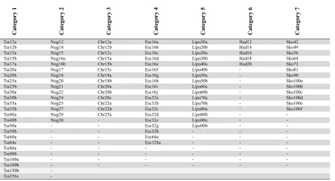
Table 1
Instances of QAP from QAPLIB
C
at
eg
or
y
1
C
at
eg
or
y
2
C
at
eg
or
y
3
C
at
eg
or
y
4
C
at
eg
or
y
5
C
at
eg
or
y
6
C
at
eg
or
y
7
Tai12a Nug12 Chr12a Esc16a Lipa20a Had12 Sko42
Tai12b Nug14 Chr12b Esc16b Lipa20b Had14 Sko49
Tai15a Nug15 Chr12c Esc16c Lipa30a Had16 Sko56
Tai15b Nug16a Chr15a Esc16d Lipa30b Had18 Sko64
Tai17a Nug16b Chr15b Esc16e Lipa40a Had20 Sko72
Tai20a Nug17 Chr15c Esc16f Lipa40b - Sko81
Tai20b Nug18 Chr18a Esc16g Lipa50a - Sko90
Tai25a Nug20 Chr18b Esc16h Lipa50b - Sko100a
Tai25b Nug21 Chr20a Esc16i Lipa60a - Sko100b
Tai30a Nug22 Chr20b Esc16j Lipa60b - Sko100c
Tai30b Nug24 Chr20c Esc32a Lipa70a - Sko100d
Tai35a Nug25 Chr22a Esc32b Lipa70b - Sko100e
Tai35b Nug27 Chr22b Esc32c Lipa80a - Sko100f
Tai40a Nug28 Chr25a Esc32d Lipa80b - -
Tai40b Nug30 - Esc32e Lipa90a - -
Tai50a - - Esc32g Lipa90b - -
Tai50b - - Esc32h - - -
Tai60a - - Esc64a - - -
Tai64c - - Esc128a - - -
Tai80a - - - -
Tai80b - - - -
Tai100a - - - -
Tai100b - - - -
Tai150b -
Tai256c -
5.1 Parameter setting
In order to determine the most appropriate parameter settings, extensive experiments, as well as many runs of the algorithm, were performed. The set values of the parameters for the three algorithms were presented in Table 2. The quality of the solutions obtained by using the proposed algorithm can be influenced by the set algorithm parameters. To identify the most suitable set of parameter values that produce desirable outcomes, numerous tests were performed.
Table 2
Parameter setting
Parameter Value
NP Number of Population 200
Maximum Iterations 100
Pm Perturbation Probability of Mutation 0.7
Pc Perturbation Probability of Crossover 0.8
Ph Probability of Hybrid 0.5
Maximum waiting for solutions updates 10
Tabu list length 10
Maximum iterations of TS 25
Number of runs 10
5.2 Results and Discussions
algorithm which is proposed in this study HDDETS was evaluated by comparing it with other algorithms. Specific criteria which include quality of solution and measured running times were used in comparing the algorithms. The use of quality of solution criterion for comparison of algorithms is more appropriate in heuristic and estimation methods, especially (in optimization). On the other hand, the running time comparison criterion is the most appropriate for exact algorithms. However, in a case where the produced solutions are similar in terms of quality, comparison of running times of approximation algorithms and heuristics will be suitable. This work focused on solution quality. The accuracy of an algorithm is calculated using a percentage deviation or gap. In this study, the solution quality criterion was used in calculating the accuracy, which is calculated through the question below:
Gap = (CBest - C*) / C* ×100, (7)
where CBest is the best objective value found over 10 runs, while C* is the best-known value taken from
QAPLIB. The results of the proposed algorithm (HDDETS) are presented in Table 3. The results are discussed using three scenarios as follows:
Scenario 1:
The proposed algorithm was applied to the cases shown in Table 1. All the numerical results were excellent and have been presented in Table 3. It was found that the proposed algorithm achieved an accuracy of 100 % in 83 test instances out of 105 test instances. These excellent results can be attributed to the use of an algorithm feature that can continuously improve all the solutions in each iteration until the best solution is reached. The strength of this algorithm is due to the integration of the diversification property of the algorithm DDE with the intensification feature of TS algorithm, as well as the use of tabu-list which prevents the recurrence of solutions that have been visited in the past.
Results of the HDDETS algorithm for some instances from QAPLIB
N am e of p ro b le m S ol u ti on in Q A P L IB P ro po se d al go ri th m B es t So lu ti on W or st S ol ut io n A ve ra ge S ol u ti on B es t G ap W or st G ap A ve ra ge G ap T im e (s ec on d s) S ta nd er D iv is io n
Nug12 578 HDDETS 578 578 578 0 0 0 0.514 0
Nug14 1014 HDDETS 1014 1014 1014 0 0 0 0.432 0
Nug15 1150 HDDETS 1150 1150 1150 0 0 0 0.378 0
Nug16a 1610 HDDETS 1610 1610 1610 0 0 0 0.573 0
Nug16b 1240 HDDETS 1240 1240 1240 0 0 0 0.461 0
Nug17 1732 HDDETS 1732 1732 1732 0 0 0 4.204 0
Nug18 1930 HDDETS 1930 1930 1930 0 0 0 0.526 0
Nug20 2570 HDDETS 2570 2570 2570 0 0 0 1.889 0
Nug21 2438 HDDETS 2438 2438 2438 0 0 0 2.275 0
Nug22 3596 HDDETS 3596 3596 3596 0 0 0 1.672 0
Nug24 3488 HDDETS 3488 3488 3488 0 0 0 1.99 0
Nug25 3744 HDDETS 3744 3744 3744 0 0 0 3.201 0
Nug27 5234 HDDETS 5234 5234 5234 0 0 0 1.299 0
Nug28 5166 HDDETS 5166 5166 5166 0 0 0 43.434 0
Nug30 6124 HDDETS 6124 6148 6126 0 0.391 0.039 3.273 0.123
Chr12a 9552 HDDETS 9552 9552 9552 0 0 0 0.518 0
Chr12b 9742 HDDETS 9742 9742 9742 0 0 0 0.281 0
Chr12c 11156 HDDETS 11156 11156 11156 0 0 0 0.558 0
Chr15a 9896 HDDETS 9896 9896 9896 0 0 0 1.077 0
Chr15b 7990 HDDETS 7990 7990 7990 0 0 0 0.369 0
Chr15c 9504 HDDETS 9504 9504 9504 0 0 0 2.026 0
Chr18a 11098 HDDETS 11098 11098 11098 0 0 0 1.01 0
Chr18b 1534 HDDETS 1534 1534 1534 0 0 0 0.522 0
Chr20a 2192 HDDETS 2192 2192 2192 0 0 0 2.057 0
Chr20b 2298 HDDETS 2298 2298 2298 0 0 0 50.772 0
Chr20c 14142 HDDETS 14142 14142 14142 0 0 0 0.849 0
Chr22a 6156 HDDETS 6156 6156 6156 0 0 0 51.954 0
Chr22b 6194 HDDETS 6194 6194 6194 0 0 0 64.016 0
Results of the HDDETS algorithm for some instances from QAPLIB (Continued)
N am e of pr ob le m S ol ut io n in Q A P L IB P ro p os ed al go ri th m B es t S ol ut io n W or st S ol ut io n A ve ra ge S ol ut io n B es t G ap W or st G ap A ve ra ge G ap T im e (s ec on ds ) St an de r D iv is io n
Sko42 15812 HDDETS 15812 15818 15814 0 0.037 0.015 20.864 0.019
Sko49 23386 HDDETS 23386 23440 23403 0 0.23 0.072 27.001 0.063
Sko56 34458 HDDETS 34458 34580 34503 0 0.354 0.131 623.89 0.132
Sko64 48498 HDDETS 48498 48902 48622 0 0.833 0.255 858.975 0.241
Sko72 66256 HDDETS 66316 66626 66429 0.09 0.558 0.261 368.841 0.136
Sko81 90998 HDDETS 91060 91524 91313 0.068 0.578 0.346 1624.424 0.18
Sko90 115534 HDDETS 115756 116498 116046 0.192 0.834 0.443 1727.96 0.197
Sko100a 152002 HDDETS 152316 154014 152725 0.206 1.323 0.475 2969.776 0.382
Sko100b 153890 HDDETS 154168 155054 154600 0.18 0.756 0.461 1490.758 0.189
Sko100c 147862 HDDETS 148148 149426 148753 0.193 1.057 0.602 2930.167 0.325
Sko100d 149576 HDDETS 149762 150512 150217 0.124 0.625 0.428 1472.923 0.15
Sko100e 149150 HDDETS 149514 151034 150024 0.244 1.263 0.585 6488.738 0.341
Sko100f 149063 HDDETS 149714 150464 149919 0.454 0.958 0.592 1265.821 0.144
Tai12a 224416 HDDETS 224416 224416 224416 0 0 0 0.508 0
Tai12b 39464925 HDDETS 39464925 39464925 39464925 0 0 0 0.684 0
Tai15a 388214 HDDETS 388214 388214 388214 0 0 0 0.847 0
Tai15b 51765268 HDDETS 51765268 51765268 51765268 0 0 0 0.81 0
Tai17a 491812 HDDETS 491812 491812 491812 0 0 0 5 0
Tai20a 703482 HDDETS 703482 706786 704026 0 0.469 0.077 5.653 0.167
Tai20b 122455319 HDDETS 122455319 122455319 122455319 0 0 0 0.511 0
Tai25a 1167256 HDDETS 1167256 1174422 1170285 0 0.613 0.259 7.848 0.209
Tai25b 344355646 HDDETS 344355646 344355646 344355646 0 0 0 13.46 0
Tai30a 1818146 HDDETS 1818146 1818146 1818146 0 0 0 57.4 0
Tai30b 637117113 HDDETS 637117113 637117113 637117113 0 0 0 29.794 0
Tai35a 2422002 HDDETS 2422002 2431810 2423613 0 0.404 0.066 29.589 0.131
Tai35b 283315445 HDDETS 283315445 283315445 283315445 0 0 0 57.4 0
Tai40a 3139370 HDDETS 3141431 3151727 3148060 0.065 0.393 0.276 138.357 0.087
Tai40b 637250948 HDDETS 637250948 650062131 638532066 0 2.01 0.201 416.445 0.635
Tai50a 4938796 HDDETS 4989160 5010958 5002852 1.019 1.461 1.297 768.214 0.162
Tai50b 458821517 HDDETS 458821517 460726849 459656699 0 0.415 0.182 48.479 0.194
Tai60a 7205962 HDDETS 7281638 7338518 7309055 1.05 1.839 1.43 921.089 0.263
Tai60b 608,215,054 HDDETS 7205962 608501817 640242782 0.047 5.265 1.526 42.188 1.616
Tai64c 1855928 HDDETS 1855928 1855928 1855928 0 0 0 8.308 0
Tai80a 13499184 HDDETS 13642148 13749540 13690956 1.059 1.854 1.42 1195.736 0.215
Tai80b 818415043 HDDETS 818415043 831997039 824550128 0 1.659 0.749 1399.883 0.561
Tai100a 21125314 HDDETS 21269898 21395720 21342495 1.069 1.667 1.414 2740.755 0.202
Tai100b 1185996137 HDDETS 1187179912 1212182931 1191632007 0.099 2.208 0.475 1553.481 0.624
Tai150b 498896643 HDDETS 501892435 508173332 505261057 0.6 1.859 1.275 9402.76 0.442
Tai256c 44759294 HDDETS 44786418 44838798 44813276 0.06 0.177 0.12 41014.57 0.041
Esc16a 68 HDDETS 68 68 68 0 0 0 0.533 0
Esc16b 292 HDDETS 292 292 292 0 0 0 0.634 0
Esc16c 160 HDDETS 160 160 160 0 0 0 0.577 0
Esc16d 16 HDDETS 16 16 16 0 0 0 0.532 0
Esc16e 28 HDDETS 28 28 28 0 0 0 0.55 0
Esc16f 0 HDDETS 0 0 0 0 0 0 0.426 0
Esc16g 26 HDDETS 26 26 26 0 0 0 0.472 0
Esc16h 996 HDDETS 996 996 996 0 0 0 0.473 0
Esc16i 14 HDDETS 14 14 14 0 0 0 0.629 0
Esc16j 8 HDDETS 8 8 8 0 0 0 0.737 0
Esc32a 130 HDDETS 130 130 130 0 0 0 7.953 0
Esc32b 168 HDDETS 168 168 168 0 0 0 1.924 0
Esc32c 642 HDDETS 642 642 642 0 0 0 2.276 0
Esc32d 200 HDDETS 200 200 200 0 0 0 2.184 0
Esc32e 2 HDDETS 2 2 2 0 0 0 1.835 0
Esc32g 6 HDDETS 6 6 6 0 0 0 1.907 0
Esc32h 438 HDDETS 438 438 438 0 0 0 1.896 0
Esc64a 116 HDDETS 116 116 116 0 0 0 9.927 0
Results of the HDDETS algorithm for some instances from QAPLIB (Continued)
N am e of pr ob le m S ol ut io n in Q A P L IB P ro p os ed al go ri th m B es t S ol ut io n W or st S ol ut io n A ve ra ge S ol ut io n B es t G ap W or st G ap A ve ra ge G ap T im e (s ec on ds ) St an de r D iv is io n
Lipa20a 3683 HDDETS 3683 3683 3683 0 0 0 1.351 0
Lipa20b 27076 HDDETS 27076 27076 27076 0 0 0 1.011 0
Lipa30a 131178 HDDETS 131178 131178 131178 0 0 0 9.965 0
Lipa30b 151426 HDDETS 151426 151426 151426 0 0 0 5.141 0
Lipa40a 31538 HDDETS 31538 31844 31684 0 0.97 0.461 16.246 0.487
Lipa40b 476581 HDDETS 476581 476581 476581 0 0 0 6.946 0
Lipa50a 62093 HDDETS 62093 62629 62451 0 0.863 0.576 42.387 0.398
Lipa50b 1210244 HDDETS 1210244 1210244 1210244 0 0 0 32.891 0
Lipa60a 107218 HDDETS 107897 108019 107959 0.633 0.747 0.69 463.998 0.034
Lipa60b 2520135 HDDETS 2520135 2969956 2742733 0 17.849 8.832 433.066 9.311
Lipa70a 169755 HDDETS 170787 170858 170824 0.607 0.649 0.629 1056.769 0.014
Lipa70b 4603200 HDDETS 4603200 5475784 5285704 0 18.956 14.8267 470.74 7.818
Lipa80a 253195 HDDETS 254506 254695 254590 0.517 0.592 0.551 719.781 0.023
Lipa80b 7763962 HDDETS 7763962 9293826 9131465 0 19.7047 17.613 176.991 6.189
Lipa90a 360630 HDDETS 362307 362601 362480 0.465 0.546 0.513 2000.489 0.026
Lipa90b 12490441 HDDETS 12490441 15002587 14479768 0 20.112 15.926 1851.828 8.395
Had12 1652 HDDETS 1652 1652 1652 0 0 0 0.784 0
Had14 2724 HDDETS 2724 2724 2724 0 0 0 0.583 0
Had16 3720 HDDETS 3720 3720 3720 0 0 0 0.437 0
Had18 5358 HDDETS 5358 5358 5358 0 0 0 0.674 0
Had20 6922 HDDETS 6922 6922 6922 0 0 0 0.837 0
Scenario 2:
All solutions for all cases mentioned in the database of QAP are divided into two types:
Optimal Solution (OPT)
Best Known Solution (BKS)
In this study, the number of instances that have the Optimal Solution is 77 instances and the number of instances that have the Best-Known Solution is 28 instances. An Optimal Solution can be obtained by the proposed algorithm in 73 instances out of 77 instances and it can produce Best Known Solution in 10 instances out of 28 instances. The first comparison was done in this study to evaluate the effectiveness of the proposed algorithm HDDETS. The proposed algorithm was compared with TS and DDE. In Table 4, the results of the comparison are presented, and it can be observed from the results that the HDDETS outperformed DDE and TS in all instances. Afterward, another comparison has been carried out between the proposed algorithm and another algorithm in the literature. Prior to the proposal of a hybrid algorithm in this study, a new approach called whale algorithm integrated with Tabu search for quadratic assignment problem (WAITS) had been introduced by (Abdel-Basset et al., 2018a). A comparison was done between the WAITS and the algorithm proposed in this study. Based on the outcome of the comparison, the performance of WAITS is better than that of other algorithms in terms of solving QAP. More so, it can produce an optimal solution for many instances of QAP.
Table 4 shows the comparison between our proposed HDDETS and WAITS. The main contribution of this study is providing an improved solution for QAP, especially that which has not produced an optimal solution. For instance, in the case of (Tai50a, Tai80b, Tai100a, and Tai150b) the best gap of this instance
was reached at (1.57 %, 1.20 %, 2.04 %, and 1.76 %respectively) compared with the solution in a dataset
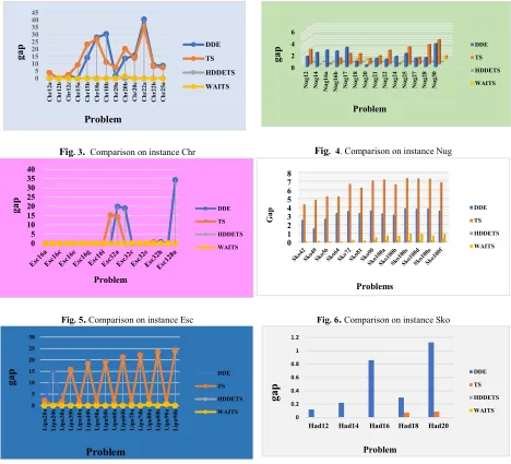
to improve the solutions of these instances so that they can reach the best or the same values within the database for QAP. So far, the best gap has been found for these cases by WAITS as follows: (0.13 %, 0.08 %, 0.07 %, 0.27 %, 0.74 %, and 0.76 %, respectively). Another contribution of the algorithm HDDETS is enhancing the solutions of these instances; the results produced by HDDETS were found to be better than those of WAITS. More so, HDDETS reached the best gap of (0 %, 0 %, 0 %, 0.09 %, 0.18 %, and 0.124 %, respectively). Below are the figures (Figs. 3-9) that show the gaps obtained from the algorithms in Table 4. In Table 5 below, a summary of the comparison results between HDDETS and WAITS is presented.
Comparative results between DDE, TS, HDDETS, and WAITS algorithms for QAP
No. Problem Best-Known
Solution DDE TS HDDETS WAITS
Best gap Best gap Best gap Best gap
1 Chr12a 9552 0 3.810 0 0
2 Chr12b 9742 0 0 0 0
3 Chr12c 11156 2.312 2.312 0 0
4 Chr15a 9896 0 9.256 0 0
5 Chr15b 7990 14.167 23.329 0 0
6 Chr18a 11098 27.967 26.872 0 0
7 Chr18b 1534 30.365 11.155 0 0
8 Chr20a 2192 1.825 7.561 0 0
9 Chr20b 2298 13.594 20.255 0 1.56
10 Chr20c 14142 15.665 13.838 0 0
11 Chr22a 6156 40.347 35.384 0 0.16
12 Chr22b 6194 9.096 8.219 0 0
13 Chr25a 3796 8.653 7.426 0 0
14 Esc16a 68 0 0 0 0
15 Esc16b 292 0 0 0 0
16 Esc16c 160 0 0 0 0
17 Esc16d 16 0 0 0 0
18 Esc16e 28 0 0 0 0
19 Esc16f 0 0 0 0 0
20 Esc16g 26 0 0 0 0
21 Esc16h 996 0 0 0 0
22 Esc16i 14 0 0 0 0
23 Esc16j 8 0 15.3846 0 0
24 Esc32a 130 20 14.2857 0 0
25 Esc32b 168 19.047 0 0 0
26 Esc32c 642 0 0 0 0
27 Esc32d 200 0 0 0 0
28 Esc32e 2 0 0 0 0
29 Esc32g 6 0 0.91324 0 0
30 Esc32h 438 0.913 0 0 0
31 Esc64a 116 0 0 0 0
32 Esc128a 64 34.375 0 0 0
33 Lipa20a 3683 1.710 2.1721 0 0
34 Lipa20b 27076 14.791 0 0 0
35 Lipa30a 131178 1.844 1.7529 0 0
36 Lipa30b 151426 15.766 15.7998 0 0
37 Lipa40a 31538 1.417 1.4554 0 0
38 Lipa40b 476581 19.009 18.2678 0 0
39 Lipa50a 62093 1.3673 1.3705 0 0
40 Lipa50b 1210244 19.278 19.2295 0 0
41 Lipa60a 107218 1.221 1.2759 0.633 0
42 Lipa60b 2520135 21.013 21.2654 0 0
43 Lipa70a 169755 1.122 1.1611 0.607 0
44 Lipa70b 4603200 22.022 22.1949 0 0
45 Lipa80a 253195 1.029 1.0861 0.517 0.55
46 Lipa80b 7763962 23.047 23.4897 0 0
47 Lipa90a 360630 0.963 1.0559 0.465 0.50
Comparative results between DDE, TS, HDDETS, and WAITS algorithms for QAP (Continued)
No. Problem Best-Known Solution
DDE TS HDDETS WAITS
Best gap Best gap Best gap Best gap
49 Nug12 578 1.73 2.422 0 0
50 Nug14 1014 2.366 0 0 0
51 Nug16a 1150 2.782 0.173 0 0
52 Nug16b 1610 2.608 0.993 0 0
53 Nug17 1240 3.225 1.774 0 0
54 Nug18 1930 0.923 1.732 0 0
55 Nug20 2570 0.310 0.932 0 0
56 Nug21 2438 1.400 1.4 0 0
57 Nug22 3596 1.230 2.297 0 0
58 Nug24 3488 1.724 0.166 0 0
59 Nug25 3744 2.216 2.867 0 0
60 Nug27 5234 1.442 1.121 0 0
61 Nug28 5166 1.528 3.248 0 0
62 Nug30 6124 3.832 4.065 0 0.52
63 Sko42 15812.0 2.567 4.3638 0 0
64 Sko49 23386 1.599 4.8833 0 0.13
65 Sko56 34458 2.704 5.2876 0 0.08
66 Sko64 48498 3.365 5.2909 0 0.07
67 Sko72 66256 3.595 6.7164 0.09 0.27
68 Sko81 90998 3.356 6.2815 0.068 0.19
69 Sko90 115534 3.661 7.1183 0.192 0.56
70 Sko100a 152002 3.326 7.2039 0.206 0.76
71 Sko100b 153890 3.184 6.6723 0.18 0.74
72 Sko100c 147862 3.907 7.3799 0.193 0.99
73 Sko100d 149576 3.866 7.3394 0.124 0.98
74 Sko100e 149150 3.886 7.3067 0.244 0.76
75 Sko100f 149036 3.616 6.899 0.454 0.95
76 Had12 1652 0.121 0 0 0
77 Had14 2724 0.22 0 0 0
78 Had16 3720 0.86 0 0 0
79 Had18 5358 0.298 0.074 0 0
80 Had20 6922 1.126 0.086 0 0
81 Tai12a 224416 0 3.842 0 0
82 Tai12b 39464925 2.8496 4.263 0 0
83 Tai15a 388214 2.043 0.16898 0 0
84 Tai15b 51765268 0.339 2.4024 0 0
85 Tai20a 491812 2.983 0.90165 0 0
86 Tai20b 703482 4.592 4.3505 0 0
87 Tai25a 122455319 1.743 1.6315 0 0
88 Tai25b 1167256 4.216 4.0909 0 0
89 Tai30a 344355646 2.039 6.5651 0 0.48
90 Tai30b 1818146 4.548 5.5332 0 0
91 Tai35a 637117113 3.502 4.0868 0 0.06
92 Tai35b 2422002 4.777 6.3761 0 0
93 Tai40a 3139370 2.157 0.092568 0 0.52
94 Tai40b 637250948 4.748 6.9324 0.065 0.005
95 Tai50a 637250948 0.0769 11.4704 0 1.57
96 Tai50b 4938796 5.246 12.7767 1.019 0.05
97 Tai60a 458821517 3.388 13.2447 0 1.93
98 Tai60b 7205962 4.609 1.974 0.047 0.74
99 Tai64c 1855928 0.4175 2.4024 0 0
100 Tai80a 13499184 5.665 0.90165 1.059 1.90
101 Tai80b 818415043 7.486 4.3505 0 1.20
102 Tai100a 21125314 5.743 1.6315 1.146 2.04
103 Tai100b 1185996137 7.116 4.0909 0.099 0.50
104 Tai150b 498896643 8.6079 6.5651 0.6 1.76
Below the figures which show the gaps obtained from the performance of the algorithms in Table 4.
Fig. 2. comparison among DDE, TS, HDDETS, and WAITS
Fig. 3. Comparison on instance Chr Fig. 4. Comparison on instance Nug
Fig. 5. Comparison on instance Esc Fig. 6. Comparison on instance Sko
Fig. 7. Comparison on instance Lipa Fig. 8. Comparison on instance Lipa
DDE TS HDDETS WAITS
5.207 5.265 0.069 0.178 A ve ra ge b es t ga p Methods 0 5 10 15 20 25 30 35 40 45 C h r1 2a C h r1 2b C h r1 2c C h r1 5a C h r1 5b C h r1 8a C h r1 8b C h r2 0a C h r2 0b C h r2 0c C h r2 2a C h r2 2b C h r2 5a ga p Problem DDE TS HDDETS WAITS 0 2 4 6 N u g1 2 N u g1 4 N u g1 6a N u g1 6b N u g1 7 N u g1 8 N u g2 0 N u g2 1 N u g2 2 N u g2 4 N u g2 5 N u g2 7 N u g2 8 N u g3 0 ga p Problem DDE TS HDDETS WAITS 0 5 10 15 20 25 30 35 40 ga p Problem DDE TS HDDETS WAITS 0 1 2 3 4 5 6 7 8 G ap Problems DDE TS HDDETS WAITS 0 5 10 15 20 25 30 L ip a2 0a L ip a2 0b L ip a3 0a L ip a3 0b L ip a4 0a L ip a4 0b L ip a5 0a L ip a5 0b L ip a6 0a L ip a6 0b L ip a7 0a L ip a7 0b L ip a8 0a L ip a8 0b L ip a9 0a L ip a9 0b ga p Problem DDE TS HDDETS WAITS 0 0.2 0.4 0.6 0.8 1 1.2
Had12 Had14 Had16 Had18 Had20
Fig. 9. Comparison on instance Tai
Table 5 presents a summary of the comparison results between HDDETS and WAITS.
Summary of the comparison results between HDDETS and WAITS
Category Name of Problem
Number of Instances
Type of Solution HDDETS WAITS
OPT BKS OPT BKS OPT BKS
1 Tai 25 10 15 10 7 8 3
2 Nug 14 14 - 14 - 13 -
3 Chr 13 13 - 13 - 11 -
4 Esc 19 19 - 19 - 19 -
5 Lipa 16 16 - 12 - 14 -
6 Had 5 5 - 5 - 5 -
7 Sko 13 - 13 - 3 - 1
Sum 105 77 28 73 10 70 4
Scenario 3:
In the next step, the effect and validation of the proposed algorithm HDDETS are presented. This is achieved by comparing the proposed algorithm with other algorithms. The most robust and latest algorithms were used for the comparison. Table 6 shows the results of the comparison between HDDETS and four other algorithms. Comparisons between HDDETS and the following algorithms were done:
Discrete Bat Algorithm (DBA) (Riffi et al., 2017)
Development of modified discrete particle swarm (DPSO) (Pradeepmon, 2018)
Biogeography-Based Optimization Algorithm Hybridized with Tabu Search (BBOTS) (Lim et
al., 2016)
A hybrid algorithm combining lexisearch and genetic algorithms (LSGA) (Ahmed, 2018)
For the compared cases in Table 6, the first comparison which was between HDDETS and DBA, it was found that the DBA can reach the optimal solution for 35 out of 54 instances and reach to Best Known Solution for 5 out of 21 instances. While the HDDETS has been solved 54 optimal solutions out of 54 instances, this implies that the gap of the best value found was 0 %. On another hand, it was observed that the HDDETS can reach the Best-Known Solution for 12 out of 21 instances. The results obtained by the DBA algorithm are as follows: the optimal solution was achieved for (8 instances from case Bur out of 8 instances, 5 instances from the case Chr out of 5 instances, 10 instances from the case Esc out of 10 instances, 3 instances from the case Nug out of 15 instances, and 9 instances from the case Tai out of 10). For the best-known solution in case Tai, the DBA can reach 4 instances out of 14 instances, the best
0 2 4 6 8 10 12 14
value for the best average gap report is 0.872 %. HDDETS can found 8 best-known solutions out of 14 instances with the best value is 0.333 % of the average gap. Next test for the best-known solution has been applied on a case Sko, the results show DBA found 1 best-known solution out for 7 instances with the best average gap value is 0.208 %. Whereas HDDETS has been reached to 4 best-known solutions out for 7 instances and the best average gap is 0.05 %.
The next comparison was between HDDETS and DPSO; DPSO has been tested on 23 instances of QAP which produced optimal solutions. The results have shown that one optimal solution was found, and the results recorded the best value for an average gap for the rest of the instances at 0.618 %. When the HDDETS was applied to these instances, it was found that HDDETS has the capability of improving all the 23 instances, while reducing the gap to 0 % for all these instances. Similarly, the proposed algorithm has been compared with BBOTS, and this algorithm was applied in 5 cases (Bur, Chr, Esc, Nug, and Tai) of QAP. The results of these comparisons are as follows: in the case of Bur, the best value of the average gap was found to be 0.003 %. On the other hand, results obtained from the proposed algorithm HDDETS achieved an average gap of 0 %. For cases Chr, the difference between the results was obvious, where the performance of HDDETS was better than BBOTS; the average gap obtained by HDDETS was 0.185 %, while the best average gap was 0 %. The results of the comparison were equal to an average gap for both BBOTS and HDDETS algorithms in case Esc. For the case of Nug, the results for BBOTS in terms of the best value for the average gap was 0.019 %, while it was found that the HDDETS can lower the average gap to 0 %. On the other hand, for instances (tai12a, tai15a, tai17a, tai20a, tai30a, and tai80a) the BBOTS algorithm was used to solve these cases, and the average gap of 0.892 % was achieved, while the use of HDDETS to solve these instances enhanced the reduction of the best average rate to 0 %.
Comparison among DBA, DPSO, BBOTS, and HDDETS
No. Problem Type of Solve DBA DPSO BBOTS HDDETS
OPT BKS Best Solve Gap Best Solve
Gap Best Solve
Gap Best Solve Gap
1 bur26a 5,426,670 - 5,426,670 0 5434783 0.150 5426670 0.028 5,426,670 0
2 bur26b 3,817,852 - 3,817,852 0 3824420 0.172 3817852 0 3,817,852 0
3 bur26c 5,426,795 - 5,426,795 0 5428396 0.030 5426795 0 5,426,795 0
4 bur26d 3,821,225 - 3,821,225 0 3821419 0.005 3821225 0 3,821,225 0
5 bur26e 5,386,879 - 5,386,879 0 5387320 0.008 5386879 0 5,386,879 0
6 bur26f 3,782,044 - 3,782,044 0 3783123 0.029 3782044 0 3,782,044 0
7 bur26g 10,117,172 - 10,117,172 0 10118542 0.014 10117172 0 10,117,172 0
8 bur26h 7,098,658 - 7,098,658 0 7099677 0.014 7098658 0 7,098,658 0
9 chr12a 9552 - 9552 0 - - 9552 0 9552 0
10 chr12b 9742 - 7990 - - - 9742 0 9742 0
11 chr12c 11156 - - - 11156 0 11156 0
12 chr15a 9896 - - - 9896 0 9896 0
13 chr15b 7990 - - 0 - - 7990 0.298 7990 0
14 chr15c 9504 - - - 9504 0 9504 0
15 chr18a 11098 - 11,098 0 - - 11098 0.079 11098 0
16 chr18b 1534 - - - 1534 0 1534 0
17 chr20a 2192 - - - 2192 0.876 2192 0
18 chr20c 14142 - 14,142 0 - - 14142 0.604 14142 0
19 chr25a 3796 - 3796 0 - - - - 3796 0
20 esc16a 68 - 68 0 - - 68 0 68 0
21 esc16b 292 - 292 0 - - 292 0 292 0
22 esc16c 160 - 160 0 - - 160 0 160 0
23 esc16d 16 - 16 0 - - - - 16 0
24 esc16e 28 - 28 0 - - - - 28 0
25 esc16f 0 - 0 0 - - - - 0 0
26 esc32a 130 - 130 0 - - - - 130 0
27 esc32e 2 - 2 0 - - - - 2 0
28 esc32g 6 - 6 0 - - - - 6 0
Comparison among DBA, DPSO, BBOTS, and HDDETS (Continued)
No. Problem Type of Solve DBA DPSO BBOTS HDDETS
OPT BKS Best Solve Gap Best
Solve Gap Solve Best Gap Best Solve Gap
30 nug12 578 - - - 582 0.692 578 0 578 0
31 nug14 1014 - - - 1016 0.197 1014 0 1014 0
32 nug15 1150 - - - 1164 1.217 1150 0 1150 0
33 nug16a 1610 - - - 1630 1.242 1610 0 1610 0
34 nug16b 1240 - - - 1240 0.000 1240 0 1240 0
35 nug17 1732 - - - 1750 1.039 1732 0.012 1732 0
36 nug18 1930 - - - 1936 0.311 1930 0 1930 0
37 nug20 2570 - 2570 0 2570 0 2570 0 2570 0
38 nug21 2438 - 2438 0 2444 0.246 2438 0 2438 0
39 nug22 3596 - - - 3602 0.167 3596 0 3596 0
40 nug24 3488 - - - 3578 2.580 3488 0 3488 0
41 nug25 3744 - - - 3766 0.588 3744 0 3744 0
42 nug27 5234 - - - 5294 1.146 5234 0 5234 0
43 nug28 5166 - - - 5228 1.200 5166 0.209 5166 0
44 nug30 6124 - 6124 0 6206 1.339 6124 0.065 6124 0
45 tai12a 224,416 - 224,416 0 - - 224416 0 224416 0
46 tai12b 39,464,925 - 39,464,925 0 - - - - 39464925 0
47 tai15a 388,214 - 388,214 0 - - 388214 0 388214 0
48 tai15b 51,765,268 - 51,765,268 0 - - - - 51765268 0
49 tai17a 491,812 - 491,812 0 - - 491812 0.093 491812 0
50 tai20a 703,482 - 703,482 0 - - 705622 0.677 703482 0
51 tai20b 122,455,319 - 122,455,319 0 - - - - 122455319 0
52 tai25a 1,167,256 - 1,172,754 0.47 - - - - 1167256 0
53 tai25b 344,355,646 - 344,355,646 0 - - - - 344355646 0
54 tai30a - 1,818,146 1,831,272 0.72 - - 1843224 1.795 1818146 0
55 tai30b 637,117,113 - 637,117,113 0 - - - - 637117113 0
56 tai35a - 2,422,002 2,438,440 0.67 - - - - 2422002 0
57 tai35b - 283,315,445 283,315,445 0 - - - - 283315445 0
58 tai40a - 3,139,370 3,139,370 1.3 - - - - 3150391 0
59 tai40b - 637,250,948 637,250,948 0 - - - - 637250948 0.065
60 tai50a - 4,938,796 5,042,654 2.10 - - - - 4965748 0
61 tai50b - 458,821,517 458,830,119 0 - - - - 458821517 1.019
62 tai60a - 7,205,962 7,387,482 2.5 - - - - 7266970 0
63 tai60b - 608,215,054 608,414,385 0.03 - - - - 1855928 1.05
64 tai64c - 1,855,928 1,855,928 0 - - - - 13616880 0
65 tai80a - 13,499,184 13,810,130 2.30 - - 13841214 2.788 818415043 1.059
66 tai80b - 818,415,043 819,367,807 0.11 - - - - 818415043 0
67 tai100a - 21,052,466 21,541,326 2.3 - - - - 21285950 1.146
68 tai100b - 1185996137 1188168753 0.18 - - - - 1187179912 0.099
69 sko42 - 15,812 15,812 0 - - - - 15812 0
70 sko49 - 23,386 23,421 0.14 - - - - 23386 0
71 sko56 - 34,458 34,524 0.19 - - - - 34458 0
72 sko64 - 48,498 48,656 0.32 - - - - 48498 0
73 sko72 - 66,256 66,422 0.25 - - - - 66256 0.09
74 sko81 - 90,998 91,252 0.27 - - - - 91008 0.068
75 sko90 - 115,534 115,874 0.29 - - - - 115578 0.192
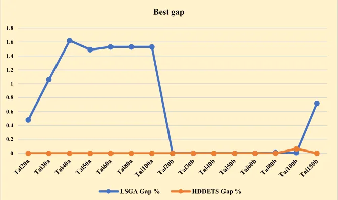
Comparison among LSGA and HDDETS
Instance BKS LSGA HDDETS Instance BKS LSGA HDDETS
Gap % Gap % Gap % Gap %
Tai20a 703,482 0.48 0 sko42 15,812 0 0
Tai30a 1,818,146 1.06 0 sko49 23,386 0.14 0
Tai40a 3,139,370 1.62 0 sko81 90,998 0.1 0.068
Tai50a 4,938,796 1.49 0 sko90 115,534 0.33 0.192
Tai60a 7,205,962 1.53 0 sko100a 152,002 0.26 0.206
Tai80a 13,499,184 1.53 0 - - - -
Tai100a 21,052,466 1.53 0 - - - -
Tai20b 122,455,319 0 0 - - - -
Tai30b 637,117,113 0 0 - - - -
Tai40b 637,250,948 0 0 - - - -
Tai50b 458,821,517 0 0 - - - -
Tai60b 608,215,054 0 0 - - - -
Tai80b 818,415,043 0.01 0 - - - -
Tai100b 1,185,996,137 0.01 0.065 - - - -
Tai150b 498,896,643 0.72 0 - - - -
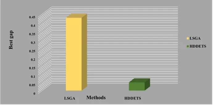
AVERAGE gap 0.665 0.004 0.191 0.093
Below Figures have been shown the gaps obtained from the performance of the algorithms in Table 7.
Fig. 10. Comparative study 1 between LSGA and HDDETS
Fig. 11. Comparative study 2 between LSGA and HDDETS 0
0.2 0.4 0.6 0.8 1 1.2 1.4 1.6 1.8
Best gap
LSGA Gap % HDDETS Gap %
0 0.05 0.1 0.15 0.2 0.25 0.3 0.35
sko42 sko49 sko81 sko90 sko100a
Best gap
Fig. 12. Comparison on Average best for QAP
6. Conclusion
In this paper, a Discrete Differential Evolution algorithm hybrid with Tabu Search HDDETS has been proposed with the aim of enhancing the solution of QAP. The limitation of the standard Discrete Differential Evolution algorithm is the low level of accuracy of solutions obtained for QAP problems, and this limitation has been alleviated by the proposed approach. The comparative results have shown that HDDETS algorithm outperforms the classic DDE and TS. The HDDETS algorithm has enhanced the solutions of QAP. Seven different case studies including 105 instances have been tested and used in analyzing the performance of the proposed HDDETS. The effect of the HDDETS algorithm on improving solutions was clear and has been discussed in the results and discussions section of this paper. The results showed the contribution of HDDETS to improving solutions of QAP. The HDDETS produced 73 optimal solutions out of 77 and has reached up to 10 best-known solutions out of 28. These are the best values obtained by the HDDETS compared to other recently proposed algorithms in the literature review in this paper. It is recommended that future research focus on the application of HDDETS algorithm in a real-world application such as Campus Layout or Hospital Layout. Another future work can focus on applying our proposed algorithm in other combinatorial optimization problems such as scheduling models or vehicle routing problem.
Acknowledgment
The authors would like to thanks to the Faculty of Information and Communication Technology, Centre for Research and Innovation Management, Universiti Teknikal Malaysia Melaka (UTeM) for providing the facilities and other support for this study.
References
Abdel-Baset, M., Wu, H., Zhou, Y., & Abdel-Fatah, L. (2017). Elite opposition-flower pollination algorithm for quadratic assignment problem. Journal of Intelligent & Fuzzy Systems, 33(2), 901-911.
Abdel-Basset, M., Manogaran, G., Rashad, H., & Zaied, A. N. H. (2018a). A comprehensive review of quadratic assignment problem: variants, hybrids and applications. Journal of Ambient Intelligence and
Humanized Computing, 1-24. doi: 10.1007/s12652-018-0917-x.
0 0.05 0.1 0.15 0.2 0.25 0.3 0.35 0.4 0.45
LSGA HDDETS
B
es
t
ga
p
Methods
LSGA
Abdel-Basset, M., Manogaran, G., El-Shahat, D., & Mirjalili, S. (2018b). Integrating the whale algorithm with tabu search for quadratic assignment problem: a new approach for locating hospital departments. Applied Soft Computing, 73, 530-546.
Abdelkafi, O., Idoumghar, L., & Lepagnot, J. (2015). Comparison of two diversification methods to solve the quadratic assignment problem. Procedia Computer Science, 51, 2703-2707.
Ahmed, Z. H. (2018). A hybrid algorithm combining lexisearch and genetic algorithms for the quadratic assignment problem. Cogent Engineering, 5(1), 1423743.
Benlic, U., & Hao, J. K. (2013). Breakout local search for the quadratic assignment problem. Applied Mathematics and Computation, 219(9), 4800-4815.
Cela, E., Deineko, V., & Woeginger, G. J. (2018). New special cases of the Quadratic Assignment Problem with diagonally structured coefficient matrices. European journal of operational research, 267(3), 818-834.
Czapiński, M. (2013). An effective parallel multistart tabu search for quadratic assignment problem on CUDA platform. Journal of Parallel and Distributed Computing, 73(11), 1461-1468.
Tate, D. M., & Smith, A. E. (1995). A genetic approach to the quadratic assignment problem. Computers & Operations Research, 22(1), 73-83.
Doerner, K., Focke, A., & Gutjahr, W. J. (2007). Multicriteria tour planning for mobile healthcare facilities in a developing country. European Journal of Operational Research, 179(3), 1078-1096. Duman, E., Uysal, M., & Alkaya, A. F. (2012). Migrating Birds Optimization: A new metaheuristic
approach and its performance on quadratic assignment problem. Information Sciences, 217, 65-77. Taillard, É. (1991). Robust taboo search for the quadratic assignment problem. Parallel computing,
17(4-5), 443-455.
Harris, M., Berretta, R., Inostroza-Ponta, M., & Moscato, P. (2015, May). A memetic algorithm for the quadratic assignment problem with parallel local search. In 2015 IEEE congress on evolutionary computation (CEC) (pp. 838-845). IEEE.
Kaviani, M., Abbasi, M., Rahpeyma, B., & Yusefi, M. (2014). A hybrid tabu search-simulated annealing method to solve quadratic assignment problem. Decision Science Letters, 3(3), 391-396.
Koopmans, T. C., & Beckmann, M. (1957). Assignment problems and the location of economic activities. Econometrica: journal of the Econometric Society, 25(1), 53-76.
Kushida, J. I., Oba, K., Hara, A., & Takahama, T. (2012, November). Solving quadratic assignment problems by differential evolution. In The 6th International Conference on Soft Computing and Intelligent Systems, and The 13th International Symposium on Advanced Intelligence Systems(pp. 639-644). IEEE.
Lim, W. L., Wibowo, A., Desa, M. I., & Haron, H. (2016). A biogeography-based optimization algorithm hybridized with tabu search for the quadratic assignment problem. Computational intelligence and neuroscience, 2016, 27.
Lv, C. (2012, October). A hybrid strategy for the quadratic assignment problem. In 2012 International Conference on Information Management, Innovation Management and Industrial Engineering (Vol. 2, pp. 31-34). IEEE.
Kaviani, M., Abbasi, M., Rahpeyma, B., & Yusefi, M. (2014). A hybrid tabu search-simulated annealing method to solve quadratic assignment problem. Decision Science Letters, 3(3), 391-396.
Pan, Q. K., Tasgetiren, M. F., & Liang, Y. C. (2008). A discrete differential evolution algorithm for the permutation flowshop scheduling problem. Computers & Industrial Engineering, 55(4), 795-816. Pradeepmon, T., Sridharan, R., & Panicker, V. (2018). Development of modified discrete particle swarm
optimization algorithm for quadratic assignment problems. International Journal of Industrial Engineering Computations, 9(4), 491-508.
Pradeepmon, T. G., Panicker, V. V., & Sridharan, R. (2016). Parameter selection of discrete particle swarm optimization algorithm for the quadratic assignment problems. Procedia Technology, 25, 998-1005.
Said, G. A. E. N. A., Mahmoud, A. M., & El-Horbaty, E. S. M. (2014). A comparative study of
meta-heuristic algorithms for solving quadratic assignment problem. International Journal of Advanced
Computer Science and Applications (IJACSA), 5(1), 1–6.
Shariff, S. R., Moin, N. H., & Omar, M. (2012). Location allocation modeling for healthcare facility planning in Malaysia. Computers & Industrial Engineering, 62(4), 1000-1010.
Şahinkoç, M., & Bilge, Ü. (2018). Facility layout problem with QAP formulation under scenario-based uncertainty. INFOR: Information Systems and Operational Research, 56(4), 406-427.
Samanta, S., Philip, D., & Chakraborty, S. (2018). Bi-objective dependent location quadratic assignment problem: Formulation and solution using a modified artificial bee colony algorithm. Computers & Industrial Engineering, 121, 8-26.
Scalia, G., Micale, R., Giallanza, A., & Marannano, G. (2019). Firefly algorithm based upon slicing structure encoding for unequal facility layout problem. International Journal of Industrial Engineering Computations, 10(3), 349-360.
Shukla, A. (2015, May). A modified bat algorithm for the quadratic assignment problem. In 2015 IEEE
Congress on Evolutionary Computation (CEC) (pp. 486-490). IEEE.
Da Silva, G. C., Bahiense, L., Ochi, L. S., & Boaventura-Netto, P. O. (2012). The dynamic space allocation problem: Applying hybrid GRASP and Tabu search metaheuristics. Computers & Operations Research, 39(3), 671-677.
Syam, S. S., & Côté, M. J. (2010). A location–allocation model for service providers with application to not-for-profit health care organizations. Omega, 38(3-4), 157-166.
Tasgetiren, M. F., Pan, Q. K., Suganthan, P. N., & Dizbay, I. E. (2013, April). Metaheuristic algorithms for the quadratic assignment problem. In 2013 IEEE Symposium on Computational Intelligence in Production and Logistics Systems (CIPLS) (pp. 131-137). IEEE.
Van Luong, T., Melab, N., & Talbi, E. G. (2010, July). Parallel hybrid evolutionary algorithms on GPU. In IEEE Congress on Evolutionary Computation (pp. 1-8). IEEE.
Xia, X., & Zhou, Y. (2018). Performance analysis of ACO on the quadratic assignment problem. Chinese Journal of Electronics, 27(1), 26-34.
Zhang, Y., Berman, O., Marcotte, P., & Verter, V. (2010). A bilevel model for preventive healthcare facility network design with congestion. IIE Transactions, 42(12), 865-880.