for Still Image Interpolation
Samreen Abbas
Department of Mathematics,
University of the Punjab, Lahore, Pakistan [email protected]
Malik Zawwar Hussain Department of Mathematics,
University of the Punjab, Lahore, Pakistan [email protected]
Misbah Irshad
Department of Mathematics,
Lahore College for Women University Lahore, Pakistan [email protected]
Abstract
In this paper, an image interpolation scheme is designed for 2D natural images. A local support rational cubic spline with control parameters, as interpolatory function, is being optimized using Genetic Algorithm (GA). GA is applied to determine the appropriate values of control parameter used in the description of rational cubic spline. Three state-of-the-art Image Quality Assessment (IQA) models with traditional one are involved for comparison with existing image interpolation schemes and perceptual quality check of resulting images. The results show that the proposed scheme is better than the existing ones in comparison.
Key words: Image Quality Assessment (IQA), Still Image, Genetic Algorithm (GA), Interpolation, Rational B-spline.
1. Introduction
Since 1970s, several piecewise polynomials have been considered to investigate the problems related to interpolation in the field of image processing by numerous writers, among whom are Hou and Andrews (1978), Parker et al. (1983) and Keys (1981). Piecewise cubic convolution along with high order B-splines are the most popular image interpolation functions. As splines did not have any concern to realistic stochastic models of digital images, so they are considered as a perfect fit for image processing.
In this paper, a local support rational cubic spline with control parameter is presented to investigate problems related to still image interpolation. The rational spline is optimized using Genetic Algorithm (GA). GA is applied to determine the appropriate values of control parameters of rational cubic spline. To examine smooth and improved quality results of interpolated images three structure similarity based Image Quality Assessment (IQA) metrics with traditional one are exercised here.
Rest of the paper is arranged as follows. The process of construction of local support rational spline and its extended interpolatory functions is presented in Section 2. Optimal interpolation using GA is addressed in Section 3 and Section 4. Section 5 includes all the experimental results and assessments. Finally concluding remarks are made in Section 6.
2. Rational Cubic B-Spline
In this section the construction method of local support based rational spline presented by Gregory and Sarfraz (1990) is reviewed and extended, in some way, to its one and two dimensional interpolatory functions. Let be the given set data points defined over the interval where be the partition of A piecewise rational cubic function is defined over each sub interval
as:
(1)
where and be the tension parameters defined in each sub
interval . The rational cubic function (1) has the following interpolating
properties:
and (2)
where denotes the derivatives with respect to and are the first derivatives at the knots , . For each sub interval , the rational cubic function (1) can be written in the form
(3)
where the function are the rational basis functions and found to be non-negative for with ∑ and defined here as:
, ,
with co-efficient of interpolation which are defined as:
In order to construct local support basis for rational cubic B-spline representation, let us first review the method presented by Gregory and Sarfraz (1990). Let the additional knots
and be introduced on both sides the
interval with as control parameters defined on this extended partition. A rational cubic spline function , can be introduced, such that
{
(4)
On the remaining two intervals will have the rational cubic form defined as:
( )
( ) (5)
where the function are defined same as above. The requirement that the function is continuous up to second order, in particular at , and
, may satisfy the following properties:
(
) ( )
}
(6)
where
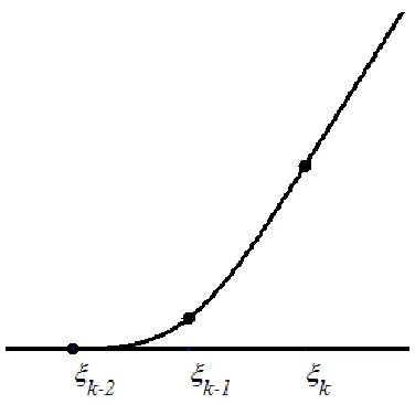
. The graphical view of the rational
Figure 1: The rational spline function
Now, to determine the local support basis for rational cubic spline, take the difference of
as:
(7)
where the function are themselves determined by getting the difference of the functions as:
( ) , (8)
with
(
) (
) ( ).
By the definition of the function in equation (8), it can be noticed that
{
(9)
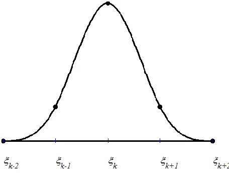
The graphical view of the rational cubic function is shown in Figure 2.
Therefore, an obvious representation of the rational cubic spline basis on an subinterval can be computed from equations (4) to equation (7) as:
( )
Figure 2: The rational spline function
where
for and
, ̂ ,
, ̂ ̂ ,
, ̂ , with
̂ , ̂ ,
̂ , ̂ .
The graphical view of the rational basis function , is shown in Figure 3.
Furthermore, both the 1–dimensional rational cubic B-spline and its extended 2-dimensional interpolatory functions will be formulated here using the local support basis (10). Let be the required rational spline interpolatory function defined as:
∑ (11)
where are coefficient of interpolation those can be determined from some set of discrete data at certain given spatial points. Substituting the value of from equation (10) in equation (11)
(12)
where
̂ ̂
̂ ( ̂ )
with
̂ ̂ ̂
̂ ̂
̂ .
So, the vector form of equation (12) can be presented as:
(13)
where
,
and with
[
̂
̂ ̂
̂ ]
.
Next, to extend the above one dimensional case to its two dimensions, equation (11) elaborates in the following expression
( ̃) ∑ ∑ ̃( ̃)
̃ [ ̃ ̃ (14)
̃ Finally, for , ̃ [ ̃ ̃ the function
( ̃) is vector form for 2- dimension rational spline is presented as:
( ̃) (15) with
,
[ ( ̃ ̃ ) ( ̃ ̃) ( ̃ ̃ ) ( ̃ ̃ )] ,
and the matrix is a corresponding extension of , defined as:
̃ (16) with
[
]
and is same as defined in equation (13) with corresponding extended matrix ̃.
3. Problem Optimization using Genetic Algorithms (GA)
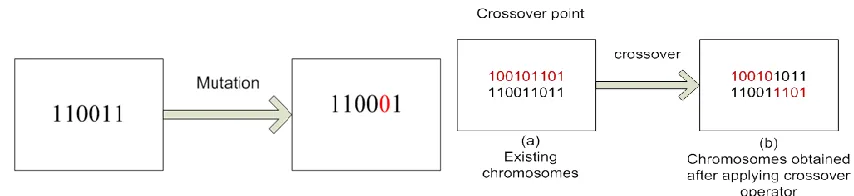
Genetic Algorithm (GA) is primitively suggested by Holland (1975). It represents a family of parallel adaptive search techniques. The techniques are based on the procedure of natural selection. GAs are practiced to produce globally optimized solutions in quick and effective way. Even in large solution spaces they perform outstandingly well as compared to other traditional optimization techniques. For survival in the large solution spaces GA strongly relies on three of its system operations; the selection, crossover and mutation. Through selection a pair of bit strings (parent bit strings) is chosen from the solution space or initial population which will further divided into two or more segments through the crossover operator. Crossover then combines these segments to produce new pair of bit strings (off springs) for next population. Mutation helps to reduce the possibility of GA to fall into local optimum. It carries out random changes in the slat of bit strings through the operations of bit shifting, rotation and inversion. Figure 4 illustrates both the crossover and mutation operators for some selected chromosomes (bunch of bit strings).
Since the this work is aimed to obtain an optimal solution for resulting interpolated images produced by using the rational cubic spline with control parameters and ̃ for
and , GA is used here to search for the appropriate values of control parameters. Now before starting the procedure for GA, several terms with system parameters are needed to be fixed in advance.
B. Objective Function: The proposed objective function is formulated by the sum square error which is defined for the image spatial data. For the original image spatial data metric and resulting image spatial data matrix , the proposed objective function is defined as:
( ̃) ∑ ∑ [ ( ̃ ) ] (17)
C. Stopping Criterion: The process will be stopped if no encouraging change in values of objective function is observed for a definite number of iterations.
Figure 4: Mutation and crossover operators for GA
4. Proposed Image Interpolation Scheme
An image interpolation scheme is designed using the rational cubic spline (15) with control parameters and ̃ for and , in its description. The scheme is made up of several steps which are elucidated here one by one. Firstly the spatial data of a selected original image is collected through any existing image decoding technique. In the next step, all the system parameters of GA are initialized to reach the optimized values of parameters and ̃ in the description of rational cubic spline (15). The initial population is taken randomly with potential compound of values of control parameters. Each control parameter corresponds to a single gene is a bit string or a chromosome. In the formulation if a gene is equal to 1, a value would be associated to the corresponding control parameter and if a gene is equal to 0, no value would be assigned to the corresponding control parameter. Successive implementation of GA search operations to the selected population, lead us to optimal values of and ̃ such that the fitness function (17) achieves its minimum value. Finally the spatial image data is interpolated using the optimized rational cubic spline.
5. Results and Discussion
into account. Therefore one should rely on subjective evolutions to evaluate the visual quality of resulting interpolated images. There are three natural photographical images: ‘Flower’, ‘Plane’ and ‘Pepper’ are used as reference/test images. All the images are 24-bit color images of size 512×512. Low resolution images with size 256×256 are obtained by direct down sampling the original reference images by a factor of two along each dimension. The low resolution images are up-sampled using the proposed image interpolation scheme to produce resulting interpolated images. The results produced by the proposed image interpolation scheme then compared with some representative work including Patch Based Non-Local (PB-NL) image interpolation introduced by Li (2008), New Edge-Directed Interpolation (NEDI) proposed by Li et al. (2001) and image Super Resolution algorithm based on Non-Local Means (SR-NLM) presented by Hung and Siu (2015).
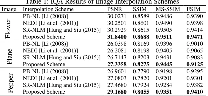
Table 1: IQA Results of Image Interpolation Schemes
Image Interpolation Scheme PSNR SSIM MS-SSIM FSIM
PB-NL [Li (2008)] 30.0271 0.8589 0.9486 0.9390
NEDI [Li et al. (2001)] 30.2501 0.8601 0.9490 0.9398
SR-NLM [Hung and Siu (2015)] 30.2929 0.8615 0.9505 0.9414
Proposed Scheme 31.8400 0.8688 0.9511 0.9471
PB-NL [Li (2008)] 26.0398 0.8169 0.9396 0.9010
NEDI [Li et al. (2001)] 26.2081 0.8198 0.9405 0.9065
SR-NLM [Hung and Siu (2015)] 26.7147 0.8203 0.9431 0.9083
Proposed Scheme 27.3358 0.8275 0.9445 0.9125
PB-NL [Li (2008)] 26.9601 0.7790 0.9198 0.9295
NEDI [Li et al. (2001)] 27.0803 0.7820 0.9201 0.9301
SR-NLM [Hung and Siu (2015)] 27.4680 0.7924 0.9284 0.9382
Proposed Scheme 29.1680 0.8055 0.9351 0.9410
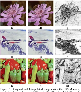
Table 1 depicts the PSNR, FSIM, SSIM and MS-SSIM values for all three colored natural image produced by using proposed image interpolation schemes and all three existing schemes are considered for comparison. From the outcomes shown in the table one can easily notice that the proposed scheme is better than the other interpolation schemes. Moreover, Figure 5 shows the SSIM map of ‘Flower’, ‘Plane’ and ‘Pepper’ with their original and resulting interpolated images.
6. Conclusion
A local support rational cubic spline with control parameter is investigated for problems related to still image interpolation. A soft computing technique, GA is utilized here to optimize rational spline. It helps find the appropriate values of respective control parameters. An image interpolation scheme is designed using the two dimensional optimal rational spline interpolatory function. FSIM, SSIM and MS-SSIM indices along with traditional PSNR are exercised to examine the quality of resulting interpolated images. The results show that our proposed interpolation scheme performs better as compared to the three existing schemes. The processing time for the images Flower, Plane and pepper in seconds are 34.415, 34.592 and 32.271 respectively in between two iterations of the proposed algorithm.
(a) (d) (g)
(b) (e) (h)
(c) (f) (i)
Figure 5: Original and Interpolated images with their SSIM maps, original reference images (a)‘Flower’, (b) ‘Plane’ and (c) ‘Pepper’, interpolated images (d) ‘Flower’, (e) ‘Plane’ and (f) ‘Pepper’, SSIM maps of the images (g) ‘Flower’, (h) ‘Plane’ and (i) ‘Pepper’.
References
1. Chang, P. H., Leou, J. J., Hsieh, H.C. (2001). A Genetic Algorithm Approach to Image Sequence Interpolation, Signal Processing: Image Communication, 16, 507-520.
2. Gregory, J. A., Sarfraz, M. (1990). A Rational Cubic Spline with Tension, Computer Aided Geometric Design, 7, 1-13.
3. Holland, J. H. (1975). Adaptation in Natural and Artificial Systems. MIT Press. 4. Hou, H. S., Andrews, H. C. (1978). Cubic Splines for Image Interpolation and
Digital Filtering, IEEE Transaction on Acoustics Speech and Signal Processing, 26(6), 508-517.
6. Jensen, K., Anastassiou, D. (1995). Sub-pixel Edge Localization and the Interpolation of Still Images, IEEE Transaction on Image Processing, 4 (3), 285-295.
7. Keys, R. G. (1981). Cubic Convolution Interpolation for Digital Image Processing, IEEE Transaction on Acoustics Speech and Signal Processing, 29(6), 1153-1160. 8. Kim, S. P., Su, W. Y. (1993). Recursive High-Resolution Reconstruction of Blurred
Multi Frame Images, IEEE Transaction on Image Processing, 2(4), 534-539.
9. Li, X. (2008). Patch-Based Image Interpolation: Algorithms and Applications, Proceeding International Workshop on Local and Non-Local Approximation in Image Processing, 1-6.
10. Li, X., Orchard, T. M. (2001). New Edge-Directed Interpolation, IEEE Transactions on Image Processing, 10(10), 1521-1527.
11. Parker, J. A., Kenyon, R. V., Troxel, D. V. (1983). Comparison of Interpolating Methods for Image Resampling, IEEE Transaction on Medical Imaging, MI-2 (1), 31-39.
12. Wang, Z., Bovik, A., Sheikh, H., Simoncelli, E. P. (2004). Image Quality Assessment: From Error Visibility to Structural Similarity, IEEE Transaction Image Processing, 3(4), 600-612.
13. Wang, Z., Simoncelli, E. P., Bovik, A. C. (2003). Multi-Scale Structural Similarity for Image Quality Assessment, Proceeding 37th IEEE Asilomar Conference on Signal, Systems and Computers, Pacific Grove, CA, Nov. 9-12.