Multifractal properties of embedded convective structures in orographic precipitation: toward subgrid-scale predictability

Nonlin. Processes Geophys., 20, 605–620, 2013 www.nonlin-processes-geophys.net/20/605/2013/ doi:10.5194/npg-20-605-2013

© Author(s) 2013. CC Attribution 3.0 License.

EGU Journal Logos (RGB)

Advances in

Geosciences

Open Access

Natural Hazards

and Earth System

Sciences

Annales

Geophysicae

Nonlinear Processes

in Geophysics

Atmospheric

Chemistry

and Physics

Atmospheric

Chemistry

and Physics

Atmospheric

Measurement

Techniques

Atmospheric

Measurement

Techniques

Biogeosciences

Open Access Open Access

Biogeosciences

Discussions

Climate

of the Past

Open Access Open Access

Climate

of the Past

Discussions

Earth System

Dynamics

Open Access Open Access

Earth System

Dynamics

Geoscientific

Instrumentation

Methods and

Data Systems

Open Access

Geoscientific

Instrumentation

Methods and

Data Systems

Geoscientific

Model Development

Open Access Open Access

Geoscientific

Model Development

Hydrology and

Earth System

Sciences

Hydrology and

Earth System

Sciences

Ocean Science

Open Access Open Access

Ocean Science

Solid Earth

Open Access Open Access

Solid Earth

The Cryosphere

Open Access Open Access

The Cryosphere

Natural Hazards

and Earth System

Sciences

Open Access

Discussions

Multifractal properties of embedded convective structures in

orographic precipitation: toward subgrid-scale predictability

M. Nogueira1,2, A. P. Barros2, and P. M. A. Miranda1

1_{Instituto Dom Luiz, University of Lisbon, Lisbon, Portugal}

2_{Pratt School of Engineering, Duke University, Durham, North Carolina, USA} Correspondence to: A. P. Barros (barros@duke.edu)

Received: 1 December 2011 – Revised: 9 April 2013 – Accepted: 29 July 2013 – Published: 11 September 2013

Abstract. Rain and cloud fields produced by fully

nonlin-ear idealized cloud resolving numerical simulations of oro-graphic convective precipitation display statistical multiscal-ing behavior, implymultiscal-ing that multifractal diagnostics should provide a physically robust basis for the downscaling and sub-grid scale parameterizations of moist processes. Our re-sults show that the horizontal scaling exponent function (and respective multiscaling parameters) of the simulated rainfall and cloud fields varies with atmospheric and terrain proper-ties, particularly small-scale terrain spectra, atmospheric sta-bility, and advective timescale. This implies that multifractal diagnostics of moist processes for these simulations are fun-damentally transient, exhibiting complex nonlinear behavior depending on atmospheric conditions and terrain forcing at each location. A particularly robust behavior found here is the transition of the multifractal parameters between stable and unstable cases, which has a clear physical correspon-dence to the transition from stratiform to organized (banded and cellular) convective regime. This result is reinforced by a similar behavior in the horizontal spectral exponent. Finally, our results indicate that although nonlinearly coupled fields (such as rain and clouds) have different scaling exponent functions, there are robust relationships with physical under-pinnings between the scaling parameters that can be explored for hybrid dynamical-statistical downscaling.

1 Introduction

It is often observed that air masses impinging upon a moun-tain range lead to the development of an orographic cloud with shallow embedded convective structures, which change the rainfall pattern and amount considerably, and can lead

to localized extreme values of rainfall. These localized ex-tremes present a great challenge for forecasters and are re-sponsible for mountain hazards including landslides, debris flows and flash floods.

The notion that embedded convective structures are the re-sult of exponential growth of small-scale disturbances in an unstable stratified layer (Kuo, 1963) motivated the applica-tion of linear stability analyses to gain insight on the dynam-ics of orographic convective precipitation, including the esti-mation of the unstable growth rate,ω, for each small-scale disturbance mode of wavenumber k=(kx, ky, kz) (Fuhrer and Schär, 2005):

ω= s

−N2 m

k2 x+k2y

k2_x+k2_y+k_z2 (1)

N_m2= 1 1+qw

0m

d dz

cp+clqwln(θe)

−

cl0mln(T )+g dqw

dz

(2) whereNmis the moist Brunt–Väisälä frequency of the satu-rated layer (as defined by Emanuel, 1994), which has a nega-tive value in the moist unstable case. In this inviscid formula-tion, the linear model predicts maximum growth for infinites-imally small horizontal wavelengths. Admitting that small-scale disturbances are ubiquitous in the real atmosphere, this does not agree with the observed finite spacing between bands observed in nature, e.g., in western Kyushu in Japan (Yoshizaki et al., 2000), in the Cévennes region in southern France (Miniscloux et al., 2001; Cosma et al., 2002) and the Oregon Coastal Range (Kirshbaum and Durran, 2005b; Kir-shbaum et al., 2007b). KirKir-shbaum et al. (2007a) developed a

new (also inviscid) linear model that includes an upstream stable region where stationary small-scale lee waves are triggered and subsequently used as the initial disturbances for the convective region. Their model agrees with the re-sults from numerical simulations that showed that such lee waves play a dominant role in triggering and organizing banded convection with finite spacing (Kirshbaum and Dur-ran, 2005a; Fuhrer and Schär, 2007). Using both linear stabil-ity analysis and idealized numerical simulations, additional factors were also found to be important such as (i) cloud depth (which determines the minimum value ofkz allowed in Eq. 1) (Kirshbaum and Durran, 2004); (ii) the advec-tive timescale, i.e., the in-cloud residence time of air parcels which can be controlled by mean wind speed and mountain width (Furher and Schär, 2005); (iii) dry stability outside the cloud layer (Kirshbaum and Durran 2005a); and (iv) cloud base height (Kirshbaum et al., 2007a).

A different approach to the problem has gradually devel-oped concurrent but separately in the last thirty years, where the (statistical) scaling behavior of physical processes is ex-plored. In these processes the statistical properties of a field at different scales are related by a scale-changing operation (generally a power law) that involves only the scale ratio and a scaling exponent, the simplicity of which is very appealing for statistical downscaling applications. In geophysical fields it is usually found that the scaling is determined not by one, but by an infinity of scaling exponents given by the scaling exponent function, i.e., they are multiscaling. Schertzer and Lovejoy (1987) proposed a functional form for this function, the universal multifractal (UM) model, briefly presented in Sect. 4. There are a number of publications reporting mul-tiscaling behavior in various geophysical fields, including cloud and rain fields, over various temporal (see e.g., de Lima and de Lima, 2009 for a review) and spatial ranges, e.g., Schertzer and Lovejoy (1987). Nykanen (2008) found scal-ing on horizontal maps of radar rain reflectivity; Gupta and Waymire (1993) found scaling on spatial fields of oceanic rainfall; Tessier et al. (1993) and Barros et al. (2004) found scaling in satellite-based fields of cloud radiances. Recently, Lovejoy et al. (2008a) looked at TRMM product 2A25 near surface reflectivity from rain measurements and found evi-dence of multiplicative cascades from planetary scales down to a few kilometers (∼4 km, the data set resolution) in the en-semble averaged scaling statistics. Also, note that the 2A25 product is an orbit based product with limited dimensions in the direction perpendicular to the satellite movement. They argued that the UM model with well posed fixed values of the scaling parameters is a good approach when considering the entire range of scales. Stolle et al. (2009) showed that data from global models (including ERA40 reanalysis and NOAA GFS) also accurately follow cascade statistics from nearly 20 000 km down to around 100 km, where there was a cut off by hyper viscosity of the numerical model linked to grid resolution.

However, there is no consensus on the specific values of the scaling exponents (and associated UM parameters) and scaling ranges in the literature, although some of the differ-ences might be attributed to sample size or differdiffer-ences in measurements (sensors, measurement methods or measure-ment errors, etc.). Another view is that the scaling exponents vary depending on contextual environmental conditions, and therefore the observed variations can be attributed in part to physical processes. Over and Gupta (1994) also used 2-D oceanic rainfall fields from GATE (GARP Atlantic Tropical Experiment), and proposed a relation between a scaling pa-rameter and large-scale average rain (argued to be an index of synoptic-scale weather conditions); Perica and Foufoula-Georgiou (1996) related scaling parameters computed from horizontal rainfall radar fields to the Convective Available Potential Energy (CAPE) of the pre-storm environment over the same area; Deidda (2000) and Deidda et al. (2004) also found a dependency in one of their scaling parameters com-puted from radar reflectivity on the large-scale mean rainfall rate; and more recently Nykanen (2008) linked the variation in the values of the multiscale statistical parameters com-puted from radar rainfall fields to the underlying topographic elevation, predominant orographic forcing and storm loca-tion, and movement relative to the orographic cross sections. These results suggest that UM parameters vary from event to event, or case study to case study as a function of atmospheric conditions, and local terrain parameters. If this behavior can be translated into robust relationships between UM parame-ters of particular states (e.g., precipitation) and the specific physical processes that determine the space-time evolution of these states (e.g., moist convection), then inference and induction modeling approaches can be used to develop quan-titative dynamical models of the state of interest relying on knowledge of the specific physical processes alone. For in-stance, to predict precipitation fields over a wide range of spatial scales knowing atmospheric stability conditions and precipitation at one (coarser) scale. This type of modeling could be used to formulate parameterizations of unresolved processes in numerical weather and climate prediction mod-els, and to predict states at spatial resolutions much finer than those resolved by models or observations, i.e., downscaling. In practical terms, this requires investigating possible rela-tionships between physical properties and statistical param-eters that would allow statistical downscaling from coarse to fine resolutions.

M. Nogueira et al.: Toward subgrid-scale predictability 607

profiles is investigated under different idealized climatologi-cal regimes (presented in Sect. 2), aiming to find physiclimatologi-cally based relationships between scaling parameters and atmo-spheric and terrain properties that can be estimated systemat-ically from coarser resolution simulations. The paper is orga-nized as follows: Sect. 2 presents the numerical setup; a sum-mary interpretation of the simulation results in light of the linear theories is presented in Sect. 3; and the empirical scal-ing analysis is presented in Sect. 4. The multifractal analysis based on the statistical moments and the UM model is briefly presented in Sect. 4.1. These methods are then applied to the simulations results and the variation of the scaling properties with simulation parameters is investigated for both 2-D rain and cloud fields (Sect. 4.2) and 3-D cloud fields (Sect. 4.3). The scaling in different fields is compared in Sect. 4.4. In Sect. 4.5, scaling analysis based on Fourier power spectra is performed on the 3-D cloud fields. The final section (Sect. 5) presents a summary and discussion of the main results.

2 Numerical simulations

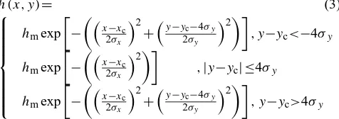
The numerical model Advanced Weather and Research Fore-casting (WRF-ARW) version 3.1 (Skamarock et al., 2008) is used to perform idealized cloud resolving simulations of conditionally unstable moist flow impinging upon a Gaussian shaped ridge (defined by Eq. 3), elongated on the cross-flow direction,y, and with a maximum terrain heighthm=600 m. When the flow is lifted by orography, it saturates and releases latent heat generating an unstable orographic cloud where the embedded convective structures will develop.

h (x, y)= (3)

       

      

hmexp

−

x−xc 2σx

2

+y−yc−4σy 2σy

2

, y−yc<−4σy hmexp

−

x−xc 2σx

2

,|y−yc| ≤4σy hmexp

−

x−xc 2σx

2

+y−yc−4σy 2σy

2

, y−yc>4σy Decay parameters σx and σy are 12.5 and 5 km, respec-tively, and the center of the ridge is defined at (xc, yc)= (80,60)km. The resulting modified Gaussian ridge is repre-sented in Fig. 1a. In all simulations the horizontal resolution is 250 m and there are 70 vertical terrain-following levels, un-equally distributed over the 15 km of the domain, with verti-cal spacing stretching from lower to higher levels in order to have better resolution in the region where orographic clouds will develop. A Rayleigh damping layer is introduced in the top 5 km to reduce spurious reflections at the top. To simplify the problem, the parameterizations for radiation or surface and boundary layer are turned off, and the effects of earth’s rotation are also neglected. The 3-D Smagorinsky scheme is used for sub-grid turbulence closure.

Fig. 1. Horizontal maps of topographic elevation (in meters) for simulations: (a) CTL and (b) Sst10km. The inner black square rep-resents the domain of interest where the scaling analysis computa-tions are performed.

disturbances in the domain reinforcing certain wavelengths, and would not allow the upstream stable flow to flow around the ridge, eventually forcing it all to transpose the orographic barrier.

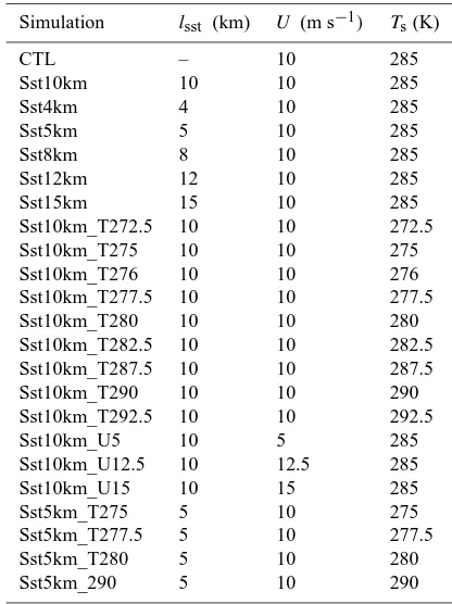
The upstream profiles are also highly idealized, initially being horizontally homogeneous. In order to constrain the parameter space, they are defined in a very simple manner by a background flow in thex direction (V =W=0) with-out shear (U (z)=const), a constant stable dry Brunt–Väisälä frequency (Nd=0.01 s−1), a constant surface temperature, Ts and a relative humidity profile defined by three sepa-rate layers: RH=90 % from the surface to 2500 m, followed by linear decay from 90 % to 1 % from 2500 m to 3500 m, and then RH=1 % above 3500 m. Small-scale topography is added by superposing a 2-D sinusoidal field with a maximum amplitude of 50 m (which is less than 10 % ofhm), and the same wavelength in thexandydirections (lsstx =lssty =lsst) (Fig. 1b). The base case simulation, called Sst10km, has lsst=10 km,Ts=285 K andU=10 ms−1. A population of simulations is built from the base case by varying one of the simulation parameters (lsst,Ts andU) at a time, while keep-ing the other parameters constant (see Table 1 for a sum-mary of the population of WRF simulations conducted in this study). The particular choice of parameters derives from the physical intuition given by linear stability analysis on embed-ded convection briefly presented above. In this simple setup N_m2 is varied by varyingTsand the advective timescale,τadv, is varied by varyingU. The control simulation CTL has no small-scale terrain.

3 Dynamical interpretation: linear stability analysis

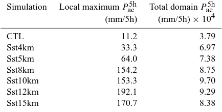
Simulation CTL shows weak and relatively disorganized banded structures with a spacing between them on the or-der of the minimum wavelength that can be represented by the model horizontal resolution (Fig. 2a), consistent with the inviscid linear model in the absence of small-scale terrain. Here, the small-scale disturbances required for convective triggering should be introduced either by physical mecha-nisms (e.g., adjustment of the initial profiles to the large-scale terrain), or nonphysical numerical errors. This is not a particularly relevant case for the atmosphere where small-scale roughness is always present at the surface, triggering lee waves that will play a dominant effect in embedded con-vection as discussed above. This fact becomes clear by com-parison of CTL with simulations that have small-scale ter-rain, the latter showing intense and well-organized convec-tive rain bands aligned parallel to the mean wind (Fig. 2b, c, d), with significant precipitation enhancement: total domain precipitation can be more than doubled and maximum local rainfall intensity can increase more than 17 times, depend-ing onlsst(Table 2). These results are qualitatively similar to Kirshbaum et al. (2007a) linear model predictions. However, for a single scale of terrain variability the analytical model

Table 1. Summary of WRF simulations population.

Simulation lsst (km) U (m s−1) Ts(K)

CTL – 10 285

Sst10km 10 10 285

Sst4km 4 10 285

Sst5km 5 10 285

Sst8km 8 10 285

Sst12km 12 10 285

Sst15km 15 10 285

Sst10km_T272.5 10 10 272.5

Sst10km_T275 10 10 275

Sst10km_T276 10 10 276

Sst10km_T277.5 10 10 277.5

Sst10km_T280 10 10 280

Sst10km_T282.5 10 10 282.5

Sst10km_T287.5 10 10 287.5

Sst10km_T290 10 10 290

Sst10km_T292.5 10 10 292.5

Sst10km_U5 10 5 285

Sst10km_U12.5 10 12.5 285

Sst10km_U15 10 15 285

Sst5km_T275 5 10 275

Sst5km_T277.5 5 10 277.5

Sst5km_T280 5 10 280

Sst5km_290 5 10 290

predicts a band spacing equal tolsstwhereas our simulations show banding withlsst/2 spacing. The reason is that while the linear model assumes that the upstream cloud edge posi-tion is fixed, the numerical simulaposi-tions show that bands can form at different x positions, generated by terrain features that are 90◦out of phase, a nonlinear effect not captured by the linear model.

M. Nogueira et al.: Toward subgrid-scale predictability 609

Fig. 2. Horizontal maps ofP_ac5h(black isolines at values 1, 10 and 50 mm/5h), and terrain height (gray scale, inm)for simulations (a) CTL, (b) Sst5km, (c) Sst10km and (d) Sst15km.

4 Empirical scaling analysis

4.1 The universal multifractal model

The existence of scale invariance in atmospheric fields is of-ten investigated by analyzing their statistical moments, which are expected to obey the generic multiscaling relation:

hϕq_λi =λK(q), (4)

where the angled brackets represent the statistical average,q is the moment order generalized to any positive real number, λ=L0

l is the scale ratio,L0being the outer scale of the cas-cade (the largest scale of variability) andl the scale of the observation, or simulation.ϕλ is a quantity that is on aver-age conserved from scale to scale in a similar way to what happens in turbulence cascade models. The turbulent flux is non-dimensionalized and normalized, such thathϕλi =1. In general geophysical fields are multifractals, i.e. the exponent Kis a nonlinear function ofq, and thus an infinity of expo-nents are required to characterize the scaling behavior. How-ever, one can use the UM framework to model the variation ofK withq for a conserved process, reducing the problem to two parameters (αandC1; Schertzer and Lovejoy, 1987):

K (q)=  

 C1

α−1(qα−q) , a6=1 C1qlog(q) , a=1

, (5)

The Levy index, α, defined in the interval [0,2], indicates the degree of multifractality (α=0 for monofractals); and the co-dimension of the mean singularity,C1, describes the sparseness or non-homogeneity of the mean of the process. The moment order must be positive (q >0)in this frame-work.

Table 2. Local maximum and domain total ofP_ac5hfield in simula-tions with different small-scale terrain wavelengths.

Simulation Local maximumP_ac5h Total domainP_ac5h (mm/5h) (mm/5h)×104

CTL 11.2 3.79

Sst4km 33.3 6.97

Sst5km 64.0 7.38

Sst8km 154.2 8.75

Sst10km 153.3 9.70

Sst12km 192.1 9.29

Sst15km 170.7 8.38

There is no physical basis to assume that a general ob-servable,f, (e.g., wind, temperature, rainfall, etc.) should be conserved on a scale by scale basis. In analogy with turbu-lence models, we may expect that observable fluctuations, 1f (l), over a distance,l, are related to a general turbulent conserved flux,ϕl, by

1f (l)=ϕη_llH. (6)

wind field,v)is not the direct result of a multiplicative cas-cade that role being reserved for the (cascas-cade conserved) energy flux,ε. The cascade conserved flux can have more complex forms that include nonlinear interactions of differ-ent fluxes, e.g., the Corsin–Obukhov law for passive scalar advection (Obukhov, 1949; Corsin, 1951):1ρ(l)=ξ1/3l1/3, whereξ =ϕl=χ3/2ε−1/2,χ being the scalar variance flux. In these classic turbulence cases, the laws relating the ob-servable fluctuations and conserved turbulent fluxes can be obtained from the governing dynamical equations, assuming isotropy, and via dimensional analysis. For rain and cloud processes (which generally cannot be assumed to behave as passive scalars), the values ofηandH are unknown, and so is the physical nature of the conserved flux. However it is still possible to perform scaling analysis. We start by taking the simplifying assumptionη=1, as usually done in similar previous works, noticing that if ϕλ is a pure multiplicative cascade then that is also true forϕη_λ, although with differ-ent C1values (e.g., Tessier et al., 1993; Stolle et al., 2009). The next step is to remove the influence of thelH term. One method used for this purpose is to rely on the absolute value of a finite difference gradient to compute the fluctuations at the highest resolution available,1f (lres)(see e.g., Lavallée et al., 1993; Tessier et al., 1993):

ϕ_λη=1f (lres)= n

f (x+lres, y)−f (x, y)2 (7) +f (x, y+lres)−f (x, y)2

o1/2 .

The flux estimates given by Eq. (7) are systematically de-graded to lower resolutions (lower values ofλ)by spatial av-eraging. The Double Trace Moment (DTM) technique (e.g., Lavallée et al., 1993) can be used subsequently to estimate αandC1. Notice that the values of the UM parameters esti-mated from data generated by numerical models are not the same as the ones obtained from observations due to cascade cutoff by model resolution and model domain, but it is pos-sible to convert between them (Stolle et al., 2009). Never-theless, incorrect representation of physical processes in the models cannot be corrected. In the present work we aim only to investigate the variation of the UM parameters in numer-ical simulations with similar setup, so no conversion is re-quired.

Spectral analysis can also be used to investigate the be-havior of a field over a wide range of scales. The spatial Fourier power spectrum,E(kx, ky), is computed by multi-plying the 2-D fast Fourier transform of a field by its com-plex conjugate, wherekxandkyare the wavenumber compo-nents. The power spectrum is then averaged angularly about kx, ky=(0,0) to yield what is usually called isotropic power spectrum E(k), with k=qk2

x+k2y. Spatial scaling invariance manifests itself as log–log linearity of the power spectrum in space:

E(k)∼k−β−1, (8)

whereβ is the spectral exponent and the addition of−1 in the exponent is required due radial averaging is phase space (e.g., Turcotte, 1992; Lovejoy et al., 2008b). Least square regression is used to estimateβ from a log–log plot ofE(k) againstk.

The spectral exponent is related to the UM parameters by (Tessier et al., 1993)

β=1+2H−K(2). (9)

Finally, we estimateH from the slope of the log–log plot of the first order structure function against the lag, as de-scribed by Harris et al. (2001), Nykanen (2008) and Lovejoy et al. (2008a, b).

4.2 Scaling in simulated 2-D fields

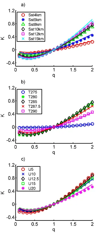
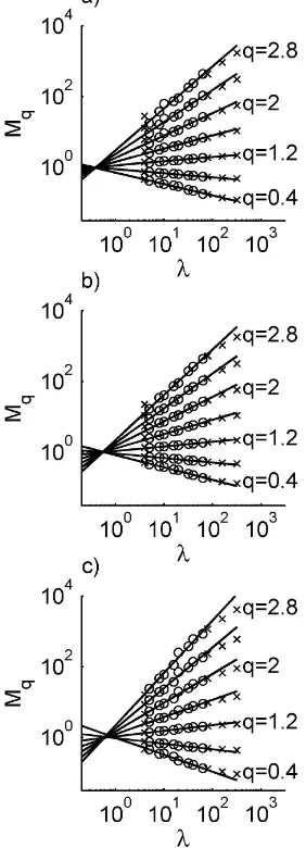
The empirical scaling analysis described above is applied to surface accumulated precipitation spatial fields over 5 h sim-ulations,P_ac5h. Here the constant value 80 km (scaling analy-sis domain length) was used for the cascade outer scale,L0. Changing the chosen value of L0 has no effect on the es-timated value of the slope of the fitted lines, i.e., on K(q) and respective UM parameter estimation. Figure 3a–c show log–log plots of Mq against λfor Pac5h fields for three dif-ferent simulations. The lines are only fitted to the range of scales that are well resolved by the model, i.e., larger than 51x(=1.25 km) and smaller than aboutL0/4(=20 km). For q≤2 the linear fits are good implying that statistical scale invariance predicted by Eq. (4) is a good representation, and that there are no characteristic scales or scale breaks for the considered ranges ofq andλ (from∼1 to ∼20 km). This range ofq is similar to the ones found in literature for sim-ilar analysis (e.g Douglas and Barros, 2003; Lovejoy et al., 2008a, b; Nykanen, 2008; de Lima and de Lima, 2009). Some simulations show persistent deviations from linear behavior at particular scales, but the relation between these scales and lsst varies between simulations, suggesting that the small-scale terrain wavelength is not (statistically) a characteristic scale in the rain fields. The same spatial scaling analysis was repeated for theP_ac5h fields resulting from all simulations in Table 1, all of them showing the same robust scaling behavior (linear relations).

M. Nogueira et al.: Toward subgrid-scale predictability 611

Fig. 3. Relationship betweenMqandλfor different values ofq.Mq is computed fromP_ac5hfrom simulation (a) Sst5km, (b) Sst10km, (c) Sst15km. The scales considered on the analysis are marked by “o” while “x” marks the ones not considered. The plots are on a log–log scale.

which display a complex nonlinear variation with simula-tion attributes. A particularly remarkable feature is the abrupt transition in both UM parameters forTsbetween 275 K and 285 K. The transition has a physical correspondence when interpreted against the spatial rainfall patterns (red lines in Fig. 6), capturing the evolution from terrain-following (more stratiform) and less intense rainfall fields in the colder sim-ulation cases to well-organized and intense bands for simu-lations at intermediate temperatures. For warmer simusimu-lations the rainfall pattern changes again to more intense but less or-ganized (more cellular) convective features (Fig. 6d), and the UM parameters also show variation (Fig. 5c and d). These differences in convective dynamics have important effects in

Fig. 4. The scaling exponent function,K(q)for (a) varyinglsst, (b) varyingTs withlsst=10 km and (c) varyingU withlsst=10 km. The empirical estimatedK(q)is showed with markers and the UM model fit is represented by full line.

rainfall intensities and patterns leading to high localized rain-fall accumulation values (Table 3, and see also Kirhsbaum and Durran, 2005b and Fuhrer and Schär, 2007).

Table 3. Local maximum ofP_ac5h,qcandqi fields and domain totalPac5hfor simulations with different temperature profiles.

Simulation Local maximum of Total domain Local maximum of Local maximum of P_ac5h(mm/5h) P_ac5h(mm/5h)×104 qc(g kg−1) qi(g kg−1)

Sst10km_T272.5_WR 0.00 0.00 0.53 –

Sst10km_T272.5 1.90 4.79 0.24 0.11

Sst10km_T275 1.75 3.63 0.27 0.13

Sst10km_T276 1.80 3.05 0.33 0.13

Sst10km_T277.5 0.33 0.07 0.71 0.00

Sst10km_T280 23.77 1.20 1.10 0.00

Sst10km_T282.5 83.72 2.83 1.34 0.00

Sst10km 153.28 4.68 1.49 0.00

Sst10km_T287.5 143.06 9.20 1.57 0.83

Sst10km_T290 214.45 31.59 1.79 2.13

Sst10km_T292.5 258.87 76.43 2.18 5.25

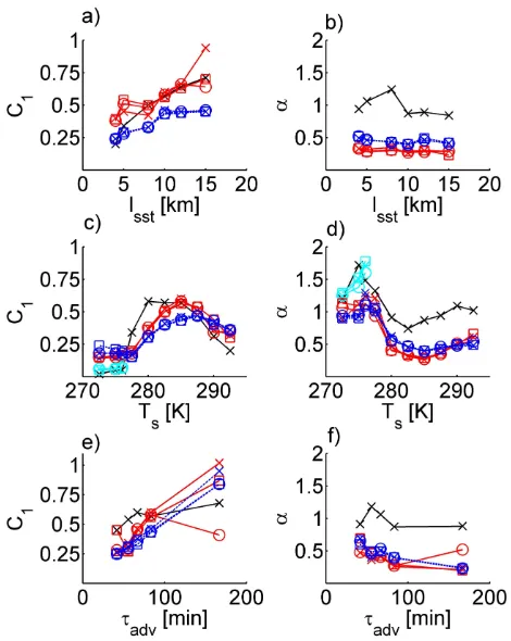
Fig. 5. Relationship between UM parameters (C1andα)and: (a, b) lsst; (c, d)Ts; and (e, f)τadv. Black lines represent values computed fromP_ac5h, red and blue lines are computed fromqcatzqcmaxand z=1100 m, respectively. Light blue markers are computed from ice mixing ratio fields at the level of their maximum intensity. “x”, “o”, “” markers represent simulation times 05:00 h, 04:00 h and 03:00 h, respectively.

and blue at z=1100 m in Fig. 5). In particular the transi-tion between colder and warmer cases is again clear. Both αandC1show similar values at the different times, due to the quasi-stationary state of the convective structures that is

Fig. 6. Horizontal cross sections ofPac5h (red isolines),qc fields at zq_cmax at 04:00 h (black isolines) and qi at the level of its maximum intensity at 04:00 h (blue isolines) from simulations (a) Sst10km_T272.5, (b) Sst10km_T277.5, (c) Sst10km and (d) Sst10km_T290. Grayscale represents topographic elevation (in me-ters).

M. Nogueira et al.: Toward subgrid-scale predictability 613

Fig. 7. Relationship betweenMqandλfor different values ofq.Mq is computed fromqcatzqcmaxat 04:00 h for simulation (a) Sst5km, (b) Sst10km and (c) Sst15km. The scales considered on the analysis are marked by “o” while “x” marks the ones not considered. The plots are on a log–log scale.

for Sst15km at 05:00 h computed fromqcatzqcmaxis quite different from the one at 04:00 h, which is easily understood by examining Fig. 8: in Sst10km thezq_cmaxlevel crosses the core of the cloud band, the same happening for Sst15km at 04:00 h, while at Sst15km at 05:00 h it is actually crossing a region of instabilities that has formed on the top region of the band, resulting in a different horizontal pattern and asso-ciated scaling parameters. The large variation inC1 for the largest advective timescaleτadvat different times has a simi-lar explanation.

The cumulative rainfall field analyzed here is viewed as representative of the entire simulated convective rain event. It is important to stress that a time integrated quantity will depend on the evolution of the system during the

integra-Fig. 8. Cross sections (xz) ofqcat theyposition of its maximum intensity for simulations (a) Sst10km at 04:00 h, (b) Sst15km at 04:00 h and (c) Sst15km at 05:00 h. The solid black line represents topography. The upper and lower black dashed lines represent the levelszq_cmaxandz=1100 m, respectively.

tion interval and the specific quantitative values of scaling parameters should change during this period due to the tran-sient nature of the interactions among various physical pro-cesses. Presently, at this stage of the research, the analysis is focused on the spatial properties of the accumulated pre-cipitation fields for a specific time of integration in a manner consistent with standard rainfall observations that consist of rainfall accumulations over a measurement timescale. Down-scaling is critical to obtain robust spatial distributions of rain-fall for use in hydrological studies and applications.

4.3 Scaling in cloud simulated fields – 3-D analysis

Fig. 9. Relationship betweenMq andλfor different values ofq. Mqis computed fromqcat 04:00 h for simulations (a) Sst5km, (b) Sst10km, (c) Sst15km. The scales considered on the analysis are marked by “o” while “x” marks the ones not considered. The plots are on log–log scale.

absence of characteristic scales. The presence of scaling be-havior for the entire volume implies that concurrent spatial structures (e.g., band core region, instabilities at the top of the bands, clouds that form downstream of the large scale orography, among others, Fig. 8) fall in the same average horizontal scaling regime. The scaling behavior in the ver-tical direction is not investigated here due to data limitations associated with the limited number of vertical levels in the model (see Sect. 2) together with the fact that we are looking at instantaneous realizations of fields rather than ensemble average statistics. But in other cases it could be investigated using a different set of UM parameters to describe anisotropy

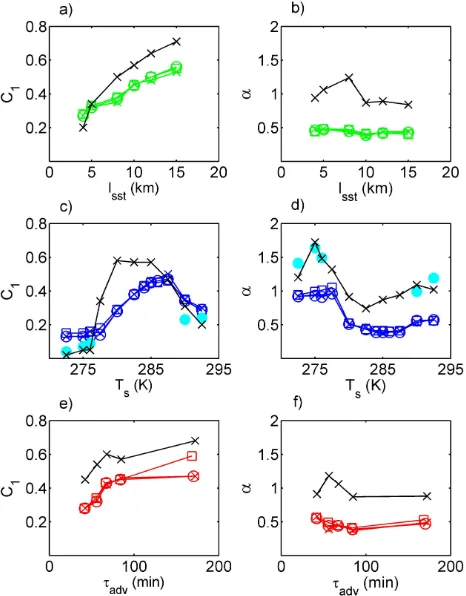
Fig. 10.C1and αcomputed from 3-D averages ofqc horizontal fluctuations against: (a, b)lsst, (c, d)Tsand (e, f)τadv. Black lines represent values computed fromP_ac5h. Green, blue and red lines are computed fromqc. The light blue markers lines are computed from qi. “x”, “o” and “” markers represent simulation times 05:00 h, 04:00 h and 03:00 h, respectively.

between horizontal and vertical directions (see e.g., Lovejoy et al., 1987; Lazarev et al., 1994; Radkevich et al., 2007).

M. Nogueira et al.: Toward subgrid-scale predictability 615

Fig. 11.C1andαcomputed from 3-D averages ofqc horizontal fluctuations against: (a, b)N_m2; (c, d) cf×N_m2; and (e, f) CAPE. Blue lines and markers are computed from simulations with vary-ingTsandlsst=10 km, pink from simulations with varyingTsand lsst=5 km, red for varyingτadvand green for varyinglsst. Plots (g, h) showC1andαagainst cf×Nm2 for all simulations. Black mark-ers in plots (b) and (h) represent simulation Sst10km (i.e., the base case). “x”, “o” and “” markers represent simulation times 05:00 h, 04:00 h and 03:00 h, respectively.

question as to the character of the underlying physics and of this flow transition for highly unstable flows, not unlike the transition to high Reynolds numbers in the case of fully de-veloped turbulence turbulence. The fields with the strongest instability values are not necessarily the warmer ones as de-fined by the initial conditions, as the averageN_m2value can be

significantly altered by the release of latent heating or due to the presence of downstream stable clouds and other features. To capture the effect of space–time co-localization of moist instability release and moist processes,N_m2can be mul-tiplied by a measure of the cloud fraction, cf, defined here by the ratio of number of grid points that exceed the chosen qc threshold to the total number of points. This transforma-tion gives a measure of the overall realized moist instabil-ity at a given point in time, and provides a physically based framework to arrange the simulations in the order of colder (more stable, higher cf×Nm2)to warmer profiles (more un-stable, lower cf×Nm2), consequently yielding more robust relationships (Fig. 11c and d). Indeed, this result holds for different values of the threshold, and the transition between stable and unstable cases becomes clearer in these plots. The stable region shows nearly constant UM parameters, with lower values ofC1associated with a more space filling mean component in stratiform clouds as compared to more local-ized convective structures; the region of low reallocal-ized instabil-ity corresponds to simulations that produce quasi-stationary rainbands, in agreement with the numerical experiments of Kirshbaum and Durran (2005a) who found that marginal po-tential instability and moderate wind speeds were the most favorable atmospheric conditions for convective bands to de-velop. This region displays complex variation of the scal-ing parameters that might be associated with the presence of different regimes due to competition between buoyancy and mechanical generation/dissipation of turbulence. Further in-vestigation – with a larger population of simulations in this specific region of instability values – is necessary for further confirmation of this finding. In particular, the role of wind shear (usually understood as a mechanical turbulence gener-ator) in band generation is not clear and requires more de-tailed analysis. The bands form in the absence of any basic-state vertical shear (as it is seen in our simulation and also in Kirshbaum and Durran, 2005a; and Kirhsbaum et al., 2007b), although wind shear will dynamically develop in these sim-ulations eventually due, for example, to adjustment to terrain or formation of localized convective circulations. Kirshbaum and Durran (2005a) also found that in some cases, wind shear can actually suppress rainbands. Figure 11c and d also sug-gest that for higher instability conditions, when free convec-tion dominates, and corresponding to the more cellular and disorganized patterns, the parameter variation becomes less complex.

markers), particularly in the region of low instability (sta-ble cases). Also the pink curves in Fig. 11c, d, and g and 11h show that, for the same initial temperature profiles but lsst=5 km instead of 10 km, different values ofC1 are ob-tained. Thus cf×Nm2alone cannot be used as a single pre-dictor for both UM parameters, and variation withlsst and τadvhas to be considered separately.

As mentioned earlier, Perica and Foufoula-Georgiou (1996) found a linear dependency of statistical scaling pa-rameters on another atmospheric stability measure, the Con-vective Available Potential Energy (CAPE), for a small num-ber of rainfall fields of selected convective storms over rel-atively flat topography. This result was tested in our simu-lated fields which have a wider range of CAPE values, and a more complex nonlinear relation was obtained (Fig. 11e and f). Compared toN_m2, the use of CAPE has the disadvantage that the stable range of the profiles is ambiguous (CAPE=0 for all stable cases), which presents a problem unless UM parameters were shown to be constant for all stable cases. Nevertheless, note that the unstable/stable transition of the parameters is still clear as CAPE goes to zero, as well as the complex nonlinear behavior for the small magnitude insta-bility values – the banded cases – and again less complex behavior for higher magnitude instability values – cellular disorganized cases. This is consistent with Kirshbaum and Durran (2005b) who proposed that the distinction between more banded and cellular cases is related to enhanced suscep-tibility to free convection, with larger CAPE implying more cellular structures. They suggest that Convective INhibtion (CIN) could be an important parameter as well, but all our simulations have very small values of CIN and are not suit-able for such analysis.

4.4 Relations between different scaling fields

In both 2- and 3-D analysis, UM parameters computed from P_ac5h andqc show clear relations for certain ranges of simu-lation properties, either in the shape of the variation curve in Fig. 5a, c, d and Fig. 10a, c, d, e, or for the exact values of the parameter, as can be seen for example in Fig. 5a forC1 computed fromqcatzqcmaxforlsst≥8 km and C1computed fromz=1100 m for smallerlsst(also in Fig. 5c, see theC1 computed fromqcatzqcmaxforTs≥285 K, and in Fig. 11c for Ts≥287.5 K). For the 2-D analysis these relationships depend on the chosen vertical level, sometimes best relating to the level of maximum intensity, sometimes to some other level, which makes its use difficult in practical applications, further supporting the 3-D analysis.

Figures 5c, d and 10c, d show that for colder simula-tions (Ts≤277.5 K) both UM parameters computed from P_ac5h are very similar to the ones computed from ice phase (snow+ice+graupel) mixing ratio fields,qi, which is par-ticularly remarkable in the 3-D analysis. The role of cold mi-crophysics on precipitation processes is also clear in simula-tion Sst10km_T272.5_WR (which is exactly the same as in

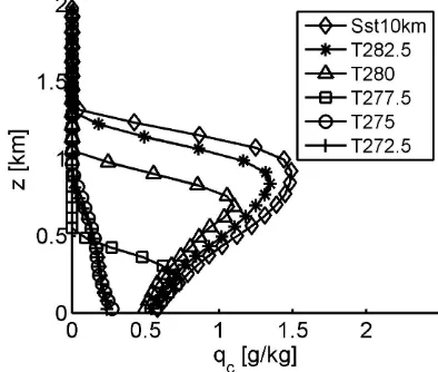
Sst10km_T272.5, except that the Kessler warm rain scheme is used in WRF and ice microphysics is turned off). The simulation with warm rain processes only produces a cloud pattern similar to the one including cold microphysics, but it yields zero P_ac5h (Table 3). This result is strengthened by the fact that below 277.5 K the values of precipitation inten-sity andqi increase with decreasing temperature (Table 3). Finally, it is also apparent in Fig. 6a that for the colder case there is a clear relation between theP_ac5h(red line) and qi (blue line) patterns, while theqc (black line) seems to be more closely related to the underlying topography (grey scale). If the temperature is slightly raised, bothqi andPac5h go to zero (Fig. 6b and Table 3). If the temperature is raised further, well-organized cloud bands form with a clearly asso-ciatedP_ac5hpattern and no ice phase (Fig. 6c). Besides varying N_m2, changingTsalso changes the amounts of water in each phase and the vertical structure of the clouds, particularly the cloud depth (Fig. 12), which the linear theory also predicts as being an important parameter in embedded convection. For the warmer cases considered here, the cloud depth growths enough so that ice processes become important again (blue lines in Fig. 6d and Table 3), but the precipitation pattern now seems to be more related to qc (Fig. 6d). In these warmer cases, the parameterC1 fromPac5h seems to relate better to qc while αseems to relate better toqi (Fig. 10c, d). Over-all, these results suggest that scaling of the simulated total precipitation fields is a complex function of the scaling of several other fields including water mixing ratio in the differ-ent phases, and probably also small-scale terrain spectra and τadv. That is, the scaling of the integral precipitation fields reflects the underlying governing physical processes, which change with time and space as weather systems evolve and propagate over complex terrain.

4.5 Spectral analysis

M. Nogueira et al.: Toward subgrid-scale predictability 617

Fig. 12. Vertical profiles ofqc at the position of their maximum intensity at 04:00 h, for simulations withlsst=10 km and varying Ts.

boundary of the range was reduced to a valueL0/8. Outside this range, we do not have enough information on the power spectrum of the field.

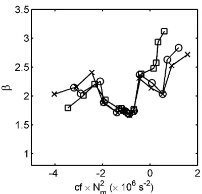
The black dashed lines in Fig. 13 are least-square fits to the considered range of scales (wavenumbers) of the power spectrum. There is a clear mean linear trend (scaling) in the log–log power spectra, withR2 values for the least-square fits always above 0.90. Peaks in the power spectra, particu-larly evident in the intermediate banded case spectrum (mid-dle spectra in Fig. 13), are consistent with harmonics re-sulting from the banded pattern. This behavior is expected when analyzing single realizations of cloud fields (e.g., Har-ris et al., 2001), and more so for events over complex ter-rain when orographic forcing is dominant (e.g., see scaling analysis in Barros et al., 2004). The scaling analysis was repeated here for all the simulations withlsst=10 km and varyingTs, all of them showing a mean linear trend in the log–log power spectra. Figure 14 shows that the variation of fitted values ofβwith cf×N_m2 displays similar transitions to the ones found for UM parameters, between stable/unstable cases and banded/disorganized convection. The location of the stable/unstable transition now seems to have been shifted to values slightly lower thanN_m2=0. For numerical model-ing parameterizations or downscalmodel-ing, the exact location of this transition should be determined using a large data base of realistic simulations. Yet, the existence of such transition alone, which is supported by both spectra and moment scal-ing analysis and agrees with expected physical behavior such as for example the Richardson number criteria in boundary layer stability analysis, is an important finding in itself. The colder stratiform cases show some spread inβ values that was not found in the UM parameters, including an unphys-icalβ >3 value. It should be taken into consideration these cases have shallower clouds (Fig. 12), which imply fewer

Fig. 13. Log–log plots of isotropic power spectra computed from horizontalqcfield at 04:00 h averaged over several vertical levels, from simulations: Sst10km_T292.5 (top), Sst10km (middle) and Sst10km_T272.5 (bottom). Only the range of scales between 51x and aboutL0/8 is represented. The black dashed lines are least square fits to the spectra.

levels of data for computation, along with low intensities of cloud fields, making them susceptible to computational un-certainty in the spectral exponent, adding to the limitations in the spectral analysis. The highly idealized topography with a superposed 2-D sinusoidal field used in the simulations here was designed to replicate and build upon previous works that used linear theory to investigate the development of oro-graphic convection, and is not scaling. The structure of strat-iform (terrain following) and orographically triggered con-vective fields is very influenced by the properties of the topo-graphic elevation (e.g., Barros and Lettenmaier, 1994; Kirsh-baum and Durran, 2004; Barros et al., 2004), and therefore a linkage between their scaling properties should exist. Follow up work, with realistic terrain should give further insight into this question.

Fig. 14. Relationship betweenβ(computed from horizontalqcfield averaged over several vertical levels) and cf×N_m2(×10−5s−2). “x”, “o”, “” markers represent simulation times 05:00 h, 04:00 h and 03:00 h, respectively.

5 Summary and discussion

Linear stability analysis reveals that embedded convective structures are the result of unstable growth of small-scale dis-turbances, which should be very important in determining the predictability of orographic precipitation. They also suggest the governing role of parameters such as atmospheric stabil-ity, advective timescale, small-scale terrain spectra and cloud depth. The results from idealized numerical simulations of orographic convective precipitation qualitatively agree with these predictions. Particularly, they show that the represen-tation of small-scale terrain (and associated lee waves) plays a very important role for these events, controlling the band spacing and significantly enhancing the convective intensity and rainfall amounts. But these simple models are unable to do any quantitative predictions or even predict the correct pattern (except in very particular cases) due to the presence of nonlinear effects, and alternative nonlinear models are re-quired.

As pointed out by Schertzer and Lovejoy (1992), the con-tributions of small-scale activity to much larger scales are non-negligible, and indeed the corresponding variability has the most extreme behavior which explains in part the rea-son why multifractals have been successful on the study of extreme events. In fact several previous works reported sta-tistical multiscaling behavior to be a very general property of geophysical fields (including rain and clouds), provid-ing a convenient alternative framework due to its theoreti-cal simplicity, its ability to handle nonlinear dynamics over very wide range of scales, its potential for downscaling ap-plications and the fact that the convective events studied here are a particular kind of turbulent flow and hence a

statisti-cal approach to the problem is appropriate. This multisstatisti-caling behavior holds for statistical moments and isotropic power spectra of the simulated rain and cloud fields in the consid-ered range of scales (∼1 km to∼20 km). The universal mul-tifractal model reproduces quite well the empirical estimates of the horizontal scaling exponent function,K(q), and can be used to quantify the multiscaling behavior of the fields. Analysis of single horizontal sections of cloud fields revealed variation of the scaling parameters with vertical position. We argue that if we use an average over several horizontal sec-tions at different vertical levels, we obtain estimates for the horizontal parameters of the entire volume, while the vertical structure should be represented by a different set of (vertical) scaling parameters. This transient 3-D anisotropic scaling framework seems to be a promising starting point to investi-gate relations between the statistical and physical properties and perform downscaling for mesoscale events. Results from both 2- and 3-D approaches revealed significant variations ofK(q)and respective UM parameters with small-scale ter-rain spectra, atmospheric stability and advective timescale. Therefore, the representation of sub-grid scale variability of cloud and rainfall fields using statistical multifractal diagnos-tics would intrinsically depend not only on the properties of the field itself, but also on particular geographic location and atmospheric conditions, bringing the necessity of developing relationships to predict the scaling parameters from coarse grid atmospheric data and terrain spectra. However, the re-sults also suggest that the development of such relationships is far from being trivial because they appear to involve com-plex nonlinear behavior.

A particularly robust behavior found here is the abrupt transition in the UM parameters between stable and unstable cases, which has a clear physical correspondence as a tran-sition from a more stratiform to a more organized (banded) convective regime. This behavior is also found in the spectral exponentβ. Another instability measure, CAPE, also seems to be a good predictor, but it is unable to distinguish between the different stable cases and CIN might have to be used in conjunction.N_m2also has the advantage of allowing a linkage with the analytical models where it appears explicitly, which is not so clear for CAPE. It was also found that the scaling of the surface accumulated precipitation field (usually an impor-tant field to be parameterized and downscaled) is a complex function of the horizontal scaling of several other fields such as water mixing ratios in the different phases and probably lsstandτadv.

M. Nogueira et al.: Toward subgrid-scale predictability 619

dependency of the scaling parameters is introduced by the temporal evolution of the atmospheric conditions, and the usually small time step used in numerical simulations can be advantageous to achieve a high temporal representation. Further improvements could include scaling constraints us-ing higher-order moments.

Finally, it is important to point out some limitations of our study. In order to investigate the dependence of the mul-tifractal properties on mean properties, a limited range of highly idealized simulations are used where we can control the mean atmosphere with a small number of simulation pa-rameters. Because our work suggests a transient dependence of the scaling on mean properties, the analysis is performed on instantaneous fields, rather than ensemble averages, which increases the volume of data necessary for analysis. Horizon-tal isotropy is assumed, and it is important to stress that the issue of existence of horizontal anisotropy must be tackled in the future. The solutions show robust horizontal scaling even though the only external forcing is a very simple terrain with poor scaling and the initial conditions are horizontally homo-geneous. In realistic cases, the atmosphere and terrain forcing will themselves be scaling, which might influence the scaling of the solutions. Models such as WRF involve many subgrid scale parameterizations which vary among model configura-tions. Here we use parameterizations only for subgrid tur-bulence closure and microphysical processes. Whether these parameterizations introduce unphysical scaling behavior in the models at resolved scales, and whether the scaling de-pends on the particular chosen parameterizations are legit-imate questions. Furthermore, in the real atmosphere there are many other effects not considered here such as radia-tion, earth rotaradia-tion, surface and boundary layer effects which might introduce further complications and influence the scal-ing. In this study, however we spell out unambiguously what processes are resolved or not, and there is general a body of literature that shows that the resolution adopted can re-solve explicitly dominant convective structures (see for ex-ample Fuhrer and Schär, 2007). In fact, as pointed out in Sect. 2, our simulations are based on previous work where the authors showed that they reproduce the essential features of the observed convective structures in the Oregon Coastal Range. Harris et al. (2001) compared the scaling observed and model produced precipitation fields at 3-km resolution, finding an encouragingly similar behavior at scales above 5 times the resolution (i.e., 15 km). Although they simulated realistic cases with different model and parameterizations than here, the model is based on the same governing equa-tions. Our assumption here is that our simulations, based on nonlinear, compressible and non-hydrostatic Navier–Stokes equations coupled with the thermodynamics equations in the WRF model under the specified forcing conditions represent the key physical processes of interest and that the multifrac-tal parameters can be used to describe the behavior of the simulated system in the explicitly well-resolved scales. It is important to stress that the fields resulting from numerical

simulations should reproduce the scaling in geophysical ob-servations if they are to be realistic. Furthermore, we apply multifractal analysis not as means to find universal parame-ters that will exhibit consistency, though that could be a re-sult, but rather as a mathematical model can capture, at any given scale, variability that reflects a large dynamical range of the phenomena determined by the long-range dependen-cies. Thus, what is consistent is the model used to describe variability; we then make use of the multifractal model pa-rameters as metrics that can help interpret model dynamics and thermodynamics in a systematic way. The presence of an underlying multifractal behavior is robustly supported by the evidence presented: a clear mean linear trend in the spec-tral analysis in conjunction with the robust scaling in the mo-ment analysis, which is less sensitive to the data limitations and reveals robust scaling behavior up to orders of about 2, as it is typically found in atmospheric fields and reported in literature consistent with the scope of the present manuscript. Although much insight was gained into scaling depen-dencies, particularly the presence of transient dependence of scaling parameters on mean conditions found here, an inves-tigation on observational atmospheric data and realistic nu-merical simulations is warranted, along with further support to whether numerical weather prediction models are able to reproduce, at least to some extent, the multifractal proper-ties of simulated fields and what is the effect of the particular parameterizations chosen on the scaling. This is currently on-going work.

Acknowledgements. The authors would like to thank three anonymous referees for their comments and suggestions which helped to significantly improve the manuscript. This research is supported by the Portuguese Foundation for Science and Technology (FCT) under grants SFRH/BD/61148/2009 and PTDC/CTE-ATM/119922/2010, and NASA grant NN1010H66G and NSF grant EAR-0711430 with the second author.

Edited by: I. Tchiguirinskaia

Reviewed by: A. A. Carsteanu and three anonymous referees

References

Barros, A. P. and Lettenmaier, D. P.: Dynamic modeling of oro-graphically induced precipitation, Rev. Geophys., 32, 265–284, 1994.

Barros, A. P., Kim, G., Williams, E., and Nesbitt, S. W.: Probing orographic controls in the Himalayas during the monsoon us-ing satellite imagery, Nat. Hazards Earth Syst. Sci., 4, 29–51, doi:10.5194/nhess-4-29-2004, 2004.

Bindlish, R. and Barros., A. P.: Aggregation of digital terrain data using a modified fractal interpolation scheme, Comput. Geosci. (UK), 22, 907–917, 1996.

Cosma, S., Richard, E., and Miniscloux, F.: The role of small-scale orographic features in the spatial distribution of precipitation, Q. J. Roy. Meteor. Soc., 128, 75–92, 2002.

Deidda, R: Rainfall downscaling in a space-time multifractal frame-work, Water Resour. Res., 36, 1779–1794, 2000.

Deidda, R., Badas, M. G., and Piga, E.: Space-time scaling in high-intensity Tropical Ocean Global Atmosphere Coupled Ocean-Atmosphere Response Experiment (TOGA-COARE) storms, Water Resour. Res., 40, W02506, doi:10.1029/2003WR002574, 2004.

de Lima, M. I. P. and de Lima, J. L. M. P.: Investigating the multi-fractality of point precipitation in the Madeira archipelago, Non-lin. Processes Geophys., 16, 299–311, doi:10.5194/npg-16-299-2009, 2009.

Douglas E. M. and Barros, A. P.: Probable Maximum Precipita-tion EstimaPrecipita-tion Using Multifractals: ApplicaPrecipita-tion in the Eastern United State, J. Hydrometeor., 4, 1012–1024, 2003.

Emanuel, K.-A.: Atmospheric Convection, Oxford University Press, New York, 1994.

Fuhrer, O. and Schär, C.: Embedded cellular convection in moist flow past topography, J. Atmos. Sci., 62, 2810–2828, 2005. Fuhrer, O. and Schär, C.: Dynamics of Orographically Triggered

Banded Convection in Sheared Moist Orographic Flows, J. At-mos. Sci, 64, 3542–3561, 2007.

Gupta, V. K. and Waymire, E. C.: A statistical analysis of mesoscale rainfall as a random cascade, J. Appl. Meteor., 32, 251–267, 1993.

Harris, D., Foufoula-Georgiou, E., Droegemeier K. K., and Levit, J. J: Multiscale Properties of a High-Resolution Precipitation Fore-cast, J. Hydrometeor., 2, 406–418, 2001.

Kirshbaum, D. J. and Durran, D. R.: Factors governing cellular con-vection in orographic precipitation, J. Atmos. Sci., 61, 682–698, 2004.

Kirshbaum, D. J. and Durran, D. R.: Atmospheric factors governing banded orographic convection, J. Atmos. Sci., 62, 3758–3774, 2005a.

Kirshbaum, D. J. and Durran, D. R.: Observations and modeling of banded orographic convection, J. Atmos. Sci., 62, 1463–1479, 2005b.

Kirshbaum, D. J., Rotunno, R., and Bryan, G. H.: The Spacing of Orographic Rainbands Triggered by Small-Scale Topography, J. Atmos. Sci., 64, 1530–1549, 2007a.

Kirshbaum, D. J., Bryan, G. H., Rotunno, R., and Durran, D. R.: The triggering of orographic rainbands by small-scale topography, J. Atmos. Sci„ 66, 1530–1549, 2007b.

Kolmogorov, A. N.: Local structure of turbulence in an incompress-ible liquid for very large Reynolds numbers, Proc. Acad. Sci. USSR. Geochem Sect., 30, 299–303, 1941.

Kuo, H. L.: Perturbations of plane Couette flow in stratified fluid and origin of cloud streets, Phys. Fluids, 6, 195–211, 1963. Lavallée, D., Lovejoy, S., Schertzer, D., and Ladoy, P.: Nonlinear

variability and Landscape topography: analysis and simulation, Fractals in Geography, edited by: De Cola, L. and Lam, N., 158– 192, PTR, Prentice Hall, 1993.

Lazarev, A., Schertzer, D., Lovejoy, S., and Chigirinskaya, Y.: Uni-fied multifractal atmospheric dynamics tested in the tropics: part II, vertical scaling and generalized scale invariance, Nonlin. Processes Geophys., 1, 115–123, doi:10.5194/npg-1-115-1994, 1994.

Lovejoy, S., Schertzer, D., and Tsonis, A. A.: Functional box-counting and multiple elliptical dimensions in rain, Science, 235, 1036–1038, 1987.

Lovejoy, S., Schertzer, D., and Allaire, V.: The remarkable wide range spatial scaling of TRMM precipitation, Atmos. Res., 90, 10–32, 2008a.

Lovejoy, S., Tarquis, A. M., Gaonac’h, H., and Schertzer, D.: Single- and Multiscale Remote Sensing Techniques, Multifrac-tals, and MODIS Derived Vegetation and Soil Moisture, Vadose Zone Journal, 7, 533–546, 2008b.

Miniscloux, F., Creutin, J. D., and Anquetin, S.: Geostatistical anal-ysis of orographic rain-bands, J. Appl. Meteor., 40, 1835–1854, 2001.

Nykanen, D. K.: Linkages between Orographic Forcing and the Scaling Properties of Convective Rainfall in Mountainous Re-gions, J. Hydrometeor., 9, 327–347, 2008.

Over, T. M. and Gupta, V. K.: Statistical analysis of mesoscale rain-fall: Dependence of a random cascade generator on large-scale forcing, J. Appl. Meteor., 33, 1526–1542, 1994.

Obukhov, A., Structure of the Temperature Field in a Turbulent Flow, lzv. Akad. Nauk. SSSR Set. Geogr.l Jeofiz, 13, 55–69, 1949.

Perica, S. and Foufoula-Georgiou, E.: Linkage of scaling and ther-modynamic parameters of rainfall: Results from midlatitude mesoscale convective systems, J. Geophys. Res., 101, 7431– 7448, 1996.

Radkevich, A., Lovejoy, S., Strawbridge, K., and Schertzer, D.: The elliptical dimension of space-time atmospheric stratification of passive admixtures using lidar data, Physica A, 382, 597–615, 2007.

Rebora, N., Ferraris, L., von Hardenber, J., and Provenzale, A.: RainFARM: Rainfall Downscaling by a Filtered Autoregressive Model, J. Hydrometeor., 7, 724–738, 2006.

Schertzer, D. and Lovejoy, S.: Physical modeling and analysis of rain and clouds by anisotropic and clouds by anisotropic scal-ing of multiplicative processes, J. Geophys. Res., 92, 9692–9714, 1987.

Schertzer, D. and Lovejoy, S.: Hard and Soft Multifractal pro-cesses, Physica A, 185, 187–194, 1992.

Skamarock, W. C., Klemp, J. B., Dudhia, J., Gill, D. O., Barker, D. M., Wang, W., and Powers, J. G.: A description of the ad-vanced research WRF Version 3, NCAR Tech. Note, NCAR/TN-475+STR, 113 pp., 2008

Stolle, J., Lovejoy, S., and Schertzer, D.: The stochastic multi-plicative cascade structure of deterministic numerical models of the atmosphere, Nonlin. Processes Geophys., 16, 607–621, doi:10.5194/npg-16-607-2009, 2009.

Tessier, Y., Lovejoy, S., and Schertzer, D.: Universal multifractals: Theory and observations for rain and clouds, J. Appl. Meteor., 32, 223–250, 1993.

Turcotte, D. L: Fractals and chaos in geology and geophysics: Cam-bridge University Press, New York, 221 pp., 1992.