Why could ice ages be unpredictable?

www.clim-past.net/9/2253/2013/ doi:10.5194/cp-9-2253-2013

© Author(s) 2013. CC Attribution 3.0 License.

Climate

of the Past

Why could ice ages be unpredictable?

M. Crucifix

Earth and Life Institute, Georges Lemaître Centre for Earth and Climate Research Université catholique de Louvain, Louvain-la-Neuve, Belgium

Correspondence to: M. Crucifix ([email protected])

Received: 4 February 2013 – Published in Clim. Past Discuss.: 20 February 2013 Revised: 30 June 2013 – Accepted: 28 August 2013 – Published: 9 October 2013

Abstract. It is commonly accepted that the variations of Earth’s orbit and obliquity control the timing of Pleistocene glacial–interglacial cycles. Evidence comes from power spectrum analysis of palaeoclimate records and from inspec-tion of the timing of glacial and deglacial transiinspec-tions. How-ever, we do not know how tight this control is. Is it, for ex-ample, conceivable that random climatic fluctuations could cause a delay in deglaciation, bad enough to skip a full pre-cession or obliquity cycle and subsequently modify the se-quence of ice ages?

To address this question, seven previously published con-ceptual models of ice ages are analysed by reference to the notion of generalised synchronisation. Insight is being gained by comparing the effects of the astronomical forcing with idealised forcings composed of only one or two peri-odic components. In general, the richness of the astronom-ical forcing allows for synchronisation over a wider range of parameters, compared to periodic forcing. Hence, glacial cycles may conceivably have remained paced by the astro-nomical forcing throughout the Pleistocene.

However, all the models examined here show regimes of strong structural dependence on parameters. This means that small variations in parameters or random fluctuations may cause significant shifts in the succession of ice ages. Whether the actual system actually resides in such a regime depends on the amplitude of the effects associated with the astro-nomical forcing, which significantly differ across the differ-ent models studied here. The possibility of synchronisation on eccentricity is also discussed and it is shown that a high Rayleigh number on eccentricity, as recently found in obser-vations, is no guarantee of reliable synchronisation.

1 Introduction

Hays et al. (1976) showed that Southern Ocean climate ben-thic records exhibit spectral peaks around 19, 23–24, 42 and 100 thousand years (thousand years are henceforth denoted “ka”). More or less concomitantly Berger (1977) showed, based on celestial mechanics, that the power spectrum of cli-matic precession was dominated by periods of 19, 22 and 24 ka, and that of obliquity was dominated by a period of 41 ka. These authors concluded that the succession of ice ages is somehow controlled by the astronomical forcing.

However, experiments with numerical models have also suggested that the precise timing of the glaciation or deglaciation could sensitively depend on parameters that are not well known. Weertman (1976), for example, showed that the natural course of the ice volume from the present-day (ig-noring anthropogenic forcing) could either be glacial incep-tion or a long interglacial, depending on whether a certain pa-rameter is set to 2.75 or 2.745. Paillard (2001) observed sim-ilar phenomena using a model published in Paillard (1998).

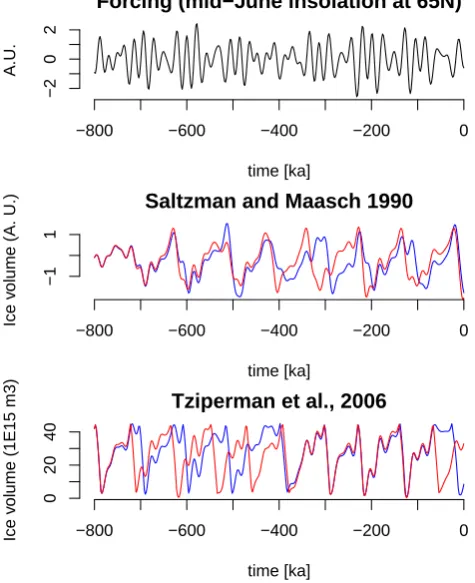
Shown in Fig. 1, for instance, are two further examples of ice volume history reproduced with models previously pub-lished in the palaeoclimate modelling literature (Saltzman and Maasch, 1990; Tziperman et al., 2006). In both cases, small changes in model parameters do, at some stage in the climate history, induce a shift in the sequence of ice ages.

Forcing (mid−June insolation at 65N)

time [ka]

A.U.

−800 −600 −400 −200 0

−2

0

2

Saltzman and Maasch 1990

time [ka]

Ice v

olume (A. U.)

−800 −600 −400 −200 0

−1

1

Tziperman et al., 2006

time [ka]

Ice v

olume (1E15 m3)

−800 −600 −400 −200 0

0

20

40

Fig. 1. Ice volume simulated with two models previously published:

Saltzman and Maasch (1990) and Tziperman et al. (2006), forced by normalised insolation at 65◦N. The blue lines are obtained with the published parameters; the latter were slightly changed to obtain the red ones:p0=0.262 Sv instead of 0.260 Sv in Tziperman et al. (2006), andw=0.6 instead ofw=0.5 in Saltzman and Maasch (1990). While the qualitative aspect of the curves are preserved, the timing of ice ages is affected by the parameter changes.

brought up by Lisiecki (2010) and Rial (2004); Rial et al. (2013).

Tziperman et al. (2006) already observed that a conceptual model fitting the ice age curve is no proof that the correct physical mechanisms have been identified, but is rather an indication of the powerful role of the astronomical forcing as a pacemaker. Our purpose is to take this approach one step further by showing that the powerful action of the astronom-ical forcing as a pacemaker does not guarantee the stability of the ice age sequence.

A first step was proposed in De Saedeleer et al. (2013), where a highly idealised model of ice ages (in essence, a van der Pol oscillator) displays a wide regime of synchronisation when forced to the astronomical forcing. Inspection of the time-averaged largest Lyapunov exponents, as well as basins of attractions, allowed us to conclude that that the forced sys-tem goes through times of unreliable synchronisation, so that the succession of ice ages may sensitively depend on fluctu-ations added to the system.

This work is further developed here in three directions: the role of separate and combined influences of different com-ponents of the astronomical forcing is being analysed more systematically. This allows us to relate the instabilities noted in palaeoclimate models to the literature on quasi-periodic forcings with two components only, and more specifically to the concept of strange non-chaotic attractor. The possibility of synchronisation on eccentricity is also briefly discussed. Second, the effects of additive fluctuations and those of pa-rameter changes are being related qualitatively. Finally, the analysis is applied to six other palaeoclimate models, which provides a better basis to estimate the robustness of the con-clusions.

Providing no conclusions as to whether or not glacial– interglacial cycles are indeed predictable, the present work focuses entirely on the possibility of dynamical stability of simple ice age models. Making conclusions about the real world requires first an elaborate account of the effects asso-ciated with model discrepancy (which is stochastic) that need to be quantified through a process of statistical inference.

2 The van der Pol oscillator 2.1 Model definition

Before going further a word of justification is needed about the use of the van der Pol oscillator as the starting point of this study.

The succession of glaciations and terminations is com-monly understood as a phenomenon of relaxation, during which regimes of linear response to the astronomical forc-ing alternate with non-linear phenomena durforc-ing which the attracting point of the system changes.

The idea, popularised by Paillard (1998), is already im-plicit in the works of Oerlemans (1980), based on experi-ments with an ice sheet-lithosphere model. However, the un-derstanding of the nature of the instabilities that are neces-sary to cause the succession of glacial–interglacial cycles has considerably evolved over time, as it may involve the lithosphere (Oerlemans, 1980), the ocean biogeochemistry (Saltzman et al., 1984), a combination of both (Saltzman and Verbitsky, 1993), the ocean circulation (Paillard and Par-renin, 2004) or sea-ice-atmospheric interactions (Gildor and Tziperman, 2000).

The van der Pol model is thus chosen here as it is one of the simplest relaxation oscillators, without consideration of the exact physical mechanism that causes the ice age oscilla-tions.

It is a dynamical system of two ordinary differential equa-tions:

dx

dt = −

1

τ(F (t )+β+y) .

dy

dt = α τ(y−y

3_/3+x),

with(x, y)as the climate state vector,τ a time constant,α

a time-decoupling factor,βa bifurcation parameter andF (t )

the forcing. The parameterβ does not appear in the original van der Pol equations (van der Pol, 1926), and the present variant is sometimes referred to as the biased van der Pol

model.

The autonomous (i.e. F (t )=0) model displays self-sustained oscillations as long as|β|<1. For later reference the period of the unforced oscillator is denotedTn(τ ). The variablexthen follows a saw-tooth periodic cycle, the asym-metry of which is controlled byβ.

We choseα=30. This choice implies that variabley un-dergoes rapid variations compared tox, and it may therefore be referred to as the “fast” variable. In climate terms,xmay be interpreted as a glaciation index, which slowly accumu-lates the effects of the astronomical forcingF (t ), while y, which shifts between approximately−1 and 1, might be in-terpreted as some representation of the ocean or carbon cycle dynamics.

Again, the van der Pol oscillator is only taken here as a starting point, its representativeness of the physics of ice ages being admittedly contentious. Models with more explicit in-terpretations of ice age physics will be discussed in Sect. 3.

In ice age models the forcing function is generally one or several insolation curves, computed for specific seasons and latitudes. The rationale behind this choice is that whichever insolation is used it is, to a very good approximation, a lin-ear combination of climatic precession and obliquity (Loutre, 1993, see also Appendix A). The choice of one specific inso-lation curve may be viewed as a modelling decision about the effective forcing phase of climatic precession, and the rela-tive amplitudes of the forcings due to precession and obliq-uity. In turn, climatic precession and obliquity can be ex-pressed as a sum of sines and cosines of various amplitudes and frequencies (Berger, 1978), so thatF (t )can be modelled as a linear combination of about a dozen of dominant peri-odic signals, plus a series of smaller amplitude components. They are shown in Fig. 2. More details are given in Sect. 2.4. With these hypotheses the van der Pol model may be tuned so that the benthic curve over the last 800 000 yr is reasonably well reproduced (Fig. 3).

Abundant literature analyses the response of the van der Pol oscillator to a periodic forcing (e.g. Mettin et al., 1993; Guckenheimer et al., 2003, and references therein). The re-sponse of oscillators to the sum of two periodic forcings has been the focus of attention because it leads to the emergence of “strange non-chaotic attractors”, a concept first introduced by Grebogi et al. (1984) and further studied in, among others, Wiggins (1987); Romeiras and Ott (1987); Kapitaniak and Wojewoda (1990, 1993); Belogortsev (1992); Feudel et al. (1997); and Glendinning et al. (2000). To our knowledge, however, there is no systematic study of the response of an oscillator to a signal of the form of the astronomical forc-ing. Le Treut and Ghil (1983), for example, represented the astronomical forcing as a sum of only two or three periodic

0 20 40 60 80 100

Period [ka]

0.0

0.2

0.4

0.6

0.8

1.0

amplitude

Precession

0 20 40 60 80 100

Period [ka]

0.0

0.2

0.4

0.6

0.8

1.0

Obliquity

Fig. 2. Spectral decomposition of precession and obliquity given by

Berger (1978), scaled here such that the strongest components have amplitude 1.

components and it will be shown here that it is worth consid-ering the astronomical forcing with all its complexity. 2.2 Periodic forcing

Consider a sine-wave forcing (F (t )=γsin(2π/P1t+φP1)), with period P1=23 716 yr andφP1=32.01◦. This is the first component of the harmonic development of climatic pre-cession (Berger, 1978). If certain conditions are met – they will soon be given – the van der Pol oscillator may become synchronised on the forcing. Synchronised means, in this par-ticular context, that the response of the system displaysp cy-cles withinqforcing periods, wherepandq are integers. It is said that the system is in ap:q synchronisation regime (Pikovski et al., 2001, p. 66–67). The output is periodic, and its period is equal toq×P1.

−700 −600 −500 −400 −300 −200 −100 0 −1.0 −0.5 0.0 0.5 1.0

van der Pol oscillator forced by astronomical forcing

time [ka]

x

LR04 delta−18 O

● ● ● ● ● ● ● ● ● ● ● ● ● ● ● ● ● ● ● ● ● ● ● ● ● ● ● ● ● ● ● ● ● ● ● ● ● ● ● ● ● ● ● ● ● ● ● ● ● ● ● ● ● ● ● ● ● ● ● ● ● ● ● ● ● ● ● ● ● ● ● ● ● ● ● ● ● ● ● ● ● ● ● ● ● ● ● ● ● ● ● ● ● ● ● ● ● ● ● ● ● ● ● ● ● ● ● ● ● ● ● ● ● ● ● ● ● ● ● ● ● ● ● ● ● ● ● ● ● ● ● ● ● ● ● ● ● ● ● ● ● ● ● ● ● ● ● ● ● ● ● ● ● ● ● ● ● ● ● ● ● ● ● ● ● ● ● ● ● ● ● ● ● ● ● ● ● ● ● ● ● ● ● ● ● ● ● ● ● ● ● ● ● ● ● ● ● ● ● ● ● ● ● ● ● ● ● ● ● ● ● ● ● ● ● ● ● ● ● ● ● ● ● ● ● ● ● ● ● ● ● ● ● ● ● ● ● ● ● ● ● ● ● ● ● ● ● ● ● ● ● ● ● ● ● ● ● ● ● ● ● ● ● ● ● ● ● ● ● ● ● ● ● ● ● ● ● ● ● ● ● ● ● ● ● ● ● ● ● ● ● ● ● ● ● ● ● ● ● ● ● ● ● ● ● ● ● ● ● ● ● ● ● ● ● ● ● ● ● ● ● ● ● ● ● ● ● ● ● ● ● ● ● ● ● ● ● ● ● ● ● ● ● ● ● ● ● ● ● ● ● ● ● ● ● ● ● ● ● ● ● ● ● ● ● ● ● ● ● ● ● ● ● ● ● ● ● ● ● ● ● ● ● ● ● ● ● ● ● ● ● ● ● ● ● ● ● ● ● ● ● ● ● ● ● ● ● ● ● ● ● ● ● ● ● ● ● ● ● ● ● ● ● ● ● ● ● ● ● ● ● ● ● ● ● ● ● ● ● ● ● ● ● ● ● ● ● ● ● ● ● ● ● ● ● ● ● ● ● ● ● ● ● ● ● ● ● ● ● ● ● ● ● ● ● ● ● ● ● ● ● ● ● ● ● ● ● ● ● ● ● ● ● ● ● ● ● ● ● ● ● ● ● ● ● ● ● ● ● ● ● ● ● ● ● ● ● ● ● ● ● ● ● ● ● ● ● ● ● ● ● ● ● ● ● ● ● ● ● ● ● ● ● ● ● ● ● ● ● ● ● ● ● ● ● ● ● ● ● ● ● ● ● ● ● ● ● ● ● ● ● ● ● ● ● ● ● ● ● ● ● ● ● ● ● ● ● ● ● ● ● ● ● ● ● ● ● ● ● ● ● ● ● ● ● ● ● ● ● ● ● ● ● ● ● ● ● ● ● ● ● ● ● ● ● ● ● ● ● ● ● ● ● ● ● ● ● ● ● ● ● ● ● ● ● ● ● ● ● ● ● ● ● ● ● ● ● ● ● ● ● ● ● ● ● ● ● ● ● ● ● ● ● ● ● ● ● ● ● ● ● ● ● ● ● ● ● ● ● ● ● ● ● ● ● ● ● ● ● ● ● ● ● ● ● ● ● ● ● ● ● ● ● ● ● ● ● ● ● ● ● ● ● ● ● ● ● ● ● ● ● ● ● ● ● ● ● ● ● ● ● ● ● ● ● ● ● ● ● ● ● ● ● ● ● ● ● ● ● ● ● ● ●

−700 −600 −500 −400 −300 −200 −100

3.5

4

4.5

5

Time [ka]

Fig. 3. Simulation with the van der Pol oscillator (Eqs. 1–4), forced

by astronomical forcing and compared with the benthic record of Lisiecki and Raymo (2005). Parameters are:α=30,β=0.75,

γp=γo=0.6,τ=36.2 ka.

Each component of the global pullback attractor (two are il-lustrated in Fig. 4b) is a local pullback attractor. Rasmussen (2000, Chap. 2) reviews all the relevant mathematical formal-ism.

In the particular case of a periodic forcing, the strobo-scopic section and the pullback section are often identical (Fig. 5)1.

The number of points on the pullback section may then be estimated for different combinations of parameters and we can use this as a criteria to detect synchronisation. This is done in Fig. 6 for a range ofγ andτ. It turns out that syn-chronisation regimes are organised in the form of triangles, known in the dynamical system literature as Arnol’d tongues (Pikovski et al., 2001, p. 52). Ap:qsynchronisation regime appears when the ratio between the natural period (Tn) and the forcing period is close toq/p. The tolerance, i.e. how distant this ratio can afford to be with respect to q/p, in-creases with the forcing amplitude and dein-creases withpand

q. Synchronisation is weakest (least reliable) near the edge of the tongues. Unreliable synchronisation characterises a sys-tem that is synchronised, but in which small fluctuations may 1_{This property derives from the system invariance with respect} a time translation byP. There will be, however, cases where dif-ferent initial conditions will create difdif-ferent stroboscopic plots. For example two 1:2 synchronisation regimes co-exist in the forced van der Pol oscillator, so that there are four distinct local pullback attractors, while only two points will appear on a stroboscopic plot started from a single set of initial conditions. Rigorously, the global pullback attractor at timetis identical to the global attractor of the iterationt+nP, and the global pullback sections at two timestand

t0are homeomorphic.

(a) x y t P (b) _t 0

t_{back x} y

t

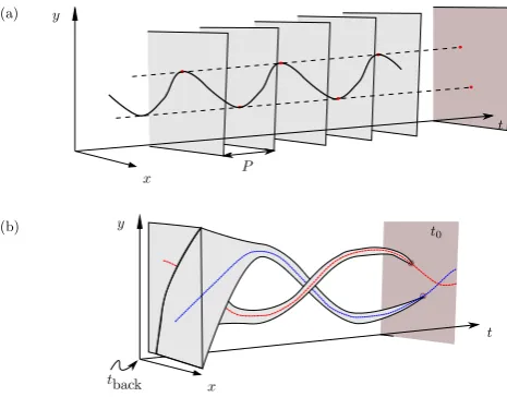
Fig. 4. (a) The stroboscopic section is obtained by superimposing

the system state every forcing period (P), here illustrated for a 2:1 synchronisation. (b) The pullback section at timet0is obtained by superimposing the system states obtained by initialising the system with the ensemble of all possible initial conditions far back in time, here attback. The particular example shows a global pullback attrac-tor made of two local pullback attracattrac-tors (in dashed red and blue), the sections of which are seen att. Also shown is the convergence of initial conditions towards the pullback attractors, in grey.

cause episodes of desynchronisation. In the particular case of periodic forcing the episode of desynchronisation is called a phase slip, as is well explained in Pikovski et al. (2001, p. 54)

Using the pullback attractor to identify synchronisation is not a very efficient method in the periodic forcing case. Arc-length continuation methods are faster and more accurate (e.g. Schilder and Peckham, 2007, and references therein). It is shown, however, in De Saedeleer et al. (2013) that the pull-back section method gives results that are acceptable enough for our purpose, and it is adopted here because it provides a more intuitive starting point to characterise synchronisation with multi-periodic forcings.

2.3 Synchronisation on two periods

Consider now a forcing function that is the sum of two peri-odic signals. Two cases are considered here: the two forcing periods differ by a factor of about 2, and the two forcing pe-riods are close.

2.3.1 P1=23 716 ka andO1=41 000 ka

-1 0_x 1 -2

-1 0 1 2

y

Pullback section

-1 0_x 1

Stroboscopic on

Periodic forcing (

)

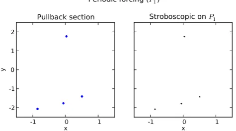
Fig. 5. Pullback (att0=0) and stroboscopic sections (t=0+nP1) obtained with the van der Pol oscillator, with parameters α=

30,β=0.7,τ=36 forced byF (t )=γsin(2π/P1t+φP1),P1= 23.7 ka,φ_P1=32.01◦andγ=0.6. The two plots indicate a case of 4:1 synchronisation, and they are identical because the forcing is periodic.

viewed as a very rough representation of the astronomical forcing.

Let us begin withτ=36 ka, which corresponds to a limit cycle in the van der Pol oscillator of periodTn=98.79 ka, and consider the stroboscopic section onP1(Fig. 7, line 1). Forcing amplitude γ is set to 0.6. Due to the presence of theO1forcing, the four points of the periodic case seen in Fig. 5 have mutated into four local attractors, which appear as closed curves (some are very flat). Every timeP1elapses, the system visits a different local attractor. They are attrac-tors in the sense that they attract solutions of the iteration, bringing the system fromttot+4·P1. In this particular ex-ample, the system is said to be phase- or frequency-locked on

P1with ratio 1:4 (Pikovski et al., 2001, p. 68), because on average, one ice age cycle takes four precession cycles, even though the response is no longer periodic. In this example, the curves on theP1stroboscopic section nearly touch each other. This implies that synchronisation is not reliable since a solution captured by one of these attractors could easily escape and fall into the basin of attraction of another local attractor. One can also see that it is not synchronised onO1 since the stroboscopic section of periodO1shows one closed curve englobing all possible phases. It may also be said that the system is synchronised in the generalised sense (Pikovski et al., 2001, p. 150), because the pullback section is made of only four points: starting from arbitrary conditions, the sys-tem converges to only a small number of solutions at any timet. It is also stable in the Lyapunov sense, a point that will not be further discussed here, but see De Saedeleer et al. (2013).

Consider now τ=41 ka. The four closed curves on the P1-stroboscopic section have collided and merged into one attractor with strange geometry. A similar figure appears on the E1-stroboscopic section. The phenomenon of strange non-chaotic attractor has been described by Grebogi et al.

5 10 15 20 25 30 35 40 45 50

τ

0.2 0.4 0.6 0.8 1.0 1.2 1.4

γ

Periodic forcing (

P

)

1 2 3 4 5

PN/P1

1

2

3

4

5

6

7

> 7

Fig. 6. Bifurcation diagram obtained by counting the number of

points on the pullback section in the van der Pol oscillator (α=30,

β=0.7) andF (t )=γsin(2π/P1t+φP1). The twoxaxes indicate

τand the ratio between the natural system period and the forcing, respectively. One observes the synchronisation regimes correspond-ing to 1:1, 1:2, 1:3, 1:4 and 1:5, respectively (gray, blue, red, green, yellow) and, intertwined, higher order synchronisations in-cluding 3:2, 5:2, 2:3 etc. White areas are weak or no synchro-nisation. Graph constructed usingtback= −10 Ma (see Fig. 11 and text for meaning and implications).

(1984), its occurrence in the van der Pol oscillator is dis-cussed in Kapitaniak and Wojewoda (1990), and its rele-vance to climate dynamics was suggested by Sonechkin and Ivachtchenko (2001). In our specific example, the system is neither frequency-locked onP1nor onO1, but it is synchro-nised in the generalised sense: the pullback section has two points. Finally, withτ=44 ka there is frequency-locking on

O1(regime 3:1) but not onP1.

Clearly, the system underwent changes in synchronisation regimes asτincreased from 36 to 44 ka. Further insight may be had by considering theτ-γ plot (Fig. 8). The frequency-locking regime onP1lies in the relic of the 1:4 tongue vis-ible in the periodic forcing case (Fig. 6). Frequency locking onO1 belongs to the 1:3 tongue associated withO1. The strange non-chaotic regime occurs where the tongues associ-ated with these different forcing components merge.

-2 -1

0 1

2

τ=36 ka

Pullback section Stroboscopic on

Stroboscopic on

-2 -1 0 1 2

τ=41 ka

-1 0 1

-2 -1 0 1 2

τ=44 ka

-1 0 1 -1 0 1

Quasi-periodic forcing (P1+E1)

Fig. 7. Pullback (att0=0) and stroboscopic sections (t=0+nP1 andt=0+nO1) obtained with the van der Pol oscillator with pa-rametersα=30,β=0.7, and forced byF (t )=γ (sin(2π t /P1+

φP1)+sin(2π t /O1)+φO1),P1=23.7 ka andO1=41.0 ka and

γ=0.6, and three different values ofτ. The presence of dots on the pullback section indicates generalised synchronisation. Localised closed curves on the stroboscopic sections indicate frequency lock-ing on the correspondlock-ing period (on P1 with τ=36 ka andO1 withτ=44 ka), and complex geometries indicate the presence of a strange attractor (τ=41 ka).

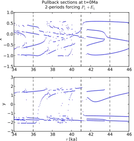
Another view on the bifurcation structure may be obtained by plotting thexandy solutions of the system att0=0, ini-tiated from a grid of initial conditions attback= −5 Ma (Mil-lion years), as a function ofτ, still withγ=0.6 (Fig. 9). This plot outlines a region of sensitive dependence on the input parameter, more specifically betweenτ =37 and 42 ka.

These observations have two important consequences for our understanding of the phenomena illustrated in Fig. 1. To see this it is useful to refer to general considerations about autonomous dynamical systems. A bifurcation generally sep-arates two distinct (technically: non-homeomorphic) attrac-tors, which control the asymptotic dynamics of the system. As the bifurcation is being approached, the convergence to the attractor is slower, while the attractor that exists on the other side of the bifurcation may already take some tempo-rary control on the transient dynamics of the system. This is, namely, one possible mechanism of excitable systems. One sometimes refers to “remnant” or “ghost attractors” to refer to these attractors that exist on the other side of the bifur-cation and may take control on the dynamics of the system over significant time intervals (e.g. Nayfeh and Balachan-dran, 2004, p. 206).

The idea may be generalised to non-autonomous sys-tems. Consider Fig. 10. The upper plot shows the two local

10 15 20 25 30 35 40 45 50

τ

0.0 0.2 0.4 0.6 0.8 1.0 1.2 1.4

γ

1 2 3 4 5

PN/P1

0.5 1.0 1.5 2.0 2.5 3.0

PN/O1

Quasi-periodic forcing (P1 and O1)

Fig. 8. As Fig. 6 but with a 2-period forcing: F (t )=

γ (sin(2π/P1t+φP1)+sin(2π/O1t+φO2))(see text for values). Tongues originating from frequency-locking on individual periods merge and give rise to strange non-chaotic attractors. Orange dots correspond to the cases shown in Fig. 7.

pullback attractors of the system obtained withτ =41 ka. The middle panel displays one local attractor obtained with

τ=40. The twoτ =41 attractors are reproduced with thin lines for comparison. Observe that this τ =40 attractor is qualitatively similar to theτ =41 attractors, and most of its time is spent on a path that is nearly undistinguishable from those obtained with τ=41. However, on a portion of the time interval displayed it follows a sequence of osciliations that is distinct from those obtained withτ =41. In fact, there are four pullback attractors atτ=40.

Let us now consider a third scenario. Parameterτ =41, but an additive stochastic term (σd_dω_t, σ2=0.25ka−1, andω

symbolises a Wiener process) is added to the second system equation. This is thus a slightly noisy version of the original system. Shown here is one realisation of this stochastic equa-tion, among the infinity of solutions that could be obtained with this system. Expectedly, the system spends large frac-tions of time near one or the other of the two pullback attrac-tors. However, it also spends a significant time on a distinct path. Speculatively, this distinct path is under the influence of a “ghost” pullback attractor. As the bifurcation structure is complex and dense, as shown in Fig. 9, we expect a host of ghosts to lie around, ready to take control of the system over significant fractions of time, and this is what happens in this particular case.

34

36

38

40

42

44

46

1.5

1.0

0.5

0.0

0.5

1.0

x

34

36

38

40

42

44

46

τ

[ka]

3

2

1

0

1

2

3

y

Pullback sections at t=0Ma

2-periods forcing

Fig. 9. Pullback solutions of the van der Pol oscillator forced by two

periods (as in Figs. 7 and 8) as a function ofτ. Forcing amplitude isγ=0.6 and the other parameters are as on the previous figures. Vertical lines indicate the cases shown in Fig. 7.

tback. Surprisingly, one needs to go back to−30 Ma to iden-tify the true pullback attractor. Obviously 30 Ma is a very long time compared to the Pleistocene and so this solution is in practice no more relevant than the 4 or 8 solutions that can be identified by only starting the system back in time 1 or 2 Ma ago. They may be interpreted as ghost pullback attrac-tors, and following the preceding discussion they are likely to be visited by a system forced by large enough random ex-ternal fluctuations.

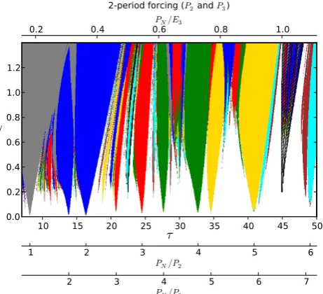
2.3.2 P2=22 427 ka andP3=18 976 ka

The two periods now being combined are the second and third components of precession, still according to Berger (1978). These two periods were selected for two reasons. The first one is that the addition of the two periodic signal pro-duces an interference beating with period 123 319 yr, not too far away from the usual 100 ka cycle that characterises Late Pleistocene climatic cycles. Second, the period of the beating is not close to an integer number of the two original periods (this occurs, accidentally, when usingP1andP3). This was important to be able to clearly distinguish a synchronisation to the beating from a higher resonance harmonic to either forcing components.

It is known from astronomical theory that the periodic-ity of eccentricperiodic-ity is mechanically related to the beatings of the precession signal (Berger, 1978). The scientific question

0 200 400 600 800 1000 1200 1400 1600 1800 1.5

1.0 0.5 0.0 0.51.0

y

pullback attractors

τ

0 200 400 600 800 1000 1200 1400 1600 1800 1.5

1.0 0.5 0.0 0.51.0

y

one pullback attractor

τ

0 200 400 600 800 1000 1200 1400 1600 1800 time [kyr]

1.5 1.0 0.5 0.0 0.51.0

y

one stochastic realisation

τ

Fig. 10. (Top) pullback attractors of the forced van der Pol

oscil-lator (β=0.7,α=30,γ=0.6 with 2-period forcing) as in Fig. 8, forτ=41 ka. They are reproduced on the graphs below (very thin lines), overlain by (middle) one pullback attractor with same pa-rameters butτ=40 ka, and (bottom) one stochastic realisation of the stochastic van der Pol oscillator withτ=41 ka.

considered here is whether the correspondence between the period of ice age cycles and eccentricity is coincidental, or whether a phenomenon of synchronisation of climate on ec-centricity developed.

To address this question we need a marker of synchro-nisation on the precession beating. The Rayleigh number has already been used to this end in palaeoclimate appli-cations (Huybers and Wunsch, 2004; Lisiecki, 2010). Let

Pb be the beating period, and Xi the system state snap-shot every t=t0+iPb, the Rayleigh number R is defined as |P

10

-1

10

0

10

1

10

2

−

t

[Myr]

1

2

4

8

# of distinct solutions at

t

₀

=0

Fig. 11. Number of distinct solutions simulated with the van der Pol

oscillator (β=0.7,α=30,τ=41 ka andγ=0.6 with 2-period forcing as in Fig. 8, as a function of the timetback at which 121 distinct initial conditions are considered. The actual stable pullback attracting set(s), in the rigorous mathematical sense, is (are) found fortback→ −∞.

sensitivity experiments show that convergence is quite slow. More specifically, the synchronisation diagram was com-puted here using tback= −10 Ma. With shorter backward time horizons, the number of remaining solutions identified in the beating-synchronisation regime often exceeds 6 and could not be seen on the graph, while the Rayleigh number was still beyond 0.95. Hence, a high Rayleigh number is not necessarily a good indicator of reliable synchronisation. 2.4 Full astronomical forcing

The next step is to consider the full astronomical forcing, as the sum of standardised climatic precession (5) and the deviation of obliquity with respect to its standard value (O):

F (t )=γp5(t )+γoO(t ), (2)

where

5(t )=

Np

X

i=1

aisin(ωpit+φpi)/a1 (3)

O=

No

X

i=1

bicos(ωoit+φoi)/b1. (4)

The various coefficients are taken from Berger (1978). We takeNp=No=34, so that the signal includes in total 68 harmonic components. With this choice the BER78 solu-tion (Berger, 1978) is almost perfectly reproduced. BER78 is

10 15 20 25 30 35 40 45 50

τ

0.0 0.2 0.4 0.6 0.8 1.0 1.2

γ

1 2 3 4 5 6

PN/P2

2 3 4 5 6 7

PN/P3

0.2 0.4 0.6PN/E3 0.8 1.0 2-period forcing (P2 and P3)

Fig. 12. As Fig. 8 but with: F (t )=γ (sin(2π/P2t+φP2)+ sin(2π/P3t+φP3)). Hashes indicate regions of Rayleigh number

>0.95 on the beating associated withP2 andP3, the period of which is calledE3in the Berger (1978) nomenclature (third com-ponent of eccentricity).

still used in many palaeoclimate applications. Compared to a state-of-the-art solution such as La04 (Laskar et al., 2004), the error on amplitude is between 0 and 25 %, and the error on phase is generally much less than 20◦.

The bifurcation diagram representing the number of pull-back solutions as a function of forcing amplitude and τ is shown in Fig. 13. We have takenγ=γp=γo. One recog-nises the tongues originating from the individual components merging gradually into a complex pattern. The number of at-tractors settles to 1 as the amplitude of the forcing is further increased. Let us call this the 1-pullback attractor regime. We already know that synchronisation is generally not reliable in the region characterised by the complex and dense bifurca-tion region, where more than one attractor exist. The remain-ing problem is to characterise the reliability of synchronisa-tion in the 1-pullback attractor regime.

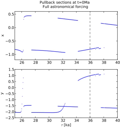
The literature says little about systematic approaches to quantify the reliability of generalised synchronisation with quasi-periodic forcings. To develop further the ideas devel-oped in Sect. 2.3.1, one can plot pullback solutions at a cer-tain timet as a function of one or several parameters. This is done in Fig. 14. Hereγ is kept constant (= 1.0) andτ is varied between 25 and 40. There is a brief episode of a 2-solution regime between 31 and 32 ka. Within the 1-2-solution regime there is a number of abrupt transitions (at 26, 27, 34 and 37 ka).

10 15 20 25

τ

0.4 0.6 0.8 1.0 1.2 1.4

γ

Full astronomical forcing

Fig. 13. As Fig. 8 but with the full astronomical forcing, made of

34 precession and 34 obliquity periods (Eq. 2).

could be verified up to machine precision. The abrupt vari-ation at τ =37.59. . . appears numerically as a continuous variation of the attractor spread over an interval of 10−7_ka2_. Further work is required to understand the origin of these discontinuities, and in particular to understand to what extent they relate to the strange nature of the attractor. The relevant aspect in the present context is that these discontinuities in-duce similar phenomena as those described in Sect. 2: the presence of ghost attractors and sensitive dependence to fluc-tuations. Hence, being in the 1-pullback attractor regime does not guarantee a reliable synchronisation on the astronomical forcing. One needs to be deep into that zone.

3 Other models

We now consider 6 previously published models. Mathemat-ical details are given in the Appendix and the codes are avail-able online at https://github.com/mcrucifix.

– SM90: this is a model with three ordinary differen-tial equations representing the dynamics of ice volume, carbon dioxide concentration and deep-ocean temper-ature. The astronomical forcing is linearly introduced in the ice volume equation, under the form of inso-lation at 65◦N on the day of summer solstice. Only the carbon dioxide equation is linear, and this non-linearity induces the existence of a limit-cycle solution – spontaneous glaciation and deglaciation – in the cor-responding autonomous system. The SM90 model is 2_{Note also that at least one discontinuity up to machine precision} could also be identified in the 1-pullback attractor regime whenα=

1, which suggests that the feature is not conditioned by the slow-fast character of the system.

Fig. 14. As Fig. 9 but with the full astronomical forcing, with

pa-rameters as in Fig. 13 andγ=1.0.

thus a mathematical transcription of the hypothesis ac-cording to which the origin 100 000 yr cycle is to be found in the biological components of Earth’s climate. – SM91: this model is identical to SM90 except for a

dif-ference in the carbon cycle equation.

– PP04: the Paillard–Parrenin model (Paillard and Par-renin, 2004) is also a 3-differential-equation system, featuring Northern Hemisphere ice volume, Antarctic ice area and carbon dioxide concentration. The carbon dioxide equation includes one non-linear term asso-ciated to a switch on/off of the Southern Ocean ven-tilation. Astronomical forcing is injected linearly at three places in the model: in the ice-volume equation, in the carbon dioxide equation, and in the ocean ven-tilation parameterization. The autonomous version of the model also features a limit cycle. As in SM90 and SM91 the non-linearity introduced in the carbon cycle equation plays a key role but the bifurcation structure of this model differs from SM90 and SM91 (Crucifix, 2012).

which is the combination of a differential equation in which the astronomical forcing is introduced linearly as a summer insolation forcing term, and a discrete variable, which may be 0 or 1 to represent the absence or presence of sea ice in the Northern Hemisphere. – I11: the Imbrie et al. (2011) was introduced by its

au-thors as a “phase-space” model. It is a 2-D model, for which the equations were designed to distinguish an “ice accumulation phase” and an “abrupt deglacia-tion” phase, which is triggered when a threshold de-fined in the phase space is crossed. I11 was specifically tuned to reproduce the phase-space characteristics of the benthic oxygen isotopic dynamics. A particularity of this model is that the phasing and amplitude of the forcing depend on the level of glaciation.

– PP12: similar to Imbrie et al. (2011), the Parrenin and Paillard (2012) model distinguishes accumula-tion and deglaciaaccumula-tion phases. Accumulaaccumula-tion is a lin-ear accumulation of insolation, without restoring force (hence similar to Eq. (1) of the van der Pol oscilla-tor); deglaciation accumulates insolation forcing but a negative relaxation towards deglaciation is added. Contrary to Imbrie et al. (2011), the trigger function, which determines the regime change, is mainly a func-tion of astronomical parameters. An ice volume term only appears in the function controlling the shift from “accumulation” to “deglaciation” regime.

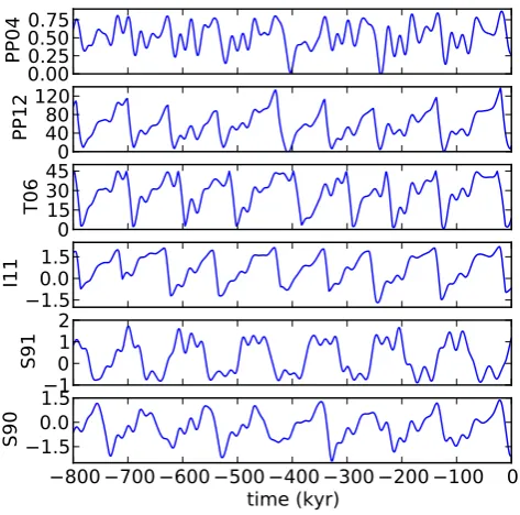
The ice volumes (or, equivalently, glaciation index or sea level) simulated by each of these models are shown in Fig. 15. Shown here are estimates of the pullback attractors; more specifically, the trajectories obtained with an ensem-ble of initial conditions at tback= −20 Ma. In some cases the curves actually published (in particular in SM90) are not pullback attractors, but ghost trajectories in the sense illus-trated in Fig. 11. In some cases (PP04 and PP12) the param-eters had to be slightly adjusted to reproduce the published version satisfactorily. Details are given in Appendix.

Some of these models include as much as 14 adjustable parameters (e.g.: PP04) and a full dynamical investigation of each of them is beyond the scope of the study. Rather, we proceed as follows. Every model responds to a state equa-tion, which may be written, in general (assuming a numerical implementation), as

ti+1=ti+δt

xi+1=xi+δt f (xi, F (ti)),

whereti is the discretised time,xi the climate state (a 2-D or 3-D vector) atti andF (ti)is the astronomical forcing, which is specific to each model because the different authors made different choices about the respective weights and phases of precession and obliquity.

0.00

0.25

0.50

0.75

PP04

0

40

80

120

PP12

0

15

30

45

T06

1.5

0.0

1.5

I11

1

0

1

2

S91

800 700 600 500 400 300 200 100 0

time (kyr)

1.5

0.0

1.5

S90

Fig. 15. Pullback attractors obtained for 6 models over the last

800 ka, forced by astronomical forcing with the parameters of the original publications. Shown is the model component representing ice volume. Units are arbitrary in all models, except in T06 (ice volume in 1015m3) and PP12 (sea-level equivalent, in m).

In all generality, the equation (or its numerical approxima-tion) may be rewritten as follows, posingτ =1 andγ =1:

ti+1=ti+δt

xi+1=xi+ 1

τδt f (xi, γ F (ti)).

The parametersτ andγ introduced this way have a similar meaning as in the van der Pol oscillator, sinceτ controls the characteristic response time of the model, whileγ controls the forcing amplitude.

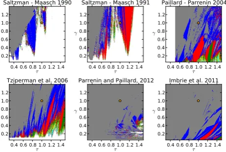
Bifurcation diagrams, similar to Fig. 13 are then shown in Fig. 16. Remember thatγ=τ =1 corresponds to the model as originally published.

0.4 0.6 0.8 1.0 1.2 1.4

τ

0.2 0.4 0.6 0.81.0 1.2

γ

Saltzman - Maasch 1990

0.4 0.6 0.8 1.0 1.2 1.4

τ

0.2 0.4 0.6 0.81.0 1.2

γ

Saltzman - Maasch 1991

0.4 0.6 0.8 1.0 1.2 1.4

τ

0.2 0.4 0.6 0.81.0 1.2

γ

Paillard - Parrenin 2004

0.4 0.6 0.8 1.0 1.2 1.4

τ

0.2 0.4 0.6 0.81.0 1.2

γ

Tziperman et al. 2006

0.4 0.6 0.8 1.0 1.2 1.4

τ

0.2 0.4 0.6 0.81.0 1.2

γ

Parrenin and Paillard, 2012

0.4 0.6 0.8 1.0 1.2 1.4

τ

0.2 0.4 0.6 0.81.0 1.2

γ

Imbrie et al. 2011

Fig. 16. As Fig. 13 but for 6 models previously published. Orange

dots correspond to standard (published) parameters of these models.

experimenting with this model shows that instabilities such as displayed in Fig. 1 are harder to obtain.

I11, with standard parameters, is also fairly deep in the stable zone. One has to consider much smaller forcing val-ues than published to recognise the synchronisation tongue structure that characterises oscillators (Fig. 17).

PP12 finally turns out to be the only case not showing a tongue-like structure. This may be surprising because this model also has limit-cycle dynamics (self-sustained oscilla-tions in the absence of astronomical forcing). Some aspects of its design resemble the van der Pol oscillator. The role of the variabley in the van der Pol oscillator is here played by the mode, which may either beg(glaciation) ord (deglacia-tion). Also similar to the van der Pol, the direct effect of the astronomical forcing on the ice volume (xin the van der Pol;

v in PP04) is additive. T06 has also similar characteristics. The distinctive feature of PP12 is that the transition between deglaciation and glaciation modes is controlled by the astro-nomical forcing and not by the system state, as in the other models. To assess the importance of this element of design we considered a hacked version of PP12, where thed→g

occurs when forv < v1(cf. Appendix B6 for model details). In this case the tongue synchronisation structure is recovered, with standard parameters marginally in the reliable synchro-nisation regime (Fig. 17).

4 Conclusions

The present article is built around the paradigm of the “pace-maker”, that is, the timing of ice ages arises as a combination of climate’s internal dynamics with the variations of incom-ing solar radiation induced by the variations of our planet’s orbit and obliquity. Mathematically, this implies that the models of ice ages tested here either present self-sustained oscillations in absence of astronomical forcing, or that the structure of the vector field is organised such as to excite

0.6 0.8 1.0 1.2 1.4

τ

0.00 0.02 0.04 0.06 0.08 0.10 0.12 0.14

γ

Imbrie et al. 2011

0.6 0.8 1.0 1.2 1.4

τ

0.0 0.2 0.4 0.6 0.8 1.0 1.2 1.4

γ

Parrenin and Paillard, 2012 (*)

Fig. 17. As Fig. 16 for (left) the I11 model, but with a zoom on thex

axis, and (right) for a slightly modified version of the PP12 model, in which the transition between deglacial and glacial states is also controlled by ice volume, as opposed to the original PP12 model.

cyclic dynamics in the presence of a forcing. Once the forc-ing is present, the two scenarios will result in qualitatively similar dynamics (see Crucifix, 2012, for more discussion on this point).

In this study we paid attention to the dynamical aspects that may affect the stability of the ice age sequence and its predictability. First, the astronomical forcing has a rich har-monic structure. We showed that a system like the van der Pol oscillator is more likely to be synchronised on the astronom-ical forcing (as nature provides it) than on a periodic forcing, because the fraction of the parameter space corresponding to synchronisation is larger in the former case. A synchronised system is Lyapunov stable, so that at face value this would imply that the sequence of ice ages is stable. However, – this is the second point – even if the dynamical structure of the Pleistocene climate was correctly identified, there would be at least two sources of uncertainty : random fluctuations as-sociated with the chaotic atmosphere and ocean and other statistically random forcings like volcanoes; and uncertainty on system parameters. In theory both types of uncertainties point to different mathematical concepts: path-wise stabil-ity to random fluctuations in the first case, and the structural stability in the second. In practice, however, lack of either form of stability will result in similar consequences: quan-tum skips of insolation cycles in the succession of ice ages. This was the lesson of Fig. 10.

It was shown here that, compared to periodic forcing, the richness of the harmonic structure of astronomical forcing favours situations of weak structural stability. The interpre-tation of the phenomenon relates directly to the theory of quasi-periodically forced dynamical systems, and the insta-bility develops under relatively weak forcing. It is to be dis-tinguished from the chaos known to develop at high forcing amplitude, and which has been implied in El-Niño theories Tziperman et al. (1994).

select the most plausible model on the sole basis of our knowledge of physics, biology and chemistry. Consequently, while we have understood here how and why the sequence of ice ages could be unstable in spite of available evidence (astronomical spectral signature; Rayleigh number), estimat-ing the stability of the sequence ice ages and quantifyestimat-ing our ability to predict ice ages is also a problem of statistical in-ference: calibrating and selecting stochastic dynamical sys-tems based on both theory and observations, which are sparse and characterised by chronological uncertainties. A conclu-sive demonstration of our ability to reach this objective is still awaited.

Appendix A Insolation

In the following models, the forcing is computed as a sum of precession (5=esin$ /a1), co-precession (5˜ = ecos$ /a1) and obliquity (O=(ε−ε0)/b1) computed ac-cording to the Berger (1978) decomposition (Fig. 2, and Eqs. 3–4). More precisely, we use here these quantities scaled (P,5˜ andO) such as they have unit variance. All insolation quantities used in climate models may be approximated as a linear combination of5,5˜ andO. For example:

– normalised summer solstice insolation at 65◦N = 0.89495+0.4346O

– normalised insolation at 60◦S on the 21 February =

−0.49425+0.83995˜ +0.2262O.

Appendix B Model definitions B1 SM90 model

dx

dt = −x−y−v z−uF (t )

dy

dt = −pz+r y+s z

3_{−w y z−z}2_y

dz

dt = −q (x+z)

p=1.0,q=2.5,r=0.9,s=1.0,u=0.6,v=0.2 andw=

0.5, andF (t )is (here) insolation on the day of summer sol-stice, at 65◦_{N, normalised (results are qualitatively} insensi-tive to the exact choice of insolation).

B2 SM91 model

dx

dt = −x−y−v z−uF (t )

dy

dt = −pz+r y−s y 2_−y3

dz

dt = −q(x+z)

p=1.0,q=2.5,r=1.3,s=0.6,u=0.6 andv=0.2, and

F (t )is (here) insolation on the day of summer solstice, at 65◦N, normalised (results are qualitatively insensitive to the exact choice of insolation). One time unit is 10 ka.

B3 PP04 model

The three model variables areV (Ice volume),A(Antarctic Ice Area) andC(Carbon dioxide concentration):

dV

dt =

1

τV

(−xC−yF1(t )+z−V )

dA

dt =

1

τA

(V−A)

dC

dt =

1

τC

(αF1(t )−βV+γ H+δ−C),

τV =15 ka, τC=5 ka, τA=12 ka, x=1.3, y=0.4 (was 0.5 in the original paper),z=0.8,α=0.15,β=0.5,γ =

0.5,δ=0.4,a=0.4,b=0.7,c=0.01,d=0.27;H=1 if

aV−bA+d−c F2(t ) <0, andH=0 otherwise.F1(t )is the normalised, summer-solstice insolation at 65◦_{N, andF}

2(t )is insolation at 60◦_{S on the 21 February (taken as 330}◦_{of true} solar longitude). Other quantities (V, A,C) have arbitrary units.

B4 T06 model

The two model variables arex (ice volume) andy (sea-ice area).xis expressed in units of 1015m3.

dx

dt =(p0−K x)(1−αsi)−(s+smF (t ))

The equation represents the net ice balance, as accumula-tion minus ablaaccumula-tion, and αsi is the sea-ice albedo. αsi= 0.46y.yswitches from 0 to 1 whenxexceeds 45×106_km3_, and switches from 1 to 0 when x decreases below 3×

B5 I11 model Define first:

φ= π

180· (

10−25y wherey <0,

10 elsewhere. (B1)

θ=

(

0.135+0.07y wherey <0,

0.135 elsewhere.

a=0.07+0.015y hO=(0.05−0.005y)O

h5=a5sinφ

h₅˜ =a5˜ cosφ

F =h5+h₅˜ +hO

d= −1+3(F+0.28) 0.51 With these definitions:



 

  ¨

y=0.5[0.0625(d−y)− y˙2

d−y] wherey > θ,˙

˙

y= −0.036375+y[0.014416+y(0.001121

−0.008264y)] +0.5F elsewhere,

(B2)

wherey˙=dy

dt andy¨=

dy˙

dt. Note that the polynomial on the right-hand side of the equation fory˙is a continuous fit to the piece-wise function used in the original Imbrie et al. (2011) publication. Time units are here ka.

B6 PP12 model

This is a hybrid dynamical system, with ice volumev (ex-pressed inmof equivalent sea level) and state, which may be

g(glaciation) ord(deglaciation). Define first

f (x):=

(

x+ √

4a2_+x2_{−2a wherex >0,}

x elsewhere.

witha=0.68034. Then define the following quantities, stan-dardised as follows:

5∗=(f (5)−0.148)/0.808

˜

5∗=(f (5)˜ −0.148)/0.808

the thresholdθ=k55+k₅˜5˜+kOO, and finally the follow-ing rule controllfollow-ing the transition between stategandd: (

d→g ifθ < v1 g→d ifθ+v < v0

.

Ice volumev, expressed in sea-level equivalent, responds to the following equation:

dv

dt = −a55

∗_−a ˜ 55˜

∗_−a OO˜+

(

ad−v/τ if state isd

ag if state isg, with the following parameter values: a5=1.456 m ka−1,

a₅˜ =0.387 m ka−1,aO=1.137 m ka−1,ag=0.978 m ka−1,

ad= −0.747 m ka−1, τ=0.834 ka, k5=14.635 m,

k₅˜ =2.281 m, kO=23.5162 m, v0=122.918 m and v1=3.1031 m. This parameter set is the one originally presented by Parrenin and Paillard in Climate of the Past Discussion (which differs from the final version in Climate of the Past), except that kO is 18.5162 m in the original paper. This modification was needed to reproduce the exact sequence of terminations shown by the authors. Subtle details, such as the numerical scheme or the choice of the astronomical solution might explain the difference.

All codes and scripts are available from GitHub at https: //github.com/mcrucifix.

Addendum

The recently published article by Mitsui and Aihara (2013) further discusses this topic, by providing further support to the existence of strange non-chaotic attractors in van der Pol model as well as SM90, SM91 and PP04. They discuss also the question of sensitive dependence to fluctuations and their connection with the occurrence of strange non-chaotic attrac-tors, with references to the works of Khovanov et al. (2000) in addition to those cited here.

Acknowledgements. Thanks are due to Peter Ditlevsen (Niels

Bohr Institute, Copenhague), Frédéric Parrenin (Laboratoire de Glaciologie et de Géophysique, Grenoble), Bernard De Saedeleer, Ilya Ermakov and Guillaume Lenoir (Université catholique de Louvain) for comments on an earlier version of this manuscript. Two anonymous reviewers as well as Takahito Mitsui (FIRST, Aihara Innovative Mathematical Modelling Project, and University of Tokyo) provided useful comments that improved the Climate of the Past Discussion version. Thanks are also due to the numerous benevolent developers involved in the R, numpy and matplotlib projects, without which this research would have taken far more time. MC is research associate with the Belgian National Fund of Scientific Research. This research is a contribution to the ITOP project, ERC-StG grant 239604.

References

Belogortsev, A. B.: Quasiperiodic resonance and bifurcations of tori in the weakly nonlinear duffing oscillator, Physica D, 59, 417– 429, doi:10.1016/0167-2789(92)90079-3, 1992.

Berger, A.: Support for the astronomical theory of climatic change, Nature, 268, 44–45, doi:10.1038/269044a0, 1977.

Berger, A. L.: Long-term variations of daily insolation and Quaternary climatic changes, J. Atmos. Sci., 35, 2362–2367, doi:10.1175/1520-0469(1978)035<2362:LTVODI>2.0.CO;2, 1978.

Crucifix, M.: Oscillators and relaxation phenomena in Pleis-tocene climate theory, Philos. T. R. Soc. A, 370, 1140–1165, doi:10.1098/rsta.2011.0315, 2012.

De Saedeleer, B., Crucifix, M., and Wieczorek, S.: Is the as-tronomical forcing a reliable and unique pacemaker for cli-mate? A conceptual model study, Clim. Dynam., 40, 273–294, doi:10.1007/s00382-012-1316-1, 2013.

Feudel, U., Grebogi, C., and Ott, E.: Phase-locking in quasiperiodically forced systems, Phys. Rep., 290, 11–25, doi:10.1016/S0370-1573(97)00055-0, 1997.

Gildor, H. and Tziperman, E.: Sea ice as the glacial cycles climate switch: role of seasonal and orbital forcing, Paleoceanography, 15, 605–615, doi:10.1029/1999PA000461, 2000.

Grebogi, C., Ott, E., Pelikan, S., and Yorke, J. A.: Strange attractors that are not chaotic, Physica D:, 13, 261–268, 1984.

Glendinning, P., Feudel, U., Pikovsky, A. S., and Stark, J.: The structure of mode-locked regions in quasi-periodically forced circle maps, Physica D, 140, 227–243, doi:10.1016/S0167-2789(99)00235-3, 2000.

Guckenheimer, J., Hoffman, K., and Weckesser, W.: The forced van der Pol Equation I: the slow flow and its bifurcations, SIAM J. Appl. Dynam. Sys., 2, 1–35, doi:10.1137/S1111111102404738, 2003.

Hays, J. D., Imbrie, J., and Shackleton, N. J.: Variations in the Earth’s orbit: pacemaker of ice ages, Science, 194, 1121–1132, doi:10.1126/science.194.4270.1121, 1976.

Huybers, P. and Wunsch, C.: A depth-derived Pleistocene age model: uncertainty estimates, sedimentation variability, and nonlinear climate change, Paleoceanography, 19, PA1028, doi:10.1029/2002PA000857, 2004.

Imbrie, J. and Imbrie, J. Z.: Modelling the climatic re-sponse to orbital variations, Science, 207, 943–953, doi:10.1126/science.207.4434.943, 1980.

Imbrie, J. Z., Imbrie-Moore, A., and Lisiecki, L. E.: A phase-space model for Pleistocene ice volume, Earth Planet. Sc. Lett., 307, 94–102, doi:10.1016/j.epsl.2011.04.018, 2011.

Kapitaniak, T. and Wojewoda, J.: Strange non-chaotic attractors of a quasi-periodically forced van der Pol’s oscillator, J. Sound Vib., 138, 162–169, 1990.

Kapitaniak, T. and Wojewoda, J.: Attractors of Quasiperiodically Forced Systems, chap. 3, Strange Nonchaotic attractors, Wold Scientific publishing, 15–57, Singapore, 1993.

Khovanov, I. A., Khovanova, N. A., McClintock, P. V. E., and Anishchenko, V. S.: The effect of noise on strange nonchaotic attractors, Phys. Lett. A, 268, 315–322, doi:10.1016/S0375-9601(00)00183-3, 2000.

Laskar, J., Robutel, P., Joutel, F., Boudin, F., Gastineau, M., Cor-reia, A. C. M., and Levrard, B.: A long-term numerical solution

for the insolation quantities of the Earth, Astron. Astrophys., 428, 261–285, doi:10.1051/0004-6361:20041335, 2004.

Le Treut, H. and Ghil, M.: Orbital forcing, climatic interac-tions and glaciation cycles, J. Geophys. Res., 88, 5167–5190, doi:10.1029/JC088iC09p05167, 1983.

Lisiecki, L. E.: Links between eccentricity forcing and the 100 000-year glacial cycle, Nat. Geosci., 3, 349–352, doi:10.1038/ngeo828, 2010.

Lisiecki, L. E. and Raymo, M. E.: A Pliocene-Pleistocene stack of 57 globally distributed benthicδ18O records, Paleoceanography, 20, PA1003, doi:10.1029/2004PA001071, 2005.

Loutre, M. F.: Paramètres orbitaux et cycles diurne et saisonnier des insolations, PhD thesis, Université catholique de Louvain, Louvain-la-Neuve, Belgium, 1993.

Mettin, R., Parlitz, U., and Lauteborn, W.: Bifurcation structure of the driven Van der pol oscillator, Int. J. Bifurcat. Chaos, 3, 1529– 1555, doi:10.1142/S0218127493001203, 1993.

Nayfeh, A. H. and Balachandran, B.: Applied Nonlinear Dynamics: Analytical, Computational, and Experimental Methods, Physics Textbook, Wiley-VCH Verlag, Weinheim, Germany, 2004. Oerlemans, J.: Model experiments on the 100,000-yr glacial cycle,

Nature, 287, 430–432, doi:10.1038/287430a0, 1980.

Mitsui, T. and Aihara, K.: Dynamics between order and chaos in conceptual models of glacial cycles, Clim. Dynam., online first, doi:10.1007/s00382-013-1793-x, 2013.

Paillard, D.: The timing of Pleistocene glaciations from a sim-ple multisim-ple-state climate model, Nature, 391, 378–381, doi:10.1038/34891, 1998.

Paillard, D.: Glacial Cycles: toward a New Paradigm, Rev. Geo-phys., 39, 325–346, doi:10.1029/2000RG000091, 2001. Paillard, D. and Parrenin, F.: The Antarctic ice sheet and the

trig-gering of deglaciations, Earth Planet. Sc. Lett., 227, 263–271, doi:10.1016/j.epsl.2004.08.023, 2004.

Saltzman, B. and Verbitsky, M. Y.: Multiple instabilities and modes of glacial rhythmicity in the plio-Pleistocene: a general the-ory of late Cenozoic climatic change, Clim. Dynam., 9, 1–15, doi:10.1007/BF00208010, 1993.

Parrenin, F. and Paillard, D.: Terminations VI and VIII (∼530 and

∼720 kyr BP) tell us the importance of obliquity and preces-sion in the triggering of deglaciations, Clim. Past, 8, 2031–2037, doi:10.5194/cp-8-2031-2012, 2012.

Pikovski, A., Rosenblum, M., and Kurths, J.: Synchronization: a Universal Concept in Nonlinear Sciences, Vol. 12, Cambridge Nonlinear Science Series, Cambridge University Press, New York, 2001.

Rasmussen, M.: Attractivity and Bifurcation for Nonautonomous Dynamical Systems, no. 1907 in Lecture Notes in Mathematics, Springer, Berlin Heidelberg, 2000.

Rial, J.: Earth’s orbital eccentricity and the rhythm of the Pleis-tocene ice ages: the concealed pacemaker, Global Planet. Change, 41, 81–93, doi:10.1016/j.gloplacha.2003.10.003, 2004. Rial, J. A., Oh, J., and Reischmann, E.: Synchronization of the cli-mate system to eccentricity forcing and the 100,000-year prob-lem, Nat. Geosci., 6, 289–293,doi:10.1038/ngeo1756, 2013. Romeiras, F. J. and Ott, E.: Strange nonchaotic attractors of the

Saltzman, B. and Maasch, K. A.: A first-order global model of late Cenozoic climate, T. RSE Earth, 81, 315–325, doi:10.1017/S0263593300020824, 1990.

Saltzman, B. and Maasch, K. A.: A first-order global model of late Cenozoic climate – Part. II: Further analysis based on a sim-plification of the CO2 dynamics, Clim. Dynam., 5, 201–210, doi:10.1007/BF00210005, 1991.

Saltzman, B., Hansen, A. R., and Maasch, K. A.: The late Qua-ternary glaciations as the response of a 3-component feedback-system to Earth-orbital forcing, J. Atmos. Sci., 41, 3380–3389, 1984.

Schilder, F. and Peckham, B. B.: Computing Arnol’d tongue scenarios, J. Comput. Phys., 220, 932–951, doi:10.1016/j.jcp.2006.05.041, 2007.

Sonechkin, D. M. and Ivachtchenko, N. N.: On the Role of a quasiperiodic forcing in the interannual and interdecadal cli-mate variations, CLIVAR exchanges, 6, 5–6, 2001.

Tziperman, E., Stone, L., Cane, M. A., and Jarosh, H.: El-Niño Chaos: Overlapping of resonances between the seasonal cycle and the pacific ocean-atmosphere oscillator, Science, 264, 72– 74, doi:10.1126/science.264.5155.72, 1994.

Tziperman, E., Raymo, M. E., Huybers, P., and Wunsch, C.: Conse-quences of pacing the Pleistocene 100 kyr ice ages by nonlinear phase locking to Milankovitch forcing, Paleoceanography, 21, PA4206, doi:10.1029/2005PA001241, 2006.

Weertman, J.: Milankovitch solar radiation variations and ice age ice sheet sizes, Nature, 261, 17–20, 1976.

van der Pol, B.: On “relaxation-oscillations”, The London, Edin-burgh and Dublin, Philosophical Magazine Series 7, 2, 978–992, November, 1926.