Projecting Antarctic ice discharge using response functions from SeaRISE ice-sheet models

(1)

www.earth-syst-dynam.net/5/271/2014/ doi:10.5194/esd-5-271-2014

Projecting Antarctic ice discharge using response

functions from SeaRISE ice-sheet models

A. Levermann1,2, R. Winkelmann1, S. Nowicki3, J. L. Fastook4, K. Frieler1, R. Greve5, H. H. Hellmer6, M. A. Martin1, M. Meinshausen1,7, M. Mengel1, A. J. Payne8, D. Pollard9, T. Sato5, R. Timmermann6,

W. L. Wang3, and R. A. Bindschadler3

1_{Potsdam Institute for Climate Impact Research, Potsdam, Germany} 2_{Institute of Physics, Potsdam University, Potsdam, Germany}

3_{Code 615, Cryospheric Sciences Laboratory, NASA Goddard Space Flight Center, Greenbelt MD 20771 USA} 4_{Computer Science/Quaternary Institute, University of Maine, Orono, ME 04469, USA}

5_{Institute of Low Temperature Science, Hokkaido University, Sapporo 060-0819, Japan} 6_{Alfred Wegener Institute, Bremerhaven, Germany}

7_{School of Earth Sciences, The University of Melbourne, 3010 Melbourne, Australia} 8_{Bristol Glaciology Centre, University of Bristol, University Road, Clifton, Bristol BS8 1SS, UK} 9_{Earth and Environmental Systems Institute, Pennsylvania State University, University Park, PA 16802, USA}

Correspondence to: A. Levermann (anders.levermann@pik-potsdam.de)

Received: 30 November 2013 – Published in Earth Syst. Dynam. Discuss.: 13 December 2013 Revised: 28 May 2014 – Accepted: 26 June 2014 – Published: 14 August 2014

(2)

1 Introduction

The future evolution of global mean and regional sea level is important for coastal planning and associated adaptation measures (e.g. Hallegatte et al., 2013; Hinkel et al., 2014; Marzeion and Levermann, 2014). The Fourth Assessment Report (AR4) of the Intergovernmental Panel on Climate Change (IPCC) provided sea-level projections explicitly ex-cluding changes in dynamic ice discharge, i.e. additional ice flow across the grounding line, from both Greenland and Antarctica (Alley et al., 2007). These contributions might however be significant for the next century, which would in-fluence global mean (Van den Broeke et al., 2011) as well as regional sea-level changes (Mitrovica et al., 2009), especially since contribution from the ice sheets is clearly relevant on longer timescales (Levermann et al., 2013). While the part of the ice sheet directly susceptible to warming ocean waters on Greenland is limited, marine ice sheets in West Antarc-tica alone have the potential to elevate sea level globally by several metres (Bamber et al., 2009). Previous projections of the Antarctic ice-sheet mass balance have used fully cou-pled climate–ice-sheet models (e.g. Huybrechts et al., 2011; Vizcaíno et al., 2009). These simulations include feedbacks between the climate and the ice sheet and thereby provide very valuable information especially on a multi-centennial timescale. However, on shorter (i.e. decadal to centennial) timescales, the direct climatic forcing is likely to dominate the ice-sheet evolution compared to the feedbacks between ice dynamics and the surrounding climate. For 21st cen-tury projections it is thus appropriate to apply the output of comprehensive climate models as external forcing to the ice sheet, neglecting feedbacks while possibly improving on the accuracy of the forcing anomalies. Here we follow this ap-proach.

In order to meet the relatively high standards that are set by climate models for the oceanic thermal expansion and glacier and ice-cap models which use the full range of state-of-the-art climate projections, it is desirable to use a set of different ice-sheet models to increase the robustness of the projections of Antarctica’s future sea-level contribution. While changes in basal lubrication and ice softening from surface warming and changes in surface elevation through altered precipitation can affect dynamic ice discharge from Antarctica, changes in basal melt underneath the ice shelves are here assumed to be the dominant driver of changes in dynamic ice loss.

Here we combine the dynamic response of five differ-ent Antarctic sheet models to changes in basal ice-shelf melt with the full uncertainty range of future climate change for each of the Representative Concentration Path-ways (RCPs, Moss et al., 2010; Meinshausen et al., 2011b) using an ensemble of 600 projections with the climate emu-lator MAGICC-6.0 (Meinshausen et al., 2011a) which cover the range of projections of the current simulations from the

Coupled Model Intercomparison Projection, CMIP-5 (Tay-lor et al., 2012). To this end, we derive response functions for the five ice-sheet models from a standardized melting experiment (M2) from the Sea-level Response to Ice Sheet Evolution (SeaRISE) intercomparison project (Bindschadler et al., 2013). This community effort gathers a broad range of structurally different ice-sheet models to perform a climate-forcing sensitivity study for both Antarctica (Nowicki et al., 2013a) and Greenland (Nowicki et al., 2013b). A suite of pre-scribed numerical experiments on a common set of input data represents different types of climate input, namely enhanced sub-shelf melting, enhanced sliding and surface temperature increase combined with enhanced net accumulation.

The spread in the response of the participating models to these experiments originates from differences in the stress-balance approximations, the treatment of grounding line mo-tion, the implementation of ice-shelf dynamics, the compu-tation of the surface-mass balance, and in the compucompu-tational demand which sets strong limits on the spin-up procedure. Our approach allows us to identify the sensitivity of the response of coarse-resolution ice-sheet models to changes in different types of climate-related boundary conditions. An interpolation analysis of the results is performed (Bind-schadler et al., 2013) in order to provide a best-guess estimate of the future sea-level contribution from the ice sheets.

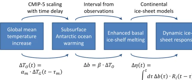
Here we use linear response theory to project ice discharge for varying basal melt scenarios. The framework of linear re-sponse theory has been used before, for example to gener-alize climatic response to greenhouse gas emissions (Good et al., 2011). The probabilistic procedure for obtaining pro-jections of the Antarctic dynamic discharge due to basal ice-shelf melt and its uncertainty range is described in Sect. 4 and illustrated in Fig. 1. There are clear limitations to this approach which are discussed in the conclusions section at the end. In light of these limitations, which range from the use of linear response theory to missing physical process in the ice sheet but also in the oceanic models, the results pre-sented here need to be considered as a first approach towards an estimate of Antarctica’s future dynamic contribution to sea-level rise.

2 Brief description of the ice-sheet and ocean models

(3)

Global mean temperature increase

Subsurface Antarctic ocean

warming

Enhanced basal

ice‐shelf melting

Dynamic ice‐

sheet response CMIP‐5 scaling

with time delay

Interval from observations

Continental ice‐sheet models

∆

∙ ∆ ∆ ∙ ∆ ∆

∆ ∙

Figure 1. Schematic of procedure for the estimate of the uncertainty of the Antarctic dynamic contribution to future sea-level change. At each stage of the procedure, represented by the four boxes, a random selection is performed from a uniform distribution as indicated in the following. This procedure was carried out 50 000 times for each RCP scenario to obtain the uncertainty ranges described throughout the study. First, one time evolution of the global mean temperature,1TG, was selected randomly out of an ensemble of 600 MAGICC-6.0 simulations. Second, 1 of 19 CMIP-5 climate models was selected randomly to obtain the scaling coefficient and time delay between the global mean temperature surface warming,1TG, and the subsurface oceanic warming,1TO. Third, a basal melt sensitivity,β, was selected randomly from the observed interval to translate the oceanic warming into additional basal ice-shelf melting. Finally, one of the ice-sheet models is selected randomly to use the corresponding response function,Ri, to obtain an ice discharge signal which is given in sea-level equivalent. The formulas describe the corresponding signal transformation at each step.

2013). Furthermore, the basal-melt sensitivity experiments which were used to derive the response function (as detailed in Sect. 3 were started from an equilibrium simulation and might thereby be biased towards a delayed response com-pared to the real Antarctic ice sheet which has evolved from a glacial period about 10 000 years ago.

AIF: the Anisotropic Ice-Flow model is a 3-D ice-sheet model incorporating anisotropic ice flow and fully coupling dynamics and thermodynamics (Wang et al., 2012). It is a higher-order model with longitudinal and vertical shear stresses but currently without an explicit representation of ice shelves. The model uses the finite difference method to calculate ice-sheet geometry including isostatic bedrock ad-justment, 3-D distributions of shear and longitudinal strain rates, enhancement factors which account for the effect of ice anisotropy, temperatures, horizontal and vertical veloci-ties, shear and longitudinal stresses. The basal sliding is de-termined by Weertman’s sliding law based on a cubic power relation of the basal shear stress. As the model lacks ice shelves, the prescribed melt rates are applied to the ice-sheet perimeter grid points whenever the bed is below sea level. The ice-sheet margin, which is equivalent to the grounding line in this model, moves freely within the model grid points and the grounding line is detected by hydrostatic equilibrium (i.e. the floating condition) without sub-grid interpolation.

PennState-3D: the Pennsylvania State University 3-D ice-sheet model uses a hybrid combination of the scaled shal-low ice approximation (SIA) and shalshal-low shelf approxima-tion (SSA) equaapproxima-tions for shearing and longitudinal stretch-ing flow respectively. The location of the groundstretch-ing line is determined by simple flotation, with sub-grid interpola-tion as in Gladstone et al. (2010). A parameterizainterpola-tion

re-lating ice velocity across the grounding line to local ice thickness is imposed as an internal boundary-layer condi-tion, so that grounding-line migration is simulated reason-ably well without the need for very high, i.e of the order of 100 m, resolution (Schoof, 2007). Ocean melting below ice shelves and ice-shelf calving use simple parameteriza-tions, along with a sub-grid parameterization at the floating-ice edge (Pollard and Deconto, 2009; Pollard and DeConto, 2012). The PennState-3D model shows the best performance of grounding line motion within the MISMIP intercompari-son compared to the other models applied here.

(4)

accounted for. The PISM model shows good performance of the grounding line motion within the MISMIP intercompar-isons only at significantly higher resolution (1 km or finer) than applied here.

SICOPOLIS: the SImulation COde for POLythermal Ice Sheets is a three-dimensional, polythermal ice-sheet model that was originally created by Greve (1995, 1997) in a version for the Greenland ice sheet, and has been devel-oped continuously since then (Sato and Greve, 2012) (www. sicopolis.net). It is based on finite-difference solutions of the shallow ice approximation for grounded ice (Hutter, 1983; Morland, 1984) and the shallow shelf approximation for floating ice (Morland, 1987; MacAyeal, 1989). Special at-tention is paid to basal temperate layers (that is, regions with a temperature at the pressure melting point), which are po-sitioned by fulfilling a Stefan-type jump condition at the in-terface to the cold ice regions. Basal sliding is parameter-ized by a Weertman-type sliding law with sub-melt sliding (which allows for a gradual onset of sliding as the basal temperature approaches the pressure melting point (Greve, 2005)), and glacial isostasy is described by the elastic litho-sphere/relaxing asthenosphere (ELRA) approach (Le Meur and Huybrechts, 1996). The position and evolution of the grounding line is determined by the floating condition. Be-tween neighbouring grounded and floating grid points, the ice thickness is interpolated linearly, and the half-integer aux-iliary grid point in between (on which the horizontal ve-locity is defined, Arakawa C grid) is considered as either grounded or floating depending on whether the interpolated thickness leads to a positive thickness above floatation or not. SICOPOLIS was not part of the MISMIP experiments (Pat-tyn et al., 2012). The performance of the ice-shelf solver was tested against the analytical solution for an ice-shelf ramp (Greve and Blatter, 2009, Sect. 6.4) and showed very good agreement of the horizontal velocity field already at low res-olution, as discussed by Sato (2012). The grounding line motion of the model has however not been systematically tested yet.

UMISM: the University of Maine Ice Sheet Model con-sists of a time-dependent finite-element solution of the cou-pled mass, momentum and energy conservation equations using the SIA (Fastook, 1990, 1993; Fastook and Chap-man, 1989; Fastook and Hughes, 1990; Fastook and Prentice, 1994) with a broad range of applications (for example, Fas-took et al., 2012, 2011) The 3-D temperature field, on which the flow law ice hardness depends, is obtained from a 1-D finite-element solution of the energy conservation equation at each node without direct representation of horizontal heat advection. This thermodynamic calculation includes verti-cal diffusion and advection, but neglects horizontal move-ment of heat. Also included is internal heat generation pro-duced by shear with depth and sliding at the bed. Bound-ary conditions consist of specified surface temperature and basal geothermal gradient. If the calculated basal tempera-ture exceeds the pressure melting point, the basal boundary

EAIS

Ross Sea Amundsen

Sea

Weddell Sea

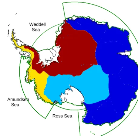
Figure 2. The four different basins for which ice-sheet response functions are derived from the SeaRISE M2 experiments. Green lines enclose the oceanic regions over which the subsurface oceanic temperatures were averaged. Vertical averaging was carried out over a 100 m depth range centred at the mean depth of the ice shelves in the region taken from Le Brocq et al. (2010) as provided in Table 1.

condition is changed to a specified temperature, and a basal melt rate is calculated from the amount of latent heat of fu-sion that must be absorbed to maintain this specified temper-ature. Conversely, if the basal temperature drops below the pressure melting point where water is already present at the bed, a similar treatment allows for the calculation of a rate of basal freezing. A map-plane solution for conservation of water at the bed, whose source is the basal melt or freeze-on rate provided by the temperature solution, allows for move-ment of the basal water down the hydrostatic pressure gra-dient (Johnson and Fastook, 2002). Areas of basal sliding can be specified if known, or determined internally by the model as regions where lubricating basal water is present, produced either by melting in the thermodynamic calcula-tion or by movement of water beneath the ice sheet down the hydrostatic gradient. Ice shelves are not modelled explicitly in UMISM. However, a thinning rate at the grounding line produced by longitudinal stresses is calculated from a pa-rameterization of the thinning of a floating slab (Weertman, 1957). No sub-grid grounding line interpolation is applied.

(5)

were used. These models typically apply an oceanic resolu-tion of several degrees both in latitude and longitude. This re-sults in the fact that major climate variability processes such as the El Niño–Southern Oscillation (ENSO) phenomenon are not accurately represented. Important for the results dis-cussed here is that these models are most likely not able to accurately represent the effects of mesoscale eddy motion. As shown, for example, by Hellmer et al. (2012) these might be crucial for abrupt warming events which may have signif-icant impact on basal ice-shelf melt. This is a major limita-tion of the results presented here. The models used are likely missing any abrupt warming and are only able to capture large-scale warming signals.

Besides the probabilistic projections we apply the ice-sheet response functions to subsurface temperature projec-tions from two different ocean models, namely the Bremer-haven Regional Ice Ocean Simulations (BRIOS) model and the Finite-Element Southern Ocean Model (FESOM).

BRIOS is a coupled ice–ocean model which resolves the Southern Ocean south of 50◦S zonally at 1.5◦ and merid-ionally at 1.5◦×cosφ. The water column is variably divided into 24 terrain-following layers. The sea-ice component is a dynamic–thermodynamic snow/ice model with heat budgets for the upper and lower surface layers (Parkinson and Wash-ington, 1979) and a viscous–plastic rheology (Hibler, 1979). BRIOS considers the ocean–ice-shelf interaction underneath 10 Antarctic ice shelves (Beckmann et al., 1999; Hellmer, 2004) with time-invariant thicknesses, assuming flux diver-gence and mass balance to be in dynamical equilibrium. The model has been successfully validated by the comparison with mooring and buoy observations regarding, e.g. Wed-dell gyre transport (Beckmann et al., 1999), sea ice thick-ness distribution and drift in Weddell and Amundsen seas (Timmermann et al., 2002a; Assmann et al., 2005) and sub-ice-shelf circulation (Timmermann et al., 2002b).

FESOM is a hydrostatic, primitive-equation ocean model with an unstructured grid that consists of triangles at the sur-face and tetrahedra in the ocean interior. It is based on the finite element model of the North Atlantic (Danilov et al., 2004, 2005) coupled to a dynamic–thermodynamic sea-ice model with a viscous–plastic rheology and evaluated in a global setup (Timmermann et al., 2009; Sidorenko et al., 2011). An ice-shelf component with a three-equation sys-tem for the computation of sys-temperature and salinity in the boundary layer between ice and ocean and the melt rate at the ice-shelf base (Hellmer et al., 1998) has been implemented. Turbulent fluxes of heat and salt are computed with coeffi-cients depending on the friction velocity following Holland and Jenkins (1999). The present setup uses a hybrid vertical coordinate and a global mesh with a horizontal resolution be-tween 30 and 40 km in the offshore Southern Ocean, which is refined to 10 km along the Antarctic coast, 7 km under the larger ice shelves in the Ross and Weddell seas and to 4 km under the small ice shelves in the Amundsen Sea.

Table 1.Mean depth of ice shelves in the different regions denoted in Fig. 2 as computed from Le Brocq et al. (2010). Oceanic temper-ature anomalies were averaged vertically over a 100 m range around these depth.

Region Depth [m]

Amundsen Sea 305

Ross Sea 312

Weddell Sea 420 East Antarctica 369

Outside the Southern Ocean, resolution decreases to 50 km along the coasts and to about 250–300 km in the vast basins of the Atlantic and Pacific oceans, while on the other hand, some of the narrow straits that are important to the global thermohaline circulation (e.g. Fram and Denmark straits, and the region between Iceland and Scotland) are represented with high resolution (Timmermann et al., 2012). Ice-shelf draft, cavity geometry, and global ocean bathymetry have been derived from the RTopo-1 data set (Timmermann et al., 2010) and thus consider data from many of the most recent surveys of the Antarctic continental shelf.

3 Deriving the response functions

In order to use the sensitivity experiments carried out within the SeaRISE project (Bindschadler et al., 2013), we assume that for the 21st century the temporal evolution of the ice discharge can be expressed as

S(t )=

t Z

0

dτ R (t−τ ) m (τ ) , (1)

whereS is the sea-level contribution from ice discharge,m is the forcing represented by the basal-melt rate andRis the ice-sheet response function.t is time starting from a period prior to the beginning of a significant forcing. The response functionRcan thus be understood as the response to a delta-peak forcing with magnitude one.

Sδ(t )= t Z

0

dτ R (t−τ ) δ (τ )=R (t )

(6)

0 2 4 6

x 10−4

R

Amundsen Sea

AIF PennState3D PISM SICOPOLIS UMISM

Ross Sea

0 25 50 75 100

0 2 4 6

x 10−4

Time (years)

R

Weddell Sea

0 25 50 75 100

Time (years) EAIS

AIF PennState3D PISM SICOPOLIS UMISM 1

3

1

0 Time (years) 500 x10−4

3

1

3

1

3

1

Figure 3. Linear response functions for the five ice-sheet models of Antarctica for each region as defined by Eq. (2) and as obtained from the SeaRISE-M2 experiments. The projections up to the year 2100, as computed here, will be dominated by the response functions up to year 100 since this is the period of the dominant forcing. For completeness, the inlay shows the response function for the full 500 years, i.e the period of the original SeaRISE experiments. As can be seen from Eq. (1), the response function is dimensionless. While the response functions are different for each individual basin and model when derived from the weaker M1 experiment (Fig. 14), the uncertainty range for the sea-level contribution in 2100 is very similar, since it is dominated by the uncertainty in the climatic forcing (compare Fig. 11).

Linear response theory, as represented by Eq. (1), can only describe the response of a system up to a certain point in time; 100 years is a relatively short period for the response of an ice sheet and the assumption of a linear response is thereby justified. During this period of validity, Eq. (1) is also capable of capturing rather complex responses such as irreg-ular oscillations (compare Fig. 3); the method is not restricted to monotonous behaviour. However, Eq. (1) implies that mul-tiplying the forcing by any factor will change the response by the same factor. This can only be the case as long as there are no qualitative changes in the physical response of the system. Furthermore, any self-amplifying process such as the marine ice-sheet instability will not be captured accurately by Eq. (1) if the process dominates the response. Linear response the-ory can still be a valid approach in this case if the forcing dominates the response of the system. The weak forcing lim-itation is particularly relevant for the low emission scenario RCP-2.6. The forcing is likely to dominate the response for the relatively strong SeaRISE experiment M2 with additional

homogeneous basal ice-shelf melting of 20 m a−1and for the strong warming scenario RCP-8.5 which is particularly rel-evant for an estimate of the full range of ice-discharge pro-jections. In this study, we project only for 100 years with a time-delayed oceanic forcing of several decades (as detailed in Tables 2–5) for the full coast line of Antarctica. For this particular setup, the linear response approach will provide insights into the continental response of the ice sheet.

(7)

0 1 2

Amundsen Sea

RCP−2.6 RCP−4.5 RCP−6.0

RCP−8.5 ₀

1 2

0 1 2

Ross Sea

RCP−2.6 RCP−4.5 RCP−6.0

RCP−8.5 ₀

1 2

0 1 2

Weddell Sea

RCP−2.6 RCP−4.5 RCP−6.0 RCP−8.5

Subsurface temperature anomaly (K) ₀

1 2

1900 2000 2100

0 1 2

East Antarctica

RCP−2.6 RCP−4.5 RCP−6.0 RCP−8.5

Year

0 1 2 0

1 2

0 1 2

0 1 2 0 1 2 0 1 2 2100

2100

1900

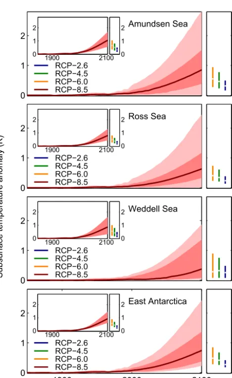
Figure 4. Oceanic subsurface-temperature anomalies outside the ice-shelf cavities as obtained from scaling the range of global mean temperature changes under the different RCP scenarios to the oceanic subsurface outside the ice-shelf cavities. For the downscal-ing, the oceanic temperatures were diagnosed off the shore of the ice-shelf cavities within the four regions defined in Fig. 2 at the depth of the mean ice-shelf thickness as defined in Table 1. These temperature anomalies were plotted against the global mean tem-perature increase for each of the 19 CMIP-5 climate models used here. The best scaling was obtained when using a time delay be-tween global mean temperature and oceanic subsurface temperature anomalies. The scaling coefficients with the respective time delay are provided in Tables 2–5. The thick red line corresponds to the median temperature evolution. The dark shading corresponds to the 66 % percentile around the median (red). The light shading corre-sponds to the 90 % percentile. Inlays show the temperature anoma-lies without time delay.

Table 2.Amundsen Sea sector: scaling coefficients and time delay

1tbetween increases in global mean temperature and subsurface ocean temperature anomalies.

Model Coeff. r2 1t Coeff. r2

without1t [yr] with1t

ACCESS1-0 0.17 0.86 0 0.17 0.86

ACCESS1-3 0.30 0.94 0 0.30 0.94

BNU-ESM 0.37 0.88 30 0.56 0.92

CanESM2 0.15 0.83 30 0.24 0.88

CCSM4 0.22 0.89 0 0.22 0.89

CESM1-BGC 0.19 0.92 0 0.19 0.92

CESM1-CAM5 0.12 0.92 0 0.12 0.92

CSIRO-Mk3-6-0 0.16 0.79 30 0.28 0.83

FGOALS-s2 0.24 0.90 55 0.54 0.93

GFDL-CM3 0.26 0.81 35 0.49 0.85

HadGEM2-ES 0.23 0.70 0 0.23 0.70

INMCM4 0.67 0.90 0 0.67 0.90

IPSL-CM5A-MR 0.07 0.22 90 0.44 0.45

MIROC-ESM-CHEM 0.12 0.74 5 0.13 0.75

MIROC-ESM 0.11 0.55 60 0.35 0.61

MPI-ESM-LR 0.27 0.80 5 0.29 0.82

MRI-CGCM3 0.00 0.02 85 -0.07 0.04

NorESM1-M 0.30 0.94 0 0.30 0.94

NorESM1-ME 0.31 0.89 0 0.31 0.89

Table 3.Weddell Sea sector: scaling coefficients and time delay1t

between increases in global mean temperature and subsurface ocean temperature anomalies.

ACCESS1-0 0.07 0.73 35 0.14 0.80

ACCESS1-3 0.07 0.73 35 0.15 0.81

BNU-ESM 0.37 0.89 0 0.37 0.89

CanESM2 0.11 0.82 55 0.31 0.91

CCSM4 0.37 0.95 20 0.49 0.96

CESM1-BGC 0.37 0.95 25 0.53 0.96

CESM1-CAM5 0.23 0.79 50 0.63 0.88

CSIRO-Mk3-6-0 0.19 0.80 55 0.60 0.90

FGOALS-s2 0.09 0.73 85 0.39 0.86

GFDL-CM3 0.11 0.55 60 0.31 0.62

HadGEM2-ES 0.31 0.92 0 0.31 0.92

INMCM4 0.26 0.83 10 0.30 0.83

IPSL-CM5A-MR -0.02 0.00 85 -0.06 0.03 MIROC-ESM-CHEM 0.07 0.50 65 0.32 0.77

MIROC-ESM 0.03 0.27 65 0.18 0.59

MPI-ESM-LR 0.08 0.65 85 0.41 0.70

MRI-CGCM3 0.21 0.63 40 0.47 0.83

NorESM1-M 0.26 0.90 5 0.28 0.92

NorESM1-ME 0.25 0.85 50 0.64 0.92

(8)

Table 4.Ross Sea sector: scaling coefficients and time delay1t

between increases in global mean temperature and subsurface ocean temperature anomalies.

ACCESS1-0 0.18 0.77 20 0.26 0.79

ACCESS1-3 0.09 0.76 15 0.12 0.77

BNU-ESM 0.28 0.83 20 0.36 0.84

CanESM2 0.14 0.74 45 0.32 0.80

CCSM4 0.14 0.91 5 0.15 0.92

CESM1-BGC 0.14 0.90 0 0.14 0.90

CESM1-CAM5 0.16 0.85 0 0.16 0.85

CSIRO-Mk3-6-0 −0.06 0.28 0 −0.06 0.28

FGOALS-s2 0.18 0.89 60 0.45 0.93

GFDL-CM3 0.23 0.85 25 0.37 0.89

HadGEM2-ES 0.25 0.62 0 0.25 0.62

INMCM4 0.59 0.83 0 0.59 0.83

IPSL-CM5A-MR 0.02 0.04 95 0.14 0.12

MIROC-ESM-CHEM 0.23 0.85 0 0.23 0.85

MIROC-ESM 0.23 0.78 0 0.23 0.78

MPI-ESM-LR 0.16 0.70 40 0.31 0.73

MRI-CGCM3 0.08 0.04 0 0.08 0.04

NorESM1-M 0.12 0.79 0 0.12 0.79

NorESM1-ME 0.12 0.68 20 0.16 0.73

Table 5. East Antarctic Sea sector: scaling coefficients and time delay1t between increases in global mean temperature and sub-surface ocean temperature anomalies.

ACCESS1-0 0.20 0.92 30 0.35 0.94

ACCESS1-3 0.27 0.92 0 0.27 0.92

BNU-ESM 0.35 0.92 0 0.35 0.92

CanESM2 0.21 0.96 0 0.21 0.96

CCSM4 0.13 0.96 5 0.13 0.97

CESM1-BGC 0.12 0.94 25 0.17 0.95

CESM1-CAM5 0.15 0.94 0 0.15 0.94

CSIRO-Mk3-6-0 0.22 0.93 15 0.28 0.94

FGOALS-s2 0.17 0.90 55 0.41 0.94

GFDL-CM3 0.21 0.89 35 0.39 0.93

HadGEM2-ES 0.23 0.95 0 0.23 0.95

INMCM4 0.55 0.97 0 0.55 0.97

IPSL-CM5A-MR 0.14 0.89 0 0.14 0.89

MIROC-ESM-CHEM 0.11 0.89 0 0.11 0.89

MIROC-ESM 0.09 0.85 50 0.24 0.88

MPI-ESM-LR 0.20 0.94 15 0.26 0.95

MRI-CGCM3 0.26 0.94 0 0.26 0.94

NorESM1-M 0.15 0.76 0 0.15 0.76

NorESM1-ME 0.15 0.74 60 0.49 0.85

integral of the response functionRwitht=0 being the time of the switch-on in forcing:

Ssf(t )=

t Z

0

dτ R (t−τ ) 1m0·2 (τ )=1m0·

t Z

0

dτ R (τ ) ,

where2 (τ )is the Heaviside function which is zero for neg-ativeτand one otherwise. We thus obtain the response

func-Table 6.Projections of ice discharge in 2100 according to Fig. 12. Numbers are in metres sea-level equivalent for the different global climate RCP scenarios with and without time delay1t. The models PennState-3D, PISM and SICOPOLIS have an explicit representa-tion of ice-shelf dynamics and are denoted “shelf models”.

Setup RCP Median 17 % 83 % 5 % 95 %

Shelf models 2.6 0.07 0.02 0.14 0.0 0.23 with1t 4.5 0.07 0.03 0.16 0.01 0.27 6.0 0.07 0.03 0.17 0.01 0.28 8.5 0.09 0.04 0.21 0.01 0.37

Shelf models 2.6 0.09 0.04 0.17 0.02 0.25 without1t 4.5 0.11 0.05 0.20 0.02 0.30 6.0 0.11 0.05 0.21 0.02 0.31 8.5 0.15 0.07 0.28 0.04 0.43

All models 2.6 0.08 0.03 0.17 0.01 0.27 with1t 4.5 0.09 0.03 0.20 0.01 0.33 6.0 0.09 0.03 0.20 0.01 0.34 8.5 0.11 0.04 0.27 0.01 0.47

All models 2.6 0.11 0.05 0.19 0.02 0.29 without1t 4.5 0.13 0.06 0.24 0.03 0.36 6.0 0.13 0.06 0.25 0.03 0.38 8.5 0.18 0.08 0.34 0.04 0.54

tion from

R (t )= 1 1m0

·dSsf

dt (t ). (2)

(9)

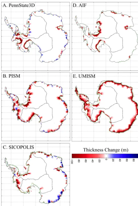
Figure 5. Ice-thickness change after 100 years under the SeaRISE experiment with homogeneous increase in basal ice-shelf melting of 20 m a−1(experiment M2 and Fig. 8 in Nowicki et al., 2013a). Due to their coarse resolution, some models with explicit represen-tation of ice shelves such as the PISM model tend to underestimate the length of the coastline to which an ice shelf is attached which might lead to an underestimation of the ice loss. The UMISM model assumes basal melting along the entire coastline which is likely to result in an overestimation of the effect. Black contours represent the initial grounding line which moved to the green contour during the M2 experiment after 100 years. Lines within the continent show the drainage basins as in Fig. 2

The spatial distribution of the ice loss after 100 years through additional basal ice-shelf melting illustrates the dif-ferent dynamics of the ice-sheet models resulting from, for example, different representations of ice dynamics, surface mass balance, basal sliding parameterizations and numerical implementation (Fig. 5). Part of the individual responses re-sult from the different representations of the basal ice-shelf melt. In the UMISM model, basal melt was applied along the entire coastline which yields a particularly strong response in East Antarctica (Fig. 3). This is likely an overestimation of ice loss compared to models with an explicit representation

of ice shelves. On the other hand, coarse-resolution ice-sheet models as used here cannot capture small ice shelves as they are present especially around East Antarctica. These mod-els thus have a tendency to underestimate the fraction of the coastal ice that is afloat and thus the sensitivity to changes in ocean temperature might be also underestimated (com-pare, for example, Martin et al. (2011) for the PISM model). While we will also provide projections using all five models, the main focus of the study is on the three models with ex-plicit representation of ice shelves (PennState-3D, PISM and SICOPOLIS).

4 Probabilistic approach

We aim to estimate the sea-level contribution from Antarc-tic dynamic ice discharge induced by basal ice-shelf melting driven by the global mean temperature evolution. In order to capture the climate uncertainty as well as the uncertainty in the oceanic response and the ice-sheet response, we follow a probabilistic approach that comprises four steps.

The schematic in Fig. 1 illustrates the procedure. At each of the four stages, represented by the four boxes, a random selection is performed from a uniform distribution as indi-cated in the following. The equations for each step are pro-vided in Fig. 1.

a. For each scenario, a climate forcing, i.e. global mean temperature evolution, that is consistent with the ob-served climate change and the range of climate sensitiv-ity of 2–4.5◦C for a doubling of CO2is randomly and uniformly selected from an ensemble of 600 MAGICC-6.0 simulations. This selection yields a global mean temperature time series,1TG, from the year 1850 to the year 2100.

b. Second, 1 of 19 CMIP-5 climate models is selected ran-domly to obtain the scaling coefficient and time delay between the global mean temperature surface warm-ing, 1TG, and the subsurface oceanic warming, 1TO. The global mean temperature evolution from step (a) is translated into a time series of subsurface ocean temper-ature change by use of the corresponding scaling coef-ficients and the associated time delay.

c. Third, a basal melt sensitivity,β, is selected randomly from the observed interval, to translate the oceanic warming into additional basal ice-shelf melting. The coefficient to translate the subsurface ocean tempera-ture evolution into a sub-shelf melt rate is randomly drawn from the observation-based interval 7 m a−1K−1 (Jenkins, 1991) to 16 m a−1K−1(Payne et al., 2007).

(10)

combine them with random selections of the forcing ob-tained from steps (a)–(c).

The procedure is repeated 50 000 times for each RCP sce-nario.

4.1 Global mean temperature evolution

We here use the Representative Concentration Pathways (RCPs) (Moss et al., 2010; Meinshausen et al., 2011b). The range of possible changes in global mean temperature that result from each RCP is obtained by constraining the re-sponse of the emulator model MAGICC 6.0 (Meinshausen et al., 2011a) with the observed temperature record. This pro-cedure has been used in several studies and aims to cover the possible global climate response to specific greenhouse-gas emission pathways (e.g. Meinshausen et al., 2009). Here we use a set of 600 time series of global mean temperature from the year 1850 to 2100 for each RCP that cover the full range of future global temperature changes as detailed in Schewe et al. (2011).

4.2 Subsurface oceanic temperatures from CMIP-5

We use the simulations of the recent Coupled Model Inter-comparison Project (CMIP-5) and obtain a scaling relation-ship between the anomalies of the global mean temperature and the anomalies of the oceanic subsurface temperature for each model. This has been carried out for the CMIP-3 exper-iments by Winkelmann et al. (2012) and is repeated here for the more recent climate models of CMIP-5.

Our scaling approach is based on the assumption that anomalies of the ocean temperatures resulting from global warming scale with the respective anomalies in global mean temperature. This approach may not be valid for absolute val-ues. The assumption is consistent with the linear-response assumption underlying Eq. (1). We use oceanic temperatures from the subsurface at the mean depth of the ice-shelf under-side in each sector (Table 1) to capture the conditions at the entrance of the ice-shelf cavities.

The surface warming signal needs to be transported to depth; therefore, the best linear regression is found with a time delay between global mean surface air temperature and subsurface oceanic temperatures. Results are detailed in Sect. 6.1. For the probabilistic projections, the scaling coef-ficients are randomly drawn from the provided sets.

4.3 Empirical basal melt coefficients

We apply an empirical relation to transform ocean temper-ature anomalies to basal ice-shelf melt anomalies. Observa-tions suggest an interval of 7 m a−1K−1 (Jenkins, 1991) to 16 m a−1K−1(Payne et al., 2007). See Holland et al. (2008) for a detailed discussion and comparison to other observa-tions. The coefficient used for each projection is drawn ran-domly and uniformly from this interval. For comparison, if

the temperature change were to be transported undiluted into the cavity and through the turbulent mixed layer underneath the ice shelf, the simple formula

m=ρOcpOγT ρiLi

·δTO≈42 m

aK·δTO (3)

would lead to a much higher melt rate, where ρO= 1028 kg m−3_and_c

pO=3974 J kg

−1_K−1_{are the density and} heat capacity of ocean water. ρi=910 kg m−3 and Li= 3.35×105J kg−1_{are ice density and latent heat of ice melt} andγT =10−4as adopted from Hellmer and Olbers (1989).

4.4 Translating melt rates into sea-level-relevant ice loss

The response functions as derived in Sect. 3 allow translat-ing the melttranslat-ing anomalies into changes in dynamic ice dis-charge from the Antarctic ice sheet. By randomly selecting a response function from the derived set, we cover the uncer-tainty from the different model responses. The main analysis is based on the response functions from the ice-sheet models with explicit ice-shelf representation. This choice was made because the application of the basal ice-shelf melting signal was less well defined for the models without explicit repre-sentation of the ice shelves. As a consequence the melting in these models was applied directly at the coast of the ice sheet in the first grounded grid cell. The area of melting was selected as the entire coast line in the case of the UMISM model and along the current shelf regions in the AIF model. These models were thus not included in the general uncer-tainty analysis.

5 Application of ice-sheet response functions to projections from regional ocean models

We first illustrate the direct application of the response func-tion outside the probabilistic framework. We use melt rate projections from the high-resolution global finite-element FESOM and the regional ocean model BRIOS to derive the dynamic ice loss from the Weddell and Ross sea sectors.

(11)

0 0.02 0.04

Ross−Sea Sector

FES − E1 FES − A1B BRIO − E1 BRIO − A1B PennState−3D

0 0.02 0.04

Weddell−Sea Sector

PennState−3D FES − E1 FES − A1B BRIO − E1 BRIO − A1B

0 0.02

PISM FES − E1 FES − A1B BRIO − E1 BRIO − A1B

0 0.05 0.1

PISM FES − E1 FES − A1B BRIO − E1 BRIO − A1B

0 0.02

SICOPOLIS FES − E1 FES − A1B BRIO − E1 BRIO − A1B

0 0.02

SICOPOLIS FES − E1 FES − A1B BRIO − E1 BRIO − A1B

0 0.02

AIF

FES − E1 FES − A1B BRIO − E1 BRIO − A1B

Sea level contribution (m)

0 0.05 0.1

AIF

FES − E1 FES − A1B BRIO − E1 BRIO − A1B

2000 2050 2100

0 0.02

UMISM FES − E1 FES − A1B BRIO − E1 BRIO − A1B

Year

2000 2050 2100

0 0.02 0.04

UMISM FES − E1 FES − A1B BRIO − E1 BRIO − A1B

Year

Figure 6. Ice loss as obtained from forcing the five response functions (Fig. 3) with the basal melt rates from the high-resolution global finite-element model FESOM (FES) and the regional ocean model BRIOS (BRIO). The full lines represent simulations in which BRIOS and FESOM were forced with the global climate model ECHAM-5; dashed lines correspond to a forcing with the HadCM-3 global climate model. Results are shown for the strong climate-change scenario A1B and the relatively low-emission scenario E1. A medium basal melt sensitivity of 11.5 m a−1K−1was applied. The results illustrate the important role of the global climatic forcing.

functions from the SeaRISE experiments are applicable in such a case.

Though ocean model and scenario uncertainty are present, Fig. 6 shows that the role of the global climate model in pro-jecting ice discharge is the dominating uncertainty as has al-ready been discussed by Timmermann and Hellmer (2013). It therefore encourages the use of the broadest possible spec-trum of climatic forcing in order to cover the high uncertainty from the choice of the global climate model.

6 Probabilistic projections of the Antarctic sea level contribution

6.1 Scaling coefficients for subsurface ocean temperatures

The scaling coefficients and the time delay determined from the 19 CMIP-5 coupled climate models are detailed in Ta-bles 2–5. The highr2values support the validity of the linear regression except for the IPSL model where also the slope between the two temperature signals is very low. We explic-itly keep this model in order to include the possibility that almost no warming occurs underneath the ice shelves.

(12)

0 10 20 0

500 1000

With time delay Without time delay

Counts

Sea level rise 1992−2011 (mm) 0

500 1000

PennState3D PISM SICOPOLIS with time delay

Counts

1900 1950 2000

0 10 20

With time delay Without time delay

Time (years)

Sea level rise (mm)

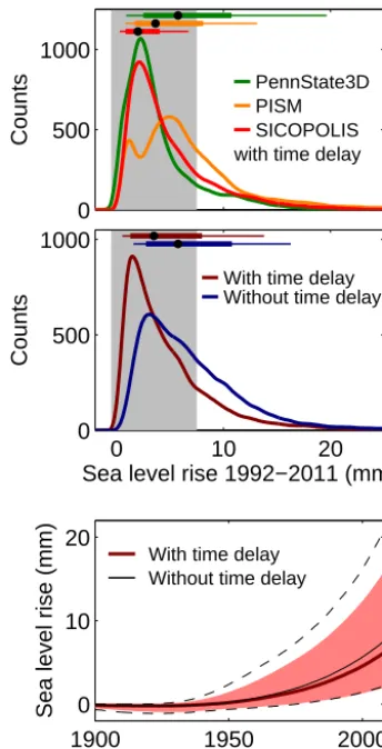
Figure 7. Uncertainty range including climate, ocean and ice-sheet uncertainty for the projected change of the observational period 1992–2011. Upper panel: probability distribution for the three mod-els with explicit representation of ice shelves (PennState-3D, PISM, SICOPOLIS). Middle panel: probability distribution with time de-lay (dark red) and without (dark blue) for three the models with explicit ice-shelf representation (shelf models). The grey shading in the upper two panels provides the estimated range from observa-tions following Shepherd et al. (2012). The likely range obtained with time delay is almost identical to the observed range. All dis-tributions are highly skewed towards high sea-level condis-tributions which strongly influences the median (black dot at the top of the panel), the 66 % range (thick horizontal line) and the 90 % range (thin horizontal line). Lower panel: time evolution for the hindcast projection using only the shelf models: with time delay, one obtains the red line as the median time series; the red shading provides the likely or 66 % range. The black line shows the median without time delay together with the likely range for this case as dashed lines.

scaling coefficient and the associated time delay1tfrom Ta-bles 2–5. Though physical reasons for a time delay between the surface and the subsurface temperatures exist, we find a high correlation also without applying a time delay. As the oceanic response of the coarse-resolution climate models ap-plied here is likely to underestimate some small-scale trans-port processes (i.e. Hellmer et al., 2012), it is useful to also

0 0.05 0.1

RCP−2.6 RCP−4.5 RCP−6.0 RCP−8.5

Amundsen Sea

0 0.05 0.1

RCP−2.6 RCP−4.5 RCP−6.0 RCP−8.5

Ross Sea

0 0.05 0.1

RCP−2.6 RCP−4.5 RCP−6.0 RCP−8.5

Weddell Sea

0 0.05 0.1

1900 2000 2100

0 0.05 0.1

RCP−2.6 RCP−4.5 RCP−6.0 RCP−8.5

East Antarctica

Year

0 0.05 0.1

Figure 8. Uncertainty range of contributions to global sea level from basal-melt induced ice discharge from Antarctica for the dif-ferent basins. Results shown here include the three ice-sheet models with explicit representation of ice-shelf dynamics and the global cli-mate forcing applied with a time delay as given in Tables 2–5. The full red curve is the median enclosed by the dark shaded 66 % range and the light shaded 90 % range of the distribution for the RCP-8.5 scenario. Coloured bars at the right show the other scenarios’ 66 % range intersected by the median. The full distribution is given in Fig. 9. The strongest difference between models with and without explicit representation of ice shelves occurs in East Antarctica as exemplified in the lower panel. The dashed black line envelopes the 66 % range of all models, the full black line is the median and the dotted line the 90 % percentile.

provide results without time delay to bracket the full range of response. The oceanic temperature time series without time delay are provided as inlays in Fig. 4.

(13)

0 1000 2000 3000

Amundsen Sea RCP−2.6 RCP−4.5 RCP−6.0 RCP−8.5

Counts

0 1000 2000 3000

Ross Sea RCP−2.6 RCP−4.5 RCP−6.0 RCP−8.5

Counts

0 1000 2000 3000

Weddell Sea RCP−2.6 RCP−4.5 RCP−6.0 RCP−8.5

Counts

0 0.05 0.1

0 1000 2000 3000

EAIS

RCP−2.6 RCP−4.5 RCP−6.0 RCP−8.5

Counts

Figure 9. Probability density function for the sea-level contribution from basal-melt-induced ice discharge for each region for the year 2100. Different colours represent the four RCP scenarios. Thick horizontal lines at the top of each panel provide the 66 % range of the distribution, the black dot is the median and the thin line the estimate of the 90 % range. Amundsen has the highest median contributions though sectors are relatively similar. Scenario depen-dency is strongest for the Amundsen region and East Antarctica. The distributions are highly skewed towards higher sea-level con-tributions. Results are shown for the models with explicit ice-shelf representation only.

Antarctica (25th to 75th percentiles of ensemble, West and East respectively) between 1951–2000 and 2091–2100.

6.2 Projected sea-level contribution for the past (1992–2011)

Figure 7 shows the uncertainty range of the sea-level projec-tion as obtained from this procedure for the sea-level change between 1992 and 2011 together with the range for this quan-tity as obtained from observations (Shepherd et al., 2012). The bars in the upper panels show that the likely range (66 % percentile) of the models with explicit ice-shelf representa-tions (PennState-3D, PISM and SICOPOLIS) are in good agreement with the observed range. The median (black dot) of each model is within the observed range. The middle panel shows that the time delay plays an important role. The likely range obtained from the models with explicit ice-shelf rep-resentation (denoted shelf models for simplicity) is almost identical to the observed range when the time delay is ac-counted for (dark red) while it reaches higher than the ob-served range without the time delay (dark blue). While we cannot claim that the ocean models or the ice-sheet models are capable of simulating the specific (and largely unknown) events that resulted in the sea-level contribution from Antarc-tica between 1992 and 2011, the observed signal corresponds well with our estimated range.

6.3 Results for the different basins and different models

Figure 8 shows the uncertainty range of the projected contri-bution from the different oceanic sectors comprising uncer-tainty in climate and ocean circulation. While the individual time series will differ from the non-probabilistic projections with the ocean models, FESOM and BRIOS, the order of magnitude of the range of the sea-level contribution is the same. For example, FESOM yields a particularly strong re-sponse in the Weddell sector when forced with the HadCM-3 model (dashed lines in Fig. 6) and BRIOS a weak response when forced with ECHAM-5. The response of the models from the downscaled global simulations covers this range. While we find the largest median response in the Amund-sen Sea sector which forces the Pine Island and Thwaites glaciers, the contributions of all sectors are relatively simi-lar with a scatter of the median from 0.01 to 0.03 m (Fig. 9). Note, however, that the contributions from the different re-gions are not independent and thus the median of the full ensemble cannot necessarily be obtained as the sum of the individual medians of the basins. The histogram of the ice-discharge contribution for the year 2100 in Fig. 9 shows the strongly skewed probability distribution.

(14)

0 0.2 0.4 RCP−2.6 RCP−4.5 RCP−6.0 RCP−8.5 PennState−3D 0 0.2 0.4 0 0.2 0.4 RCP−2.6 RCP−4.5 RCP−6.0 RCP−8.5 PISM 0 0.2 0.4 0 0.2 0.4 RCP−2.6 RCP−4.5 RCP−6.0 RCP−8.5 SICOPOLIS

Sea level contribution (m) 0

0.2 0.4 0 0.2 0.4 RCP−2.6 RCP−4.5 RCP−6.0 RCP−8.5 AIF Year 0 0.2 0.4

1900 2000 2100

0 0.2 0.4 RCP−2.6 RCP−4.5 RCP−6.0 RCP−8.5 UMISM Year 0 0.2 0.4

Figure 10. Uncertainty range of contributions to global sea level from basal-melt induced ice discharge from Antarctica for the dif-ferent ice-sheet models. Lines, shading and colour coding as in Fig. 8. Coloured bars at the right show the other scenarios’ 66 % range intersected by the median.

the base of our further analysis. The two models without ex-plicit ice-shelf dynamics, AIF and UMISM, however, yield responses of the same order of magnitude. The stronger re-sponse of the UMISM model is due to the fact that basal melt was applied along the entire coastline of Antarctica (Fig. 5), which is likely an overestimation of the real sit-uation. While there is a clear dependence on the climatic scenario especially for the 90 % percentile, the uncertainty between different ice-sheet models is comparable to the sce-nario spread. The strongest difference between models with and without explicit ice-shelf representation is observed in East Antarctica (dashed line in Fig. 8 provides the range for all models). The difference results mainly from the strong contribution of the UMISM model which assumes basal melt along the entire coastline.

0 0.1 0.2 0.3 0.4 0.5 RCP−2.6 RCP−4.5 RCP−6.0 RCP−8.5

All models with ∆ t

0 0.1 0.2 0.3 0.4 0.5

1900 2000 2100

0 0.1 0.2 0.3 0.4 0.5 RCP−2.6 RCP−4.5 RCP−6.0 RCP−8.5

All models without ∆ t

Year

0 0.1 0.2 0.3 0.4 0.5 0 0.1 0.2 0.3 0.4 0.5 RCP−2.6 RCP−4.5 RCP−6.0 RCP−8.5

Shelf models with ∆ t

0 0.1 0.2 0.3 0.4 0.5 0 0.1 0.2 0.3 0.4 0.5 RCP−2.6 RCP−4.5 RCP−6.0 RCP−8.5

Shelf models without ∆ t

0 0.1 0.2 0.3 0.4 0.5

Figure 11. Uncertainty range of contributions to global sea level from basal ice-shelf melt induced ice discharge from Antarctica including climate-, ocean- and ice-sheet model uncertainty. Lines, shading and colour coding as in Fig. 8. Estimates with and with-out the time delay between global mean surface air temperature and subsurface ocean temperature (Tables 2–5) are presented. Shelf models are those ice-sheet models with explicit representation of ice shelves.

6.4 Scenario dependence

(15)

the sea-level contribution is driven by the temperature in-crease in the atmosphere. Any natural variability in the at-mosphere, ocean or the ice sheet was not taken into ac-count. Given this methodological constraint, the scenario de-pendence is relatively small on these short timescales, espe-cially since it seems that on longer timescales the contribu-tion from Antarctica may depend significantly on the warm-ing level (e.g. Levermann et al., 2013). The results are sum-marized in Fig. 13. All distributions are significantly skewed towards high sea-level contributions. This skewness strongly influences the median of the distributions as well as the 66 and 90 % ranges. Consequently the median is not the value with the highest probability. The large tails makes an esti-mate of the 90 % range, i.e. the very likely range as denoted by the IPCC-AR5 (IPCC, 2013), very uncertain.

7 Conclusion and discussions

The aim of this study is to estimate the range of the potential sea-level contribution caused by future ice discharge from Antarctica that can be induced by ocean warming within the 21st century within the constraints of the models and the methodological approach. To this end, we include the full range of climatic forcing with climate models that yield prac-tically no warming of the Southern Ocean subsurface (e.g. IPSL) to extreme cases with more than 2◦C of warming at the entrance of the ice-shelf cavities under the strongest warming scenario (Fig. 4).

In constructing the method using linear response theory, the uncertainty ranges comprising climatic, oceanic and ice-dynamical uncertainty show a dependence on the global climate-change scenario (Table 6), especially for the tails of the distribution, e.g. the 95 % percentile. For the RCP-2.6 which was designed to result in a median increase in global mean temperature below 2◦C in most climate models, the 66 % range of ice loss is 0.02–0.14 m around a median of 0.07 m in units of global mean sea-level rise. This range in-creases to 0.04–0.21 m for RCP-8.5 with a median contribu-tion of 0.09 m. This compares to a likely range of−0.01 to 0.16 m for the dynamic Antarctic discharge until 2100 in the latest assessment report of the IPCC (Church et al., 2013). While the entire range was derived from a number of indi-vidual studies, the upper limit was mainly based on a proba-bilistic approach without specific accounting for the warming induced forcing Little et al. (2013a, b). This caused the limit to be independent of the scenario even though it was stated in the report that it is expected that the contribution will de-pend on the level of warming induced. It was further stated that this likely range can be exceed by several decimetres if the marine parts of the Antarctic ice sheet become unstable.

Our results are based on the three models with explicit rep-resentation of ice-shelf dynamics. The strongest difference to the ice-shelf models arises in the UMISM model which ap-plies melting along the entire coastline. For the main analysis

0

500 1000

1500

2000

RCP−8.5

Counts

0

500 1000

1500

2000

RCP−6.0

Counts

0

500 1000

1500

2000

RCP−4.5

Counts

0

0.2

0.4

0.6

0

500 1000

1500

2000

RCP−2.6

Sea level contribution (m)

Counts

Shelf models w ∆t Shelf models w\o ∆t All models w ∆t All models w\o ∆t

(16)

0 1000 2000

RCP−8.5 RCP−6.0 RCP−4.5 RCP−2.6 with time delay

Counts

0 0.2 0.4

0 1000 2000

RCP−8.5 RCP−6.0 RCP−4.5 RCP−2.6 without time delay

Counts

19000 2000 2100

0.1 0.2 0.3

0.4 _{With time delay} Without time delay

Time (years)

Sea level rise (m)

Figure 13. Uncertainty range including climate, ocean and ice-sheet uncertainty for the year 2100. Different colours represent dif-ferent scenarios using the three models including an explicit repre-sentation of ice shelves (PennState-3D, PISM, SICOPOLIS). The upper panel shows the results with time delay as listed in Tables 2– 5. The middle panel shows the results without this time delay. All distributions are highly skewed towards high sea-level contributions which strongly influences the median, the 66 % range (thick hori-zontal line at the top of the panel) and the 90 % range (thin horizon-tal line at the top of the panel). The scenario dependence is strongest in the higher percentile of the distribution as also visible in the num-bers provided in Table 6. The lower panel shows the corresponding time series of the median, the 66 % and the 90 % percentile of the distribution with and without time delay.

the models with explicit ice-shelf representation were se-lected for three main reasons: first, these models allowed a direct application of the central forcing, i.e. basal ice-shelf melting, without further parameterization of the effect of the basal ice-shelf melting on the ice flow. Second, these models capture the evolution of the ice-shelf area underneath which the melting takes place and third, the projected ice loss from Antarctica for the historic period of 1992 to 2011 agrees with observed contribution within the observational uncertainty.

It has to be noted that the ice-sheet models as well as the climate models used here are coarse in horizontal model res-olution. At this resolution the ice-sheet models are not able to simulate the benchmark behaviour of the MISMIP inter-comparison projects (Pattyn et al., 2012, 2013). Two of the models used (PennState-3D and PISM) are able to simulate the grounding line behaviour in accordance with analytic so-lutions or the full-Stokes solution in MISMIP when using a significantly higher resolution (around 1 km) than applied for the SeaRISE experiments (Pattyn et al., 2013; Feldmann et al., 2014). However, for continent-scale simulations, these high resolutions remain a challenge for ice-sheet models due to either the high computational costs or inadequate data sets, such as poorly known bedrock topography in the vicinity of grounding lines.

Furthermore, a number of physical processes that might be relevant for Antarctica’s future contribution are not in-cluded in these models. Here we name only a few, but this list is most likely not complete because modelling the effect of basal topography, surface melt and interaction between the ice-sheet-shelf system and the ocean is still far from suffi-cient. For example, the effect of ice calving from ice shelves, but potentially even more importantly, from ice sheets into the ocean (Bassis and Jacobs, 2013; Levermann et al., 2012; Bassis, 2011; Walter et al., 2010) is not properly represented in most models. The effect of changes in surface properties and resulting changes in basal lubrication or ice rheology are either not included or likely not sufficiently represented (e.g. Box et al., 2012; Borstad et al., 2012; Cathles et al., 2011). Feedbacks from the ice melt to ocean circulation and the sea ice as well as possible water intrusion and interaction with the sediment are generally not represented (e.g. Gomez et al., 2013; Muto et al., 2013; Macayeal et al., 2012; Walter et al., 2012; Gomez et al., 2010; Hattermann and Levermann, 2010; Howat et al., 2010). While the focus of this study is the role of the uncertainty in external forcing, the resolution-based deficiencies as well as the missing physical processes in the models need to be taken into account when interpreting the results.

(17)

0 2 4 6

x 10−4

R

Amundsen Sea

Ross Sea

0 25 50 75 100

0 2 4 6

x 10−4

Time (years)

R

Weddell Sea

0 25 50 75 100

Time (years) EAIS

0 500

1 3

Time (years)

1900 2000 2100

0 0.1 0.2 0.3 0.4 0.5

All models with ∆ t

Year

1900 2000 21000

0.1 0.2 0.3 0.4 0.5 Shelf models with ∆ t

Year

x10−4

0 500

1 3

Time (years) x10−4

0 500

1 3

0 500

1 3

Figure 14. Response functions as obtained from the M1 experiment of the SeaRISE intercomparison with an additional uniform basal ice-shelf melting of 2 m a−1. The upper four panels correspond to Fig. 3. The lower two panels show the uncertainty range in sea-level projections with the M1 response functions from above. The ranges obtained are very similar to the ranges obtained with the M2 response functions as shown in Fig. 11. While the response functions are very different for the M1 experiment compared to the M2 experiment, the projected ranges of sea-level rise are similar which is consistent with the fact that the uncertainty arises mainly from the uncertainty in the external forcing of the ice sheets.

consecutive, potentially self-accelerating grounding line re-treat which may be significant (Favier et al., 2014; Joughin et al., 2014; Rignot et al., 2014; Mengel and Levermann, 2014).

However, the largest uncertainty in the future sea-level contribution estimated in this study arises from the uncer-tainty in the external forcing and here in particular from the uncertainty in the physical climate system, not in the socio-economic pathways. This may arise due to the fact that only few ice-sheet models were applied compared to the large number of climate models and warming paths. Further stud-ies are needed to assess whether large ice-sheet uncertainty arises with higher-resolution ice-sheet models. The

(18)

Internal variability was not accounted for, neither in the at-mosphere nor in the ocean or ice-sheet models. This is due to the coarse resolution of the applied models and may sig-nificantly influence the contribution for the 21st century (e.g. Hellmer et al., 2012).

The linear response approach sets further limits to the in-terpretation of our results. A significant response time of the sea-level-relevant ice flow to basal ice-shelf melting will be multi-decadal or longer which justifies the use of a linear re-sponse function to represent the full non-linear dynamics. A clear shortcoming is, however, that the method is not capa-ble of capturing self-amplification processes within the ice. As a consequence an irreversible grounding line motion will be captured only when it is forced and not if it is merely triggered by the forcing and then self-amplifies. Thus, if the ice loss due to an instability is faster than due to the exter-nal forcing, then this additioexter-nal ice loss will not be captured properly by the linear response theory. It is hypothesized that this is particularly relevant for weak forcing scenarios in which an instability might be triggered but the directly forced ice loss is weak. It might be less relevant for strong forcing scenarios like the RCP-8.5 when the forcing might dominate the dynamics.

Changes in the geometry of the ice-shelf cavity and salin-ity changes due to meltwater cannot be accounted for in a systematic way here. While the three ice-sheet models with ice-shelf representation within the limitation of their res-olution incorporate dynamic shelf evres-olution, the geometry changes cannot feed back to the ocean circulation in our linear response approach. The computation of the basal ice-shelf melt anomalies from the temperature anomalies is sim-plified as it excludes salinity changes. However, the simpli-fication well approximates the dominating dynamics as the effect of salinity anomalies is small (Payne et al., 2007). To account for the feedbacks between ice thickness and salinity changes due to meltwater and the ocean circulation, interac-tive coupling of ice shelves models and global climate mod-els is needed. As dynamic ice-shelf modmod-els are not imple-mented in the CMIP-5 climate models applied, the feedbacks cannot be reliably projected within the probabilistic approach taken here. We do not account for melt patterns underneath the ice shelves as basal melt rates are applied uniformly. While it has been shown that the melting distribution mat-ters for the ice-sheet response (Walker et al., 2008; Gagliar-dini et al., 2010), it is beyond the scope of this study as a dynamic ocean model is not applied. The melt coefficients applied here were derived for an ice-shelf average and new uncertainty would be introduced with a spatially dependent melt coefficient.

As discussed above, a time lag between the oceanic tem-perature change and the change in global mean tempera-ture is physically reasonable and applied in our projections. However, the correlation between surface warming and sub-surface temperature change improves only marginally when introducing the time lag and it is not clear whether small-scale processes may accelerate the heat transport at finer resolution (Hellmer et al., 2012). It is thus worthwhile to consider the ice loss without a time lag (Fig. 11b). If the basal ice-shelf melt rates are applied immediately, the 66 % range of the sea-level contribution increases from 0.04–0.21 to 0.07–0.28 m for RCP-8.5. The simulations with the high-resolution finite-element ocean model FESOM and the re-gional ocean model BRIOS (Fig. 6) illustrate that abrupt ocean circulation changes can have strong influence on the basal melt rates (Hellmer et al., 2012). The comparably coarse-resolution ocean components of the CMIP-5 global climate models are unlikely to resolve such small-scale changes. Estimates such as those presented here will thus be dominated by basin-scale temperature changes of the interior ocean.

The probabilistic approach applied here assumes a certain interdependence of the different uncertainties. The global cli-matic signal is selected independently from the oceanic scal-ing coefficient. However, the range of scalscal-ing coefficients is derived from the correlation within the different CMIP-5 models. The ice-sheet uncertainty is again independent of the other two components. While there are other methods to combine the uncertainties, we find no clear way of judging which method is superior.

(19)

Appendix A: Linear response function derived from SeaRISE M1 experiment

Figure 14 shows the response functions as obtained from the M1 experiment with 2 m a−1of additional basal ice-shelf melting. Comparison with Fig. 3 shows significant differ-ences between the response functions obtained from the M1 and M2 experiments.

(20)

Acknowledgements. R. Winkelmann and M. A. Martin were funded by the German federal ministry of education and research (BMBF grant 01LP1171A). M. Meinshausen was funded by the Deutsche Bundesstiftung Umwelt. R. Greve and T. Sato were supported by a Grant-in-Aid for Scientific Research A (no. 22244058) from the Japan Society for the Promotion of Science (JSPS). S. Nowicki, R. A. Bindschadler, and W. L. Wang were supported by the NASA Cryospheric Science program (grants 281945.02.53.02.19 and 281945.02.53.02.20). K. Frieler was sup-ported by the German Federal Ministry for the Environment, Nature Conservation and Nuclear Safety (11_II_093_Global_A_SIDS and LDCs). H. H. Hellmer, A. J. Payne and R. Timmermann were supported by the ice2sea programme from the European Union 7th Framework Programme, grant no. 226375.

Edited by: M. Huber

References

Albrecht, T., Martin, M. A., Winkelmann, R., Haseloff, M., and Levermann, A.: Parameterization for subgrid-scale mo-tion of ice-shelf calving fronts, The Cryosphere, 5, 35–44, doi:10.5194/tc-5-35-2011, 2011.

Alley, R., Berntsen, T., Bindoff, N. L., Chen, Z., Chidthaisong, A., Friedlingstein, P., Hegerl, G., Heimann, M., Hewitson, B., Hoskins, B., Joos, F., Jouzel, J., Kattsov, V., Lohmann, U., Man-ning, M., Matsuno, T., Molina, M., Nicholls, N., Overpeck, J., Qin, D., Ramaswamy, V., Ren, J., Rusticucci, M., Solomon, S., Somerville, R., Stocker, T. F., Stott, P., Stouffer, R. J., Whetton, P., Wood, R. A., Wratt, D., Arblaster, J., Brasseur, G., Chris-tensen, J. H., Denman, K., Fahey, D. W., Forster, P., Jansen, E., Jones, P. D., Knutti, R., Treut, H. L., Lemke, P., Meehl, G., Mote, P., Randall, D., Stone, D. A., Trenberth, E., Willebrand, J., and Zwiers, F.: Climate Change 2007: The Physical Science Basis. Contribution of Working Group I to the Fourth Assess-ment Report of the IntergovernAssess-mental Panel on Climate Change, Cambridge University Press, Cambridge, UK and New York, NY, USA, 2007.

Aschwanden, A., Bueler, E., Khroulev, C., and Blatter, H.: An en-thalpy formulation for glaciers and ice sheets, J. Glaciol., 58, 441–457, doi:10.3189/2012JoG11J088, 2012.

Assmann, K. M., Hellmer, H. H., and Jacobs, S. S.: Amundsen Sea ice production and transport, J. Geophys. Res., 110, 311–337, 2005.

Bamber, J. L., Riva, R. E. M., Vermeersen, B. L. A., and LeBrocq, A. M.: Reassessment of the Potential Sea-Level Rise from a Col-lapse of the West Antarctic Ice Sheet, Science, 324, 901–903, doi:10.1126/science.1169335, 2009.

Bassis, J. N.: The statistical physics of iceberg calving and the emer-gence of universal calving laws, J. Geol., 57, 3–16, 2011. Bassis, J. N. and Jacobs, S.: Diverse calving patterns linked to

glacier geometry, Nat. Geosci., 6, 1–4, doi:10.1038/ngeo1887, 2013.

Beckmann, A., Hellmer, H. H., and Timmermann, R.: A numeri-cal model of the Weddell Sea: Large-snumeri-cale circulation and water mass distribution, Geophys. Res. Lett., 104, 23375–23391, 1999.

Bindschadler, R. A., Nowicki, S., Abe-Ouchi, A., Aschwanden, A., Choi, H., Fastook, J., Granzow, G., Greve, R., Gutowski, G., Herzfeld, U., Jackson, C., Johnson, J., Khroulev, C., Levermann, A., Lipscomb, W. H., Martin, M. A., Morlighem, M., Parizek, B. R., Pollard, D., Price, S. F., Ren, D., Saito, F., Sato, T., Seddik, H., Seroussi, H., Takahashi, K., Walker, R., and Wang, W. L.: Ice-sheet model sensitivities to environmental forcing and their use in projecting future sea level (the SeaRISE project), J. Glaciol., 59, 195–224, doi:10.3189/2013JoG12J125, 2013.

Borstad, C. P., Khazendar, A., Larour, E., Morlighem, M., Rignot, E., Schodlok, M. P., and Seroussi, H.: A damage mechanics as-sessment of the Larsen B ice shelf prior to collapse: Toward a physically-based calving law, Geophys. Res. Lett., 39, L18502, doi:10.1029/2012GL053317, 2012.

Box, J. E., Fettweis, X., Stroeve, J. C., Tedesco, M., Hall, D. K., and Steffen, K.: Greenland ice sheet albedo feedback: thermo-dynamics and atmospheric drivers, The Cryosphere, 6, 821–839, doi:10.5194/tc-6-821-2012, 2012.

Bueler, E. and Brown, J.: The shallow shelf approximation as a sliding law in a thermomechanically coupled ice sheet model, J. Geophys. Res., 114, F03008, doi:10.1029/2008JF001179, 2009. Cathles, L. M., Abbot, D. S., Bassis, J. N., and MacAyeal, D. R.: Modeling surface-roughness/solar-ablation feedback: application to small-scale surface channels and crevasses of the Greenland ice sheet, Ann. Glaciol., 52, 99–108, doi:10.3189/172756411799096268, 2011.

Church, J., Clark, P., Cazenave, A., Gregory, J., Jevrejeva, S., Lever-mann, A., Merrifield, M., Milne, G., Nerem, R., Nunn, P., Payne, A., Pfeffer, W., Stammer, D., and Unnikrishnan, A.: Sea Level Change, in: Climate Change 2013: The Physical Science Basis. Contribution of Working Group I to the Fifth Assessment Re-port of the Intergovernmental Panel on Climate Change, Cam-bridge University Press, CamCam-bridge, UK and New York, NY, USA, 2013.

Danilov, S., Kivman, G., and Schröter, J.: A finite element ocean model: principles and evaluation, Ocean Modell., 6, 125–150, 2004.

Danilov, S., Kivman, G., and Schröter, J.: Evaluation of an eddy-permitting finite-element ocean model in the North Atlantic, Ocean Modell., 10, 35–49, 2005.

Fastook, J. L.: A map-plane finite-element program for ice sheet reconstruction: A steady-state calibration with Antarctica and a reconstruction of the Laurentide Ice Sheet for 18,000 BP, in: Computer Assisted Analysis and Modeling on the IBM 3090, edited by: Brown, H. U., IBM Scientific and Technical Comput-ing Dept., White Plains, N.Y., 1990.

Fastook, J. L.: The finite-element method for solving conservation equations in glaciology, Comput. Sci. Eng., 1, 55–67, 1993. Fastook, J. L. and Chapman, J.: A map plane finite-element model:

Three modeling experiments, J. Glaciol., 35, 48–52, 1989. Fastook, J. L. and Hughes, T. J.: Changing ice loads on the

Earth’s surface during the last glacial cycle, in: Glacial Isostasy, Sea-Level and Mantle Rheology, Series C: Mathematical and Physical Sciences, Vol. 334, edited by: Sabadini, R., Lam-beck, K., and Boschi, E., Kluwer Academic Publishers, Dor-drecht/Boston/London, 1990.