www.nonlin-processes-geophys.net/20/955/2013/ doi:10.5194/npg-20-955-2013
© Author(s) 2013. CC Attribution 3.0 License.
Nonlinear Processes
in Geophysics
Using ensemble data assimilation to forecast hydrological flumes
I. Amour, Z. Mussa, A. Bibov, and T. Kauranne
Lappeenranta University of Technology, Lappeenranta, Finland Correspondence to: I. Amour ([email protected])
Received: 29 May 2013 – Revised: 23 September 2013 – Accepted: 9 October 2013 – Published: 8 November 2013
Abstract. Data assimilation, commonly used in weather forecasting, means combining a mathematical forecast of a target dynamical system with simultaneous measurements from that system in an optimal fashion. We demonstrate the benefits obtainable from data assimilation with a dam break flume simulation in which a shallow-water equation model is complemented with wave meter measurements. Data as-similation is conducted with a Variational Ensemble Kalman Filter (VEnKF) algorithm. The resulting dynamical analysis of the flume displays turbulent behavior, features prominent hydraulic jumps and avoids many numerical artifacts present in a pure simulation.
1 Introduction
Hydrological flumes and other phenomena related to rivers, estuaries, canals, and other water bodies that lend themselves to a one- or two-dimensional description have received some-what less attention in computational fluid dynamics (CFD) research than flows in industrial processes, or fully three-dimensional flows in general. However, there is one notable exception, namely, weather forecasting.
Weather models are complex codes that have received a lot of attention from the CFD community since the 1950s. Many techniques employed in weather forecasting are natu-rally amenable to other hydrostatic flows, such as river, estu-ary, and canal flows, but have yet to be tried in these applica-tions. One of the most prominent of such techniques is data assimilation.
In the current paper, we introduce data assimilation of wave meter data into a river model that was originally pre-sented by Martin and Gorelick (2005). Data assimilation is a process that optimally combines model forecasts with ob-servations. In weather forecasting, data assimilation is used to generate the initial conditions for an ensuing forecast, but
also to continuously correct a forecast towards observations, whenever these are available in the course of the forecast.
Turbulence, which is an irregular motion found in fluids (liquids and gases) when passing objects or streamlines of itself passing one another (Goldstein, 1938), is the main rea-son that makes the CFD model ambitious to assimilate, as we hope for more information from the available measurements to shape the behavior of the model estimates.
In the paper of Martin and Gorelick (2005), the authors present a shallow-water model of a dam break experiment conducted in a laboratory. The goal of the model is to sim-ulate the behavior of the flume in the case that a dam sud-denly breaks. Results from numerical simulations are com-pared with measurements by wave meters and pressure trans-ducers that record water height during the experiment.
In the current article, we take the model and the measure-ments into account simultaneously in a process of continuous data assimilation. This results in a more realistic representa-tion of the behavior of the flume during the experiment, in the sense that the resulting flume displays turbulent behav-ior, features prominent hydraulic jumps and avoids many nu-merical artifacts present in a pure simulation. As our data as-similation algorithm, we have chosen a recent version of the Ensemble Kalman Filter, the Variational Ensemble Kalman Filter (VEnKF) introduced by Solonen et al. (2012). Ensem-ble Kalman filters have the distinct advantage over other data assimilation methods that they can be implemented as “wrap-pers” on top of existing CFD codes without necessitating modification of the models themselves. Moreover, they con-duct data assimilation continuously, so that their results can be compared with direct numerical simulations.
data assimilation and describes how it was implemented in the current research effort. Section five describes the dam break experiment and the way data assimilation was mod-ified to accommodate the model and the data in this case. Section six describes the results of numerical tests, both with and without data assimilation. Section seven concludes the paper.
2 Numerical simulation of river flows
Simulation of river flows presents challenges to computa-tional schemes due to the complex geometry and meander-ing path of the flow. Different schemes have been suggested and applied to try to capture as much information about the river as possible. A two-dimensional finite-element solution has been used to simulate an 11 km long reach of River Culm in Devon, UK, modeled by two-dimensional depth-averaged Reynolds equations (Bates and Anderson, 1993). The numer-ical model simulation finds an error of±2 % in continuity, although the mass conservation is still adequate.
The same method has been applied to flow simulations in Aliparast (2009). The governing equations of the model are 2-D shallow-water equations, where the stress term is ig-nored because of the influence of bottom roughness caused by turbulent shear stress between grids (Yoon and Kang, 2004). The numerical model has been validated by an exam-ple of an oblique hydraulic jump for which an analytical solu-tion is available (Aliparast, 2009). The numerical model has been tested with a dam break case in a converging-diverging flume (Bellos et al., 1991). The flume is 20.7 m long and 1.40 m wide, it has 5 stations used to record the water depth, and a dam is located 8.5 m from the closed end. The results of the dam break case simulation match well with the ex-perimental results (Aliparast, 2009). However, in station 4, which is 13.5 m downstream from the dam, water depth is underestimated.
The finite volume method is a further widely-used numer-ical scheme. It has been applied for a shallow water model in Heniche et al. (2000), Zhang and Wu (2011) and Ying et al. (2009).
A recent application on the dam break case is presented by Baghlani (2011), where a robust flux vector splitting (FVS) scheme is applied. FVS has been frequently applied in solving similar compressible flow problems (e.g. in Bagh-lani, 2011; Erpicum et al., 2010; Toro and Vazquez-Cendon, 2012). Two well-known FVS methods are that of Steger and Warming and that of Van Leer (Drikakis and Tsan-garis, 1993). Steger and Warming’s FVS exploits the ho-mogeneous property of the Euler equation and splits the fluxes into positive and negative parts with respect to the propagation (Drikakis and Tsangaris, 1993). Van Leer’s FVS constructs the fluxes as a function of the local Mach num-ber (Drikakis and Tsangaris, 1993). The FSV proposed by Baghlani (2011) decomposes the flux vector into positive and
negative components by means of Jacobian matrices of the flux vectors and a Liou–Steffen splitting for decomposing the pressure term. The FVS has been criticized for its expensive computational cost, as the eigensystem of equations must be evaluated at every time step (Baghlani, 2011).
One approach to studying flow behavior is to construct flume properties directly from measurements by regression. A method of surface analysis and velocity changes of this type has been presented (Barcena et al., 2012). It uses re-gression with respect to a collection of model scenarios to form a continuous function of hydrodynamic responses. The method has been successful in predicting estuarine free sur-face and velocity with significant savings in computational cost for a short- and medium-term simulation period. One advantage of this method is its ability to simulate a long-term hydrodynamic flow with a short computational time.
Pure 2-D simulations of hydrological flows suffer from several handicaps. Because the numerical flow is two-dimensional, it cannot capture the true three-dimensional flow, in particular turbulence: the numerical solution remains in perpetual hydrostatic balance. Even more importantly, the numerical time-stepping scheme implies that a flow front in front of a discontinuity, such as a flood wave, will only prop-agate one grid line per time step. The speed of this shock wave is therefore dependent on grid size and the numerical time step, and not on the correct physical speed. Finally, there is no way to connect the simulated flow to the true flow after the initial condition has been fixed. With data assimilation, we hope to address all three defects.
3 MODFreeSurf2D
MODFreeSurf2D is an open Matlab code that is designed to solve depth-averaged shallow-water equations (Martin and Gorelick, 2005). The code implements the semi-implicit, semi-Lagrangian time-stepping scheme of Casulli and Cheng (1992) and Casulli (1999), and uses a finite volume dis-cretization. The scheme is stable and can simulate water/land boundaries (Martin and Gorelick, 2005; Casulli and Cheng, 1992).
3.1 Depth-Averaged Shallow-Water Equations (DASWE)
The governing equations in MODFreeSurf2D are the depth-averaged shallow-water equations as given in Martin and Gorelick (2005):
∂U ∂t +U
∂U ∂x +V
∂U ∂y = −g
∂η ∂x+ε
∂2U
∂x2 + ∂2U
∂y2
+γT
(Ua−U )
H −g
√
U2+V2 C2
z
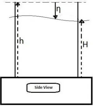
Fig. 1. ModFreeSurf2D variable definition (side view) which shows
the relationship between free surface elevationη, total water depth
H, and undisturbed water depthh(Martin and Gorelick, 2005).
∂V ∂t +U
∂V ∂x +V
∂V ∂y = −g
∂η ∂y+ε
∂2V
∂x2 + ∂2V
∂y2
+γT
(Va−V )
H −g
√
U2+V2 C2
z
V−f U, (2)
∂η ∂t +
∂(H U )
∂x +
∂(H V )
∂y =0, (3)
whereU is the depth-averagedx direction velocity compo-nent, V is the depth-averaged y direction velocity compo-nent, η is the free surface elevation, g is the gravitational constant,t is time,ε is the horizontal eddy viscosity,f is the Coriolis parameter,H=h+ηis the total water depth,
γT is the wind stress coefficient,Czis the Chezy coefficient,
andUa and Va are wind velocities. In the above,h is the
undisturbed water depth. Figure 1 illustrates the variable def-initions of MODFreeSurf2D.
Top friction and bottom friction boundaries are given by Eqs. (4) and (5), respectively.
ν∂U
∂z =γT(Ua−U ), ν ∂V
∂z =γT(Va−V ) (4)
ν∂U ∂z =g
√
U2+V2 C2
z
U, ν∂V ∂z =g
√
U2+V2 C2
z
V , (5)
whereν is the kinetic viscosity coefficient, andzindicates the vertical direction (Martin and Gorelick, 2005).
3.2 Numerical approximation
In MODFree2DSurf a combination of a implicit, semi-Lagrangian time-stepping scheme and a finite-volume dis-cretization is employed to numerically solve the hydrological shallow-water equations on a rectangular grid. This scheme
provides a stable solution, even for a time step larger than the Courant–Friedrichs–Lewy (CFL) restriction defined by CFL=w1t
1xi
, (6)
wherewis the velocity component in thexi direction,i=
1,2,1t is the time step size, and1xi is the cell dimension
in thexi direction of flow (Martin and Gorelick, 2005). The
CFL relates fluid velocity and time step size to computational cell size, and requires that it should be smaller than 1 (Martin and Gorelick, 2005).
3.2.1 Semi-implicit representation
In this representation, the free surface elevation η and the horizontal velocity componentsU andV are the unknown variables at timeN+1:
ηNi,j+1=ηNi,j−θ1t
1x H
N i+1/2,jU
N+1
i+1/2,j−H N i−1/2,jU
N+1
i−1/2,j
−θ1t
1x H
N i,j+1/2V
N+1
i,j+1/2−H
N i,j−1/2V
N+1
i,j−1/2
−(1−θ )1t
1x H
N i+1/2,jU
N
i+1/2,j−H N i−1/2,jU
N i−1/2,j
−(1−θ )1t
1x H
N
i,j+1/2Vi,jN+1/2−Hi,jN−1/2Vi,jN−1/2
,
(7)
UiN++1/12,j=F UiN+1/2,j−(1−θ )
g1t
1x η
N
i+1,j−ηi,jN
−θg1t
1x η
N+1
i+1,j−η N+1
i,j
+1tγT(Ua
−UiN++1/12,j)
HiN+1/2,j
−g1t q
(UiN+1/2,j)2+(VN i+1/2,j)2
Cz2i+1/2,jHiN+1/2,j U
N+1
i+1/2,j, (8)
Vi,jN++11/2=F Vi,jN+1/2−(1−θ )g1t
1y η
N
i,j+1−ηNi,j
−θg1t
1y η
N+1
i,j+1−η
N+1
i,j
+1tγT(Va
−Vi,jN++11/2)
Hi,jN+1/2
−g1t q
(Ui,jN+1/2)2+(VN i,j+1/2)2
Cz2i,j+1/2Hi,jN+1/2 V
N+1
i,j+1/2. (9)
The operatorsF U andF V in Eqs. (8) and (9) contain the advective, viscous, and Coriolis components of the govern-ing equations (Martin and Gorelick, 2005).
The value of the Chezy coefficient in Eq. (10) is given in terms of Manning’s roughness coefficientMn, which is assumed to be dimensionless (Martin and Gorelick, 2005). Other details of the discretization process can be found in Martin and Gorelick (2005):
Czi+1/2,j=
Hi+1/2,j1/6
Mni+1/2,j
. (10)
3.3 The boundary condition
The model itself identifies the location of water/land bound-aries using the following equations (Martin and Gorelick, 2005):
Hi+N+1/12,j=max 0, hi+1/2,j+ηi,jN+1, hi+1/2,j+ηN+i+11,j, (11)
Hi,j+N+11/2=max 0, hi,j+1/2+ηi,jN+1, hi,j+1/2+ηi,j+N+11. (12)
Two types of horizontal boundary conditions have been set:
(i) The projection of the velocity normal to the domain boundary:
∂U ∂t +Uupw
∂U
∂n =0, (13)
whereUupwis the upwinded normal direction velocity
com-ponent, andnis the direction normal to the domain boundary (Martin and Gorelick, 2005).
(ii) To limit wave reflections at open boundaries, the fol-lowing condition is imposed:
∂η ∂t +Cn
∂η
∂n=0, (14)
whereCnis the propagation velocity from grid points around
the boundary (Martin and Gorelick, 2005).
4 Data assimilation
4.1 Overview
Data assimilation aims to establish an optimal compromise between the prediction of a computational model and a set of observations. Both the model and the observations are as-sumed to be incorrect and contain some error. Heuristically, data assimilation takes some weighted average between these two estimates, with weights inversely proportional to the an-ticipated error in each (Daley, 1991).
Two forms of data assimilation have been common in weather forecasting. In “lumped” data assimilation, the goal is to produce a single initial state for the system to be simu-lated, from which a subsequent forecast can be launched. In
“lumped” data assimilation it has been possible to impose the model state equation – a set of conservation laws – exactly on that initial state, especially when so-called variational assim-ilation has been used (Le Dimet and Talagrand, 1986; Lewis and Derber, 1985; Courtier and Talagrand, 1987). However, variational data assimilation implicitly contains the same de-fects that the model it is based on contains – for example some model bias. Bias threatens to throw the model trajec-tory away from the true physical flow, which is tracked by observations even when they contain some noise.
In continuous data assimilation, on the other hand, the so-lution of the state equation is constantly “nudged” towards observations (Lorenc, 1986). This means that the state equa-tion is only approximately true and that several conservaequa-tion properties may get lost, but the model trajectory is likely to always stay close to the true observed trajectory.
The Extended Kalman Filter (EKF) (Kalman, 1960) com-bines the best properties of both lumped and continuous data assimilation methods. Unfortunately, the computational complexity of the classical EKF is prohibitively high for high-dimensional numerical models such as those appear-ing in geophysical simulations. However, this situation has started to change with the emergence of Ensemble Kalman filters (EnKF), (Evensen, 1994). Ensemble Kalman filters are stochastic approximations of the Extended Kalman Filter that purport to preserve many of its good properties. In practice, the degree to which this is achieved depends crucially on the particular EnKF variant chosen.
Some variants of Ensemble Kalman filters draw their in-spiration from the same Bayesian paradigm as the original Kalman Filter does. A prominent example of these methods is the maximum likelihood estimation filter (MLEF) intro-duced in Zupanski (2004). MLEF solves a Bayesian mini-mization with an ensemble of forecasts and uses the Limited Memory BFGS method to minimize a cost function that mea-sures the distance of observations from the forecast. How-ever, it generates a single ensemble of forecasts in the be-ginning of the forecast and uses it for all the minimzations, unlike the Variational Ensemble Kalman Filter (VEnKF) that will be introduced below. As will become evident from the convergence behavior of VEnKF, re-sampling the ensemble very frequently dramatically improves the convergence of the method and the stability of the corresponding Kalman filter.
4.2 VEnKF
The Variational Ensemble Kalman Filter (VEnKF) is a stochastic approximation of the EKF. In this paper, we re-strict ourselves to a brief discussion of the main ideas be-hind the VEnKF. A more detailed discussion can be found in Solonen et al. (2012). We begin by introducing the following coupled system of stochastic dynamic equations:
sk+1=Mk(sk)+εk, (15)
whereMk is anN-dimensional transition operator used to
forecast the model state at time instancek+1 given the model state at time instancek;Hk+1is an observation operator that
maps the model statesk+1 to the observationok+1;εk and
ζk+1are zero mean random terms that define prediction and
observation error, respectively. Our task is to define an esti-mate forsk+1given the operatorsMk,Hk+1, the observation ok+1, and the covariance matrices ofεk andζk+1, hereafter
defined asCεk andCζk+1. In many cases,εkandζk+1are also
assumed to be normally distributed, although this require-ment can be relaxed.
The motivation behind the VEnKF is quite similar to that of the EnKF. Foremost, we compute a sample estimate for the prior covariance, where the samples are explicitly generated by Eq. (15). Thereafter, instead of following the EKF formu-las as is done in EnKF, we replace them with a MAP (max-imum a posteriori probability) estimate problem. By taking
−log of the MAP cost function we arrive at an equivalent minimization problem as suggested in Auvinen et al. (2009):
l(s|ok+1)=
1 2 s−s
p
k+1
T
Ckp+1−1 s−skp+1+ (17) 1
2(ok+1−Hk+1(s))
TC−1
ζk+1(ok+1−Hk+1(s))).
Here skp+1 is the predicted model state at time instance
k+1 andCkp+1 is the covariance matrix of the prediction. When transition and observation operators are linear, it can be proven (Simon, 2006) that a minimum variance unbi-ased estimator forsk+1, hereafter denoted asskest+1, minimizes
Eq. (17), whereas the covariance matrix of this estimate, which we denote byCkest+1, is defined by the inverse Hessian of Eq. (17). This approach can also be expanded to non-linear cases.
Before giving a rigorous formulation of the VEnKF al-gorithm, we need to introduce some supporting notation. Let
ek,i Ni=1 denote an ensemble of cardinality N
sam-pled from the distribution ofskest. More precisely,∀i ek,i∼
N(sestk , Ckest). In addition, we denote the mean of ek,i Ni=1
bye¯kand introduce anM-element vectorX ek,idefined as
follows:
X ek,i
= ek,1− ¯ek
, . . . , ek,N− ¯ek
/
√ N−1.
The VEnKF algorithm now reads as follows:
i. Compute the model prediction:skp+1=Mk(sk).
ii. Move the ensembleek,i Ni=1forward using Eq. (15):
∀ie˜k+1,i=Mk ek,i.
iii. Define the sample estimate for the prior covariance:
Ckp+1=X e˜k+1,i
X e˜k+1,i
T
+Cεk.
iv. Assignskest+1to the minimizer of the cost function (17) andCkest+1 to an approximation of the inverse Hessian of Eq. (17).
v. Update the ensemble ˜ ek+1,i
N
i=1 by sampling from
N(skest+1, Ckest+1).
The strength of the VEnKF is that it allows a memory-efficient representation of the prior covarianceCkp+1. The lat-ter is advantageous when the model state dimension is too big to allow the explicit storage of the covariance matrices. How-ever, in order to implement steps (iv) and (v) of the presented algorithm, we need to evaluate the cost function defined by Eq. (17) and specify a low-memory approximation for its in-verse Hessian. The first goal is achieved by leveraging the Sherman–Morrison–Woodbury formula to invertCkp+1. More precisely:
Ckp+1−1=h
Cεk+X e˜k+1,i
X e˜k+1,i Ti−1
=Cε−1 k
−Cε−1
k X e˜k+1,i
I+ X e˜k+1,iTCε−k1X e˜k+1,i
−1
×
X e˜k+1,i
T
Cε−1
k . (18)
Formulation (18) can be directly inserted into cost func-tion (17), so it is not necessary to store the full matrices in order to evaluate it. Since the matrixCεk is usually specified
by a simplified (diagonal or block-diagonal) structure, and the ensemble size is assumed to be much smaller than the model state dimension, the inversion operations in Eq. (18) are feasible. Reverting back to the implementation of step (v) of the VEnKF algorithm, we suggest approximating the in-verse Hessian of Eq. (17) by either the full rank low-memory representation employed by the L-BFGS unconstraint opti-mizer (Nocedal and Wright, 1999) or the reduced rank rep-resentation in Krylov space generated by conjugate gradient minimization of Eq. (17) (Bardsley et al., 2013).
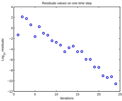
0 5 10 15 20 25 −12
−10 −8 −6 −4 −2 0 2 4
Residuals values on one time step
Iterations
Log
10
r
esiduals
Fig. 2. Sample residuals plotted for one time step.
5 Dam break experiments
One of the applications published in Martin and Gorelick (2005) is a dam break experiment. The experiment consists of a flume 21.2 m long and 1.4 m wide. The flume is closed at one end and open at the other end. It has a curved con-striction 5.0 m from the closed end that ends 4.7 m from the open end. A dam is located 8.5 m from the closed end, with an opening of width 0.6 m. The flume has a slope of 0.002 with water at a height of 0.15 m behind the dam (Martin and Gorelick, 2005).
Wave meters and pressure transducers were located at 8 locations, as seen in Fig. 3; however, the water depth mea-surements were only given in seven locations. The recorded water depths last for 62 s after the dam is broken. With the dam position chosen as the origin, the wave meters are lo-cated at placesx= −8.5,−4.5, and−0.0 m, and the pres-sure transducers are placed at x= +0.0, +2.5, +5.0, +7.5, and +10.0 m (Martin and Gorelick, 2005). The computational time step used in the experiment is1t=0.103 s and the grid dimensions are1x=0.05 m and 1y=0.125 m. With this grid cell size, the geometry is sliced into 30×171 grid cells. Finally, simulated water heights at the seven locations were compared with heights measured by the wave meters and pressure transducers.
5.1 VEnKF parameters
The state vector for the assimilation is defined as the vector of heights at the center of a grid point. The complete state vec-tor comprises the free surface elevationηand the horizontal velocitiesuin thexdirection andvin theydirection for the entire domain, i.e.,s= [η u v]T. The model has, therefore, altogether 16 000 spatial degrees of freedom. With the inter-polations described in Sect. 5.3, the ensembles are sampled in every time step of the assimilation. The observation error and the model error covariance matrices are both assumed
Fig. 3. Plan view flume layout for the dam break experiment of
Bellos et al. (1992). Wave meter locations are displayed with circles. Pressure transducer locations are displayed with triangles (Martin and Gorelick, 2005).
to be diagonal. The observation operatorHin Eq. (17) is a linear operator that maps the state vector to the observation space corresponding to all grid points covered by the inter-polated data, but restricted to the water height values only. 5.2 Experiment 1: VEnKF application to dam break
with synthetic data
The aim of this experiment is to examine both qualitative and quantitative characteristics of the VEnKF method to the dam break experiment. The data set has been generated by adding normally distributed noise with mean 0 and a variance of 5×
10−2from the solution of the model simulation. To make the experiment more realistic, data has been picked in 8 positions corresponding to wave meter locations defined in Martin and Gorelick (2005). More precisely, the time interval between the data in all locations was fixed, but chosen randomly for every location. This setup emulates the fact that wave meters do not necessarily collect information at the same time. 5.2.1 Results for experiment 1
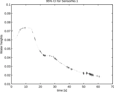
In Figs. 4 and 5, the matching between the data, VEnKF es-timates (50 ensembles) and the model simulation, here re-ferred to as the truth, is shown for all 8 wave meter locations. The target of the current study is not really data assimila-tion for the purpose of a subsequent forecast with VEnKF, as would be the case in an atmospheric dynamics context, but instead qualitatively better hind-casting of a catastrophic event such as a dam breaking down, with an ensemble-based approach. In our case, the length of each forecast is therefore just one computational time step at a time with interpolated observations. This close match between the model and ob-servations over one time step also results in very compact ensemble spreads, as can be seen in Fig. 6.
0 10 20 30 40 50 60 70 0.00
0.02 0.04 0.06 0.08 0.10 0.12 0.14
Time [s]
Height [m]
(a): SensorNo.1
VEnKF Truth Data
0 10 20 30 40 50 60 70 0.00
0.02 0.04 0.06 0.08 0.10 0.12 0.14
Time [s]
Height [m]
(b): SensorNo.2
VEnKF Truth Data
0 10 20 30 40 50 60 70 0.00
0.02 0.04 0.06 0.08 0.10 0.12 0.14
Time [s]
Height [m]
(c): SensorNo.3
VEnKF Truth Data
0 10 20 30 40 50 60 70 0.00
0.02 0.04 0.06 0.08 0.10 0.12 0.14
Time [s]
Height [m]
(d): SensorNo.4
VEnKF Truth Data
Fig. 4. Experiment 1: Comparison of VEnKF estimates, true water
depth and data of the dam break experiment for the first four sensors at the upstream end.
a period of 10 s from the begining of the experiment, as this period is the best one to display the error before water has started to run out from the flume.
5.3 Experiment 2: VEnKF for dam break experiment with real data
The published data set (see Martin and Gorelick, 2005) of measurements is used to assimilate water heights. The high sparsity of the set of measurements is challenging for data assimilation. Observations come at an average rate of 1.6 observations in one or more locations per time step and at a maximum of 5 locations per time step. They feature only measurements of water height. This means that the number of observations in relation to the dimension of state space is approximately 1/100 000, since the computational time step is 0.1 s. For this reason, the observations are interpo-lated in time by a spline scheme and in space by a Gaussian mask to make them dense enough for the VEnKF assimila-tion scheme. This means we interpolate the observaassimila-tions in time and extrapolate each of them in space by a Gaussian kernel. After this, the ratio of the number of observations to system dimension improves to 1/50.
5.3.1 Shore boundary definition for the VEnKF
As can be seen from the MAP estimate problem (17), the VEnKF does not account for additional prior knowledge be-yond the observations. This means that in the case of prob-lems on bounded domains, there is no way to include infor-mation about the boundaries in the Kalman filter analysis. If the prediction model automatically maintains the bound-aries in accordance with defined constraints, one can simply
0 10 20 30 40 50 60 70 0.00
0.02 0.04 0.06
Time [s]
Height [m]
(a): SensorNo.5
VEnKF Truth Data
0 10 20 30 40 50 60 70 0.00
0.02 0.04 0.06
Time [s]
Height [m]
(b): SensorNo.6
VEnKF Truth Data
0 10 20 30 40 50 60 70 0.00
0.02 0.04 0.06
Time [s]
Height [m]
(c): SensorNo.7
VEnKF Truth Data
0 10 20 30 40 50 60 70 0.00
0.02 0.04 0.06
Time [s]
Height [m]
(d): SensorNo.8
VEnKF Truth Data
Fig. 5. Experiment 1: Comparison of VEnKF estimates, true water
depth and data of the dam break experiment for the last four sensors.
0 10 20 30 40 50 60 70
0.01 0.02 0.03 0.04 0.05 0.06 0.07 0.08 0.09 0.1
95% CI for SensorNo.1
Water heights
time [s]
Fig. 6. 95 % confidence region is shown for the location of Sensor
No. 1.
reduce the data assimilation analysis to the inner part of the model domain. However, this approach is complicated when the boundaries change over time.
In our experiments, we use a strategy that allows us to account more flexibly for evolving boundaries, albeit with-out guaranteeing that the boundaries will be preserved ex-actly as required by the model constraints. Information about the boundaries is included in the model uncertainty descrip-tion, i.e., in the model error covarianceCεk(see Eq. 15). This
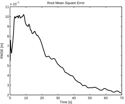
0 10 20 30 40 50 60 70 2
3 4 5 6 7 8 9 10
11x 10
−3
Time [s]
RMSE [m]
Root Mean Square Error
Fig. 7. The RMSE plot for the entire time of assimilation.
In the dam break case studied here, we have prior knowl-edge about the shoreline and there will be no water in places where there is a riverbank. Therefore, we define the model covarianceCεk such that the state elements that are confined
to the riverbank have variances much smaller than the vari-ances assigned to the rest of the state. This strategy shifts the responsibility of maintaining the boundaries to the data assimilation analysis.
6 Model applications with real data
6.1 Results without data assimilation
The results of direct model simulations with MOD-FreeSurf2D show that the simulated water depth matches well with the measured depth only for the three measurement locations above the dam (at the upstream end), as can be seen in Fig. 9a–c. The results are less accurate for other locations below the dam due to the emergence of super-critical flows in the downstream end. The downstream end is also character-ized by turbulent flow, and the model only tracks the height of water, but not the turbulent fine structure of the flow. In Fig. 9d as well as Fig. 10a and b in particular, we can see the discontinuity of the flow at the beginning of the dam opening. 6.2 Results with data assimilation
The model error and the observation error covariance matri-ces were set to Cεp
k
=(0.0011)2I and Cζk =(0.001) 2I,
re-spectively. We use the initial estimate of the statex0estequals the initial height of water and the initial covariance estimate
C0est=I.
Measurements are incorporated into the model, and the as-similation is done with an ensemble size of 75 members. The number of LBFGS iterations and stored vectors is set to 25. When the dam is removed, a strong flood wave is generated
0 0.5 1 1.5 2 2.5 3 3.5 4 4.5
0.009 0.0095 0.01 0.0105 0.011 0.0115 0.012
Time [s]
RMSE [m]
Forecast skill; about 4s ahead
Fig. 8. The forecast skill plot for about 4 s period of forecast
0 10 20 30 40 50 60 70 0.00
0.02 0.04 0.06 0.08 0.10 0.12 0.14 0.16 0.18 0.20
(a): SensorNo1
Time [s]
Height [m]
Simulation Data
0 10 20 30 40 50 60 70 0.00
0.02 0.04 0.06 0.08 0.10 0.12 0.14 0.16 0.18 0.20
(b): SensorNo2
Time [s]
Height [m]
Simulation Data
0 10 20 30 40 50 60 70 0.00
0.02 0.04 0.06 0.08 0.10 0.12 0.14 0.16
(c): SensorNo3
Time [s]
Height [m]
Simulation Data
0 10 20 30 40 50 60 70 0.00
0.02 0.04 0.06 0.08 0.10 0.12 0.14 0.16
(d): SensorNo4
Time [s]
Height [m]
Simulation Data
Fig. 9. Comparison of simulated water depth and measured depth of
the dam break experiment for the first four sensors at the upstream end.
and propagated downstream from the flume. The variation of water depth with time is compared with experimental data as given by the seven sensors; see Figs. 11 and 12.
From the results it can be seen that at the location imme-diately after the dam (location 4), the original simulation did not capture the behavior of the flow at the beginning of the simulation. However, VEnKF is able to approximate the wa-ter height and the structure of the flow. The same situation was observed in locations 5, 6 and 8, where the VEnKF re-sult captures well the most prominent features of the flow.
0 10 20 30 40 50 60 70 0.00 0.02 0.04 0.06 0.08 0.10 (a): SensorNo5 Time [s] Height [m] Simulation Data
0 10 20 30 40 50 60 70 0.00 0.02 0.04 0.06 0.08 0.10 (b): SensorNo6 Time [s] Height [m] Simulation Data
0 10 20 30 40 50 60 70 0.00 0.02 0.04 0.06 0.08 (c): SensorNo7 Time [s] Height [m] Simulation
0 10 20 30 40 50 60 70 0.00 0.02 0.04 0.06 0.08 (d): SensorNo8 Time [s] Height [m] Simulation Data
Fig. 10. Comparison of simulated water depth and measured depth
of the dam break experiment for the last four sensors at the down-stream end. Sensor No. 7 did not have measurements.
0 10 20 30 40 50 60 70 0.00 0.02 0.04 0.06 0.08 0.10 0.12 0.14 Time [s] Height [m] (a): SensorNo1 VEnKF Data
0 10 20 30 40 50 60 70 0.00 0.02 0.04 0.06 0.08 0.10 0.12 0.14 Time [s] Height [m] (b): SensorNo2 VEnKF Data
0 10 20 30 40 50 60 70 0.00 0.02 0.04 0.06 0.08 0.10 0.12 0.14 Time [s] Height [m] (c): SensorNo3 VEnKF Data
0 10 20 30 40 50 60 70 0.00 0.02 0.04 0.06 0.08 0.10 0.12 0.14 Time [s] Height [m] (d): SensorNo4 VEnKF Data
Fig. 11. Experiment 2: Comparison of VEnKF results and measured
depth of the dam break experiment for the first four sensors at the upstream end.
It is worth pointing out the time series of water heights at sensor 7 that did not provide any measurements because of a sensor malfunction. If we compare the simulated curve in Fig. 10c with direct simulation to that of Fig. 12c with data assimilation, we see that the latter contains similar fine scale oscillations due to small waves as the sensors with observa-tions, but that these oscillations are missing in Fig. 10c.
This demonstrates that the qualitative improvements to-wards a more realistic representation of the flume are not restricted to sites with observations, but are indeed spread throughout the computational domain. This can be seen in more detail in the accompanying videos that represent the
0 10 20 30 40 50 60 70 0.00 0.02 0.04 0.06 0.08 Time [s] Height [m] (a): SensorNo5 VEnKF Data
0 10 20 30 40 50 60 70 0.00 0.02 0.04 0.06 0.08 Time [s] Height [m] (b): SensorNo6 VEnKF Data
0 10 20 30 40 50 60 70 0.00 0.02 0.04 0.06 0.08 Time [s] Height [m] (c): SensorNo7 VEnKF
0 10 20 30 40 50 60 70 0.00 0.02 0.04 0.06 0.08 Time [s] Height [m] (d): SensorNo8 VEnKF Data
Fig. 12. Experiment 2: Comparison of VEnKF results and measured
depth of the dam break experiment for the last four sensors at the downstream end. Sensor No. 7 did not have measurements.
pure simulation and the flume obtained with data assimila-tion.
7 Discussion and conclusions
The use of data assimilation to complement forecasts made by mathematical models with observational data is a growing trend in scientific computing. This trend is likely to continue, since the computer capacity accessible to researchers is in-creasing rapidly, and many different kinds of automatic mea-surement devices are becoming available that provide large numbers of measurements from target systems.
In the foregoing sections, we have demonstrated some of the benefits that data assimilation can bring to hydrological modeling. The resulting analysis of a dam break flume be-haves in a more realistic manner than the corresponding com-puter simulation alone. It displays turbulent behavior such as the real flow, features prominent hydraulic jumps, and avoids several numerical artifacts.
Acknowledgements. Thanks to Lappeenranta University of Technology and the World Bank Project funding through the University of Dar es salaam and Dar es salaam University College of Education, without these funding this work would be impossible. Our thanks also go to the anonymous reviewers for their insightful review of our work.
Edited by: R. Buizza
Reviewed by: two anonymous referees
References
Aliparast, M.: Two-dimensional finite volume method for dam-break flow simulation, Int. J. Sediment Res., 24, 99–107, 2009. Auvinen, H., Bardsley, J., Haario, H., and Kauranne, T.: The
vari-ational Kalman filter and an efficient implementation using lim-ited memory BFGS, Int. J. Numer. Meth. Fl., 64, 314–335, 2009. Baghlani, A.: Simulation of dam-break problem by a robust flux-vector splitting approach in Cartesian grid, Scientia Iranica, 18, 1061–1068, 2011.
Barcena, J. F., Garcia, A., Garcia, J., Alvares, C., and Revilla, J. A.: Surface analysis of free surface and velocity to changes in river flow and tidal amplitude on a shallow mesotidal estuary: An ap-plication in Suances Estuary (Nothern Spain), J. Hydrol., 420– 421, 301–318, 2012.
Bardsley, J., Solonen, A., Parker, A., Haario, H., and Howard, M.: An Ensemble Kalman Filter Using the Conjugate Gradient Sampler, Int. J. Uncert. Quant., 3, 357–370, doi:10.1615/Int.J.UncertaintyQuantification.2012003889, 2013. Bates, P. and Anderson, M.: A two-dimensional finite-element
model for river flow inundation, P. Roy. Soc. Lond. A. Mat., 440, 481–491, doi:10.1098/rspa.1993.0029, 1993.
Bellos, C., Soulis, J., and Sakkas, J.: Computation of two-dimensional dam-break induced flows, Adv. Water Resour., 14, 31–41, 1991.
Casulli, V.: A Semi-implicit finite difference method for non hydro-static, free-surface flows, Int. J. Numer. Meth. Fl., 30, 425–440, 1999.
Casulli, V. and Cheng, R.: Semi-implicit finite difference methods for three-dimensional shallow water flow, Int. J. Numer. Meth. Fl., 15, 629–648, doi:10.1002/fld.1650150602, 1992.
Courtier, P. and Talagrand, O.: Variational assimilation of meteo-rological observations with the adjoint vorticity equation, Part 2: Numerical results, Q. J. Roy. Meteor. Soc., 113, 1329–1368, 1987.
Daley, R.: Atmospheric Data Analysis, Cambridge University Press, 1st Edn., 1991.
Drikakis, D. and Tsangaris, S.: On the solution of the compress-ible Navier-Stokes equations using improved flux vector splitting methods, Appl. Math. Model., 17, 282–297, 1993.
Erpicum, S., Dewals, B., Archambeau, P., and Pirotton, M.: Dam break flow computation based on an efficient flux vector splitting, J. Comput. Appl. Math., 234, 2143–2151, 2010.
Evensen, G.: Sequential data assimilation with a nonlinear quasi-geostrophic model using Monte-Carlo methods to forecast error statistics, J. Geophys. Res., 99, 10143–10162, 1994.
Goldstein, S.: Modern developments in fluid mechanics, Oxford Univ. Press, 1938.
Heniche, M., Secretan, Y., Boudreau., P., and Leclerc, M.: Two-dimensional finite volume model for dam-break simulation, Adv. Water Resour., 23, 359–372, 2000.
Kalman, R.: A new approach to linear filtering and prediction prob-lems. Transaction of the ASME, J. Basic Eng.-T. ASME, 82, 35– 45, 1960.
Le Dimet, F.-X. and Talagrand, O.: Variational algorithms for anal-ysis and assimilation of meteorological observations: theoretical aspects, Tellus, 38A, 97–110, 1986.
Lewis, J. M. and Derber, J. C.: The use of adjoint equations to solve a variational adjustment problem with advective constraints, Tel-lus, 37A, 309–322, 1985.
Lorenc, A.: Analysis methods for numerical weather prediction, Q. J. Roy. Meteor. Soc., 112, 1177–1194, 1986.
Martin, N. and Gorelick, S. M.: MODFreeSurf2D: A MATLAB sur-face fluid flow model for rivers and streams, Comput. Geosci., 31, 926–946, 2005.
Nocedal, J. and Wright, S.: Numerical Optimization, chap. Limited-Memory BFGS, Springer-Verlag, New York, 224–227, 1999. Simon, D.: Optimal state estimation, Kalman,H∞, and nonlinear
approaches, Wiley-Interscience, Hoboken, 2006.
Solonen, A., Haario, H., Hakkarainen, J., Auvinen, H., Amour, I., and Kauranne, T.: Variational ensemble Kalman filtering using limited memory BFGS, Electron T. Numer. Ana., 39, 271–285, 2012.
Toro, E. and Vazquez-Cendon, M.: Flux splitting schemes for the Euler equations, Comput. Fluids, 70, 1–12, 2012.
Ying, X., Jorgeson, J., and Wang, S.: Modeling Dam-Break flows using Finite Volume method on unstructured grid, Eng. Appl. Comput. Fluid Mech., 3, 184–194, 2009.
Yoon, T. and Kang, S.: Finite volume model for two-dimensional shallow water flows on unstructured grids, J. Hydraul. Eng.-ASCE, 130, 678–688, 2004.
Zhang, M. and Wu, W.: A two dimensional hydrodynamic and sediment transport model for dam break based on finite vol-ume method with quadtree grid, Appl. Ocean Res., 33, 297–308, 2011.