A. Ganopolski1, R. Calov1, and M. Claussen2,3
1Potsdam Institute for Climate Impact Research, Potsdam, Germany 2Max Planck Institute for Meteorology, Hamburg, Germany 3KlimaCampus University Hamburg, Hamburg, Germany
Received: 9 September 2009 – Published in Clim. Past Discuss.: 12 October 2009 Revised: 18 March 2010 – Accepted: 31 March 2010 – Published: 13 April 2010
Abstract. A new version of the Earth system model of intermediate complexity, CLIMBER-2, which includes the three-dimensional polythermal ice-sheet model SICOPOLIS, is used to simulate the last glacial cycle forced by varia-tions of the Earth’s orbital parameters and atmospheric con-centration of major greenhouse gases. The climate and ice-sheet components of the model are coupled bi-directionally through a physically-based surface energy and mass balance interface. The model accounts for the time-dependent effect of aeolian dust on planetary and snow albedo. The model successfully simulates the temporal and spatial dynamics of the major Northern Hemisphere (NH) ice sheets, including rapid glacial inception and strong asymmetry between the ice-sheet growth phase and glacial termination. Spatial ex-tent and elevation of the ice sheets during the last glacial maximum agree reasonably well with palaeoclimate recon-structions. A suite of sensitivity experiments demonstrates that simulated ice-sheet evolution during the last glacial cy-cle is very sensitive to some parameters of the surface energy and mass-balance interface and dust module. The possibility of a considerable acceleration of the climate ice-sheet model is discussed.
1 Introduction
Simulation and understanding of glacial cycles, which dom-inated climate variability over the past several million years, still remain a major scientific challenge. Although a large body of palaeoclimate evidences supports the hypothesis of the Earth’s orbital variations as pacemaker for glacial cycles, a number of scientific questions remain unsolved. Among
Correspondence to: A. Ganopolski
POTSDAM
Statistical-Dynamical Atmosphere Model
Land Surface Model
Ocean Model
SEMI Surface Energy and
Mass Balance Interface
DUSTER Dust Model
SICOPOLIS Ice Sheets Model
T, P, SWR, LWR, WND, CLD
iMBL iTSUR
iCAL
iVOL, iMLT iMASK, iSLD
RDST
iELV, SL, iFRC , iMLT
DDST
Fig. 1. Flow diagram of the model version used in this study. Thick
arrows represent new flows of information compared to the “stan-dard” version of CLIMBER-2 described in Petoukhov et al. (2000). Abbreviations are explained in the Table 1.
In recent years, a new class of models, the so-called Earth system model of intermediate complexity (EMICs; Claussen et al., 2002) became available for the study of glacial cy-cles. These models are far less computationally demand-ing than coupled GCMs but incorporate substantially more physical processes than simple models. In particular, several EMICs simulate the most recent glacial inception (around 120–115 kyr BP) with reasonable agreement with palaeo-data, at least, in respect of the total ice volume (Wang and Mysak, 2002; Calov et al. 2005). A stability analysis of the climate-cryosphere system performed by Calov and Ganopolski (2005) has shown that the glacial inception rep-resents a bifurcation transition in the climate-cryosphere sys-tem and that the climate syssys-tem possesses multiple equilibria within the range of Milankovitch forcing, thus supporting the nonlinear paradigm proposed by Paillard (1998, 2001). Re-cently, the entire last glacial cycle was simulated with the same climate model used in this study, but coupled to an-other ice sheet model and using a different coupling tech-nique (Bonelli et al., 2009).
The purpose of our paper is to present the results of our simulations of the last glacial cycle with the CLIMBER-2 model, where the climate and ice-sheet components are coupled bi-directionally using a physically-based surface en-ergy and mass balance interface. This work represents a continuation of our previous work (Calov et al., 2005), but with an improved version of the model. It is important to note that in this work, similar to previous modelling studies, we prescribed time-dependent radiative forcing of the ma-jor greenhouse gases, in addition to orbital forcing. Such a modelling experiment represents an important test for the climate-cryosphere model, but cannot be considered as a de-cisive test for the Milankovitch theory, since, in the real world, changes in the greenhouse gas concentration are not an external forcing, but rather an important internal feedback in the Earth system.
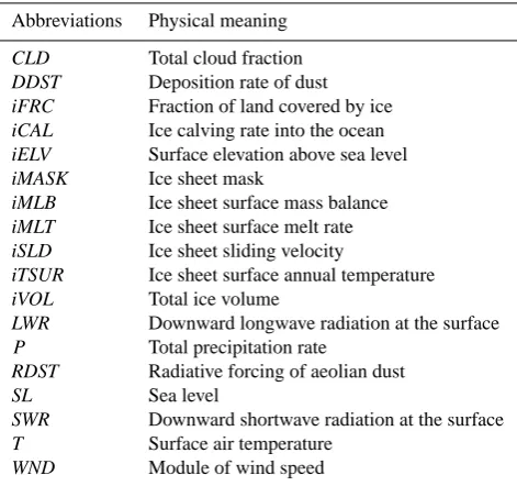
Table 1. Abbreviations of information fluxes shown in Fig. 1.
Abbreviations Physical meaning
CLD Total cloud fraction
DDST Deposition rate of dust
iFRC Fraction of land covered by ice
iCAL Ice calving rate into the ocean
iELV Surface elevation above sea level
iMASK Ice sheet mask
iMLB Ice sheet surface mass balance
iMLT Ice sheet surface melt rate
iSLD Ice sheet sliding velocity
iTSUR Ice sheet surface annual temperature
iVOL Total ice volume
LWR Downward longwave radiation at the surface
P Total precipitation rate
RDST Radiative forcing of aeolian dust
SL Sea level
SWR Downward shortwave radiation at the surface
T Surface air temperature
WND Module of wind speed
2 Model description
The model used for this study is the newest version of CLIMBER-2. It is similar to that described by Calov et al. (2005) (hereafter C05). Since the model and its perfor-mance has been described in a number of previous publica-tions, here we give only a short, general description and will discuss in more detail only the essential improvements com-pared to the version used in C05.
similar to C05, we applied the dust deposition rate based on results of simulations for the present-day and LGM (Last Glacial Maximum) conditions by Mahowald et al. (1999). In addition, we implement a parameterisation for the dust de-position originating from glacial erosion in the model. This is, according to Mahowald et al. (2006a), an important ad-ditional source of dust in the vicinity of the ice sheets. We also explicitly included the direct radiative forcing of atmo-spheric dust in the same way as Schneider et al. (2006). As in C05, the cryosphere component affects climate via changes in the fraction of grid cell covered by ice, which affect sur-face albedo, elevation and land fraction for each grid cell of the coarse resolution climate component of the CLIMBER-2 model. Note that although the fractions of grid cells covered by the ice sheets change only in the NH; changes in eleva-tion and land fraceleva-tions caused by sea-level variaeleva-tions were applied to all model grid cells. In the present work, we ad-ditionally accounted for the freshwater flux into the ocean originating from the ice sheets with explicit coupling of the ice-sheet module to the ocean module. In the following sec-tions, we will describe the most important model improve-ments compared to the model version used in C05.
2.1 Freshwater flux from the ice sheets
Changes in freshwater flux into the ocean caused by growth and decay of the ice sheets primarily affect climate via changes of the Atlantic meridional overturning circulation (AMOC), which is associated with meridional oceanic heat transport and sea ice cover. In particular, a reduction of the freshwater into the ocean contributes to a strengthening of the AMOC during rapid growth of the ice sheets, while dur-ing episodes of massive ice surges into the ocean (Heinrich events) and glacial terminations, an increased freshwater flux into the ocean leads to a weakening, or even a complete ces-sation of the AMOC, which affects climate in the North At-lantic realm considerably. Surface melting of ice sheets and iceberg calving into the ocean are simulated by the ice-sheet module. Surface ice-sheet melting is now added to the river runoff simulated by the climate component of the model, and calving is treated as surface freshwater flux into the near-est oceanic grid cell. During glacial time, the river routing differed from the present configuration and was evolving in time. Hence, in principle, the river routing scheme should be updated regularly taking into account changes in the ice-sheet distribution and land elevation. However, for simplicity
sideration and all meltwater from the ice sheets is released into the ocean immediately. Note, that both meltwater and iceberg calving are treated as surface freshwater flux and, hence, the potential effect of penetration of meltwater into the deep ocean with sediment-laden flow (e.g. Roche et al., 2007) is not accounted for.
2.2 Radiative forcing of atmospheric dust
Palaeoclimate data indicate that the amount of dust in the atmosphere during glacial times was considerably higher than during interglacials. Modelling studies suggest that en-hanced atmospheric dust content during glacial time repre-sented an important additional radiative forcing component (e.g. Claquin et al., 2003). This forcing was extremely in-homogeneous spatially and varied seasonally. Recent esti-mates with GCMs indicate that the globally averaged radia-tive forcing of atmospheric dust during the LGM has an or-der of magnitude of−1 W/m2, and according to simulations by Mahowald et al. (2006b) and Schneider et al. (2006), it caused an additional global cooling effect of about 0.5 to 1◦C with a stronger cooling in the NH. Note that this is only ra-diative (shortwave and longwave) forcing of the dust in the atmosphere. The impact of dust on snow albedo was treated separately (see below). Since the simulations of atmospheric dust radiative forcing are only available so far for the LGM time slice, a parameterisation is needed for the evolution of radiative forcing of the atmospheric dust in the transient ex-periments. We applied a similar procedure to prescribe the temporal development of radiative dust forcing, as that which was used in C05 for the dust deposition rate. Namely, we assume that the additional (compared to the present one) ra-diative forcing of dustRd is proportional to the global ice volume as
Rd=Rd
LGMV /VLGM, (1)
the atmosphere but also on surface albedo, which changed considerably during the glacial cycle. These problems can only be avoided by the incorporation of the dust cycle di-rectly into the CLIMBER-2 model, work which is now in progress.
2.3 Dust deposition rate
It has already been shown by Warren and Wiscombe (1980) that even a tiny amount of dust (relative concentrations of about 100 parts per million of weight, ppmw) mixed with snow decreases the albedo of fresh snow by 0.1. For old snow, this reduction can even reach 0.3. In their initial growth phase, the major NH ice sheets occurred in areas with rather small dust deposition rates. But during the latter stages of the glacial cycle, the ice sheets spread into areas where dust deposition rates, especially under glacial conditions, be-came sufficient to appreciably affect the albedo of snow. As was shown in C05 and confirmed using a more sophisticated model by Krinner et al. (2006), accounting for the effect of dust on snow albedo prevents the growth of the ice sheets in areas with high dust deposition rates, such as Eastern Siberia. Probably even more importantly, the impact of dust on snow albedo is related to the dust produced due to glacial erosion. According to empirical data (Mahowald et al., 2006a), the dust deposition rate associated with this mechanism was as high as 10 to 100 g/m2/yr just south of the North American and northern European ice sheets. If a typical annual precip-itation of about 500 mm/yr is assumed in these areas, such dust deposition rates would result in average concentration of dust in snow of 20 to 200 ppmw, assuming that dust is uni-formly mixed with snow over the whole year. In reality, most of the dust associated with glacial erosion is deposited during summer; hence, the concentration of dust in the upper snow layer during snowmelt is expected to be much higher than it would be in case of uniform mixing over the year. More-over, when snow melts, only a fraction of dust is removed by meltwater and therefore the concentration of dust in snow in-creases with time. Although the accurate modelling of all of these processes is problematic, related uncertainties are not crucial, because a saturation effect occurs for dust concen-tration in snow of more than 1000 ppmw and the albedo of snow reaches a value comparable to that for dirty ice.
In C05, we implemented a simple technique similar to Eq. (1), which produces a spatial distribution of dust depo-sition rates at any location using results of present-day and LGM simulations from Mahowald et al. (1999), proportion-ally weighted to the simulated global ice volume. Such an approach, however, is not justified for the glaciogenic dust, because the sources of glaciogenic dust (and therefore its de-position) are strongly related to the extent of the ice sheets and their internal dynamics. Therefore, it is not justified to apply glaciogenic dust simulated for the LGM ice sheets to other periods with very different configurations of the ice sheets. To resolve this problem, we introduced, in our model,
a rather simple parameterisation of dust deposition produced from the glaciogenic sources. This parameterisation is based on the assumption that the emission of glaciogenic dust is proportional to the delivery of glacial sediments to the edge of an ice sheet (see Appendix A for details). Most of the glaciogenic dust originates from the southern flanks of the ice sheets and this source is significant only for mature ice sheets, which reach well into areas covered by thick terres-trial sediments. Parameters of the glaciogenic dust module were tuned to reproduce the reconstructed rate of dust de-position during the LGM. Simulated glaciogenic dust was added to the dust deposition rate taken from Mahowald et al. (1999). Note that Mahowald et al. (1999) did not account for glaciogenic dust sources.
2.4 Sliding parameterisation
As shown by modelling studies by Calov et al. (2002) and Calov and Ganopolski (2005), fast sliding processes over ar-eas covered by deformable sediments play an important role in ice-sheet dynamics, both on millennial and longer time scales. In the current work, we use three types of surfaces underlying the ice sheets: rocks, deformable terrestrial sedi-ments and marine sedisedi-ments. The first two types correspond to present-day land and were distinguished by prescribing a minimum sediment layer thickness in the data source by Laske and Masters (1997), while all areas which lay below present-day sea level were considered to be covered by ma-rine sediments. Basal sliding appears only if the base of an ice sheet is at the pressure melting point, in which case, the sediment type of underlying surface becomes important. Two different sliding laws were applied for rock (Calov and Hutter, 1996) and sediment (C05), while the difference be-tween terrestrial and marine sediment was represented by the value of the sliding parameter, which is an order of magni-tude higher for marine sediment.
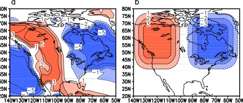
2.5 Temperature correction for North America
Fig. 2. (a) Deviation of observed summer surface air temperature from the zonal average over the CLIMBER-2 sector corresponding to
North America. (b) Temperature correction added to the interpolated CLIMBER-2 temperature in the SEMI module.
demonstrated that the lack of this zonal gradient causes a problem for the realistic simulations of the North American ice sheets (see also the discussion in Sect. 6). Thereby, we implemented a sub-grid correction for the atmospheric tem-perature in the North American sector, which has the shape of a dipole and closely resembles the deviations of the observed summer air temperature (corrected for elevation effect) from its zonal mean over North America (Fig. 2). The maximum of this applied temperature correction is 3◦C. Although this temperature structure is more representative for the summer season, we kept the temperature correction constant in time, since it is the summer temperature that is most important for the mass balance of an ice sheet. The temperature correction was added to the surface air temperature interpolated from the coarse climate module grid. This temperature correction directly affects the surface sensible heat flux and, in addi-tion, the downward longwave radiation by assuming a linear relationship between temperature and downward longwave radiation.
3 Experimental setup
Similar to C05, the model was forced by variations in orbital parameters computed following Berger (1978) and green-house gas (GHG) concentrations derived from the Vostok ice core. Unlike C05, we now account for two other im-portant GHGs: CH4and N2O. Since the radiative scheme of the CLIMBER-2 model does not include CH4and N2O, the radiative effect of these gases was incorporated via the so-called equivalent CO2concentration, which is determined as the CO2concentration which has the same radiative forcing as the combined radiative forcing of all major greenhouse gases (see Appendix B for details). All model runs started from the equilibrium state corresponding to the orbital con-figuration and the concentration of GHGs at 126 kyr BP. The model then was run fully interactively and synchronously for
126 000 years until present-day, thus covering the whole last glacial cycle.
We will start the discussion of modelling results with a so-called Baseline Experiment (BE). This experiment repre-sents a “suboptimal” subjective tuning of the model parame-ters to achieve the best agreement between modelling results and palaeoclimate data. Obviously, even with a model of in-termediate complexity it is not possible to test all possible combinations of important model parameters which can be considered as free (tunable) parameters. In fact, the BE was selected from hundred model simulations of the last glacial cycle with different combinations of key model parameters. Note, that we consider “tunable” parameters only for the ice-sheet model and the SEMI interface, while the utilized climate component of CLIMBER-2 is the same in previous studies, such as those used by C05. In the next section, we will discuss the results of a set of sensitivity experiments, which show that our modelling results are rather sensitive to the choice of the model parameters. Therefore, the simula-tion of a realistic glacial cycle would represent a too ambi-tious task if the model was too computationally expensive to perform a large set of experiments. The selection of the best fit to the palaeodata is based on several criteria, among which are an accurate simulation of the total ice-volume variations over the whole glacial cycle, and an agreement between sim-ulated and reconstructed ice sheets during LGM. It is impor-tant to note that some systematic biases exist in all model simulations; we were not able to eliminate them with any combination of the model parameters.
4 Baseline experiment 4.1 Ice-sheet evolution
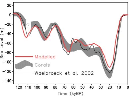
Fig. 3. Simulated and reconstructed sea-level evolution during the
last glacial cycle, relative to present-day values. The red line shows the sum of the simulated Northern Hemisphere (NH) ice volume and the contribution of the Antarctic Ice Sheet (following Huy-brechts, 2002), expressed in units of sea level change. The grey area represents an interpretation of recent coral data compilations (Lam-beck et al., 2002; Thompson and Goldstein, 2006; supplementary data therein). The width of the interval corresponds to two standard deviations. A very small number of well-dated corals for MIS 5d preclude a reliable estimate of the sea level from corals for this pe-riod. The solid black line shows the reconstruction by Waelbroeck et al. (2002) based on deep oceanδ18Ocand temperature records.
several palaeoclimate reconstructions. When we compared the model results with sea-level change reconstructions, the problem was that our model does not account for the South-ern Hemisphere ice sheets, which, in accordance with dif-ferent estimates, contributed an additional of ca. 20 m to the LGM sea-level drop. This contribution, estimated by Huy-brechts (2002), was added to the modelled NH ice volume and plotted in the figure together with an estimate of the range of sea-level variations based on recent coral data com-pilations (Lambeck et al., 2002; Thompson and Goldstein, 2006; supplementary data therein) and an independent es-timate of sea-level change based onδ18Oc and deep ocean
temperature (Waelbroeck et al., 2002). As seen in the figure, the model simulates all major aspect of the ice-volume varia-tions during the whole glacial cycle in reasonable agreement with palaeoclimate estimates. As compared to most previous simulations of the last glacial cycle based on different mod-elling approaches (e.g. Tarasov and Peltier, 1997; Marshall and Clark, 2002; Zweck and Huybrechts, 2004; Abe-Ouchi, 2007; Charbit et al. 2007; Bonelli et al., 2009), our model simulate much more pronounced (and, in generally, more re-alistic) variations in the ice volume on the precessional time scale (ca. 20 kyr). This is likely to be explained by fact that the previous modelling studies employed the positive degree day approach, which only indirectly accounts for insolation changes. In our model, the mass balance of the ice sheets is computed using a surface energy balance approach, which is more sensitive to variations in insolation.
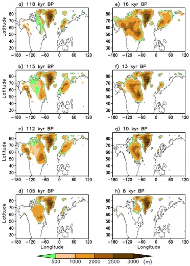
Similarly to C05, initial buildup of the ice sheets dur-ing the last glacial inception starts soon after 120 kyr BP in Scandinavia, Arctic Archipelago and Labrador (Fig. 4a). Al-ready around 112 kyr BP (Fig. 4c), the ice volume reaches 50 meters in sea-level equivalent (msl). During warm stages MIS 5c (Fig. 4d) and 5a most of the European ice sheets dis-appeared, whilst a relatively large ice sheet survived in the eastern part of North America. The magnitude of ice volume variations during MIS 5 as well as the steep rise of the ice sheets during MIS 4 are correctly simulated by the model. During most of MIS 3 the model simulate a relatively sta-ble ice volume and the rise of the ice volume resume around 30 kyr BP, in agreement with palaeoclimate data. The max-imum NH ice volume of ca. 90 msl was reached at around 20 kyr BP, i.e. one to several thousand years later than in-dicated by palaeoclimate reconstructions. At the LGM, the North American ice sheets contribute about 70 m to global sea-level drop, while the northern European ice sheet con-tributes slightly below 20 m. The glaciation in the east-ern Siberia, which developed shortly before the LGM, con-tributes only several meters. The spatial extent of simulated North American ice sheets (Fig. 5a) is close to the palaeo-climate reconstructions. In particular, east-western gradient in the position of the southern margin of North American ice complex is captured well. Compared to ICE-5G reconstruc-tion (Fig. 5b) by Peltier (2004) the elongated ice dome in the middle of the simulated Laurentide ice sheet is too thin, although our model captures the major topology of this struc-ture. Compared to the palaeoclimate reconstructions, simu-lated glaciation of Alaska is excessive. The extent and ice thickness of the Fennoscandian ice sheet, the south-western part of the European ice complex, are in good agreement with the ICE-5G reconstruction, while the north-eastern part of this ice complex does not reach far enough to the east, i.e. there is only a limited ice cover over Kara sea in the simulations.
Deglaciation of the NH began soon after 20 kyr BP and accelerates significantly after 16 kyr BP. Between 16 kyr BP and 14 kyr BP the averaged rate of ice-sheet melting reaches 15 msl per thousand years, which is comparable, though still smaller, than observed rate of sea-level rise during the MWP-1A event. During termination, the large portion of the Euro-pean ice sheets in the response to rising summer insolation and GHG concentration disappear before 13 kyr BP (Fig. 4f) and the most of the remaining European ice sheet melted prior to 10 kyr BP (Fig. 4g), which is ca. 1 kyr too early compared to palaeoclimate reconstructions. The initial re-sponse of the Laurentide ice sheet is slower and only around 15 kyr BP does its retreat accelerate significantly. At around 13 ky BP (Fig. 4f), the Laurentide and Cordilleran ice sheets separated and the remains of Laurentide ice sheet on Baffin Island (Fig. 4h) completely disappear soon after 8 kyr BP.
Fig. 4. Spatial extent and elevation of simulated ice sheets at different time slices during MIS 5: (a) 118 kyr BP, (b) 115 kyr BP, (c) 112 kyr BP, (d) 105 kyr BP, and during last glacial termination: (e) 16 kyr BP, (f) 13 kyr BP, (g) 10 kyr BP, (h) 8 kyr BP.
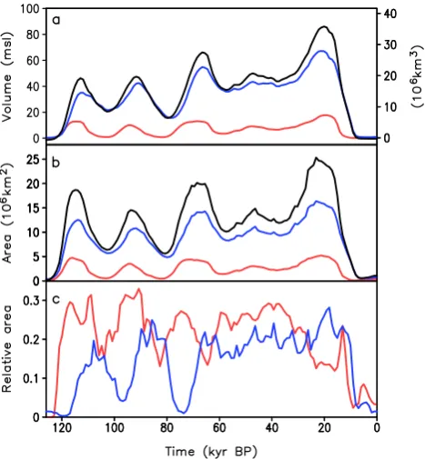
experiences stronger variability with the precessional period and it almost completely vanishes during MIS 5c and MIS 5a (Fig. 6a). The North American ice sheets are also affected by precessional variations but it survived periods of high sum-mer insolation and has a general tendency of growth through the whole glacial cycle. The area of the NH ice sheets closely follows NH ice volume except for the periods of rapid glacial
Fig. 5. Spatial extent and elevation of (a) simulated and (b) reconstructed (Peltier, 2004) ice sheets at the LGM.
Fig. 6. Simulated NH time series. (a) Ice volume, (b) ice area and (c) fraction of the ice sheets temperate basal area. The black line
shows the time series of the entire NH, the blue line of the North American and the red line of the European ice sheets.
melting point (temperate basal area). The relative fraction of the temperate basal area of the North American ice sheets, in spite of large fluctuations, has a tendency to increase towards the end of the glacial cycle, which is qualitatively similar to results by Marshall and Clark (2002). At the onset of glacial termination, almost one third of the ice-sheet area is tem-perate at the base; this contributes to rapid deglaciation due to fast sliding of the ice at the southern margins of the ice sheets.
Fig. 7. Simulated components of the mass balance of the NH ice sheets. (a) Total accumulation (solid blue) and ice-sheet area (dashed black). (b) Total surface melting (blue) and maximum sum-mer insolation at 65◦N (red dashed line). (c) Total ice calving. Units are Sverdrups of water (1 Sv=106m3/s).
The peak in the ablation rate of about 0.3 Sv during deglacia-tion at around 15 kyr BP is associated with the rapid resump-tion of the Atlantic thermohaline circularesump-tion (see Fig. 8), which causes pronounced warming over the North Atlantic realm.
Simulated ice sheet calving is rather noisy, which is partly attributed to the numerics of the ice sheet model. For this reason, the total calving rate shown in Fig. 7 is smoothed by a 10 year running-mean window. Still, it reveals strong tem-poral variability; the most pronounced of which is related to the large-scale instability of the Laurentide ice sheet via a mechanism described by Calov et al. (2002) and which re-sembles in many respects real Heinrich events. During these simulated ice surges, the calving rate exceeds 0.1 Sv. Al-though ablation remains the major negative contribution to the mass balance of the ice sheets over the whole glacial cy-cle, ice calving plays an important role in the millennial scale variability of AMOC.
4.2 Climate evolution
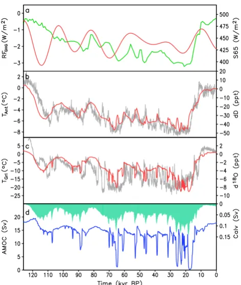
As shown with the CLIMBER-2 model in previous studies (Ganopolski, 2003; Schneider et al., 2006), approximately half of the global cooling (compared to present) during the last glacial maximum is explained by the presence of the large ice sheets in the NH and the rest by a lowering of the concentrations of the major GHGs (primarily CO2), an in-crease in atmospheric dust content and a shrinking of vege-tation cover. Since all of these factors are closely related and have a similar temporal dynamics, it is not surprising that the temporal evolution of the globally averaged annual sur-face air temperature during the glacial cycle follows the same pattern as the ice volume and CO2. On regional scale, how-ever, the temperature variations are more complicated and diverse. The northern North Atlantic temperature, which we consider as a proxy for Greenland temperature, apart from strong variations on orbital time scales, experienced numer-ous abrupt changes with a magnitude of up to 10◦C during a large portion of the glacial cycle (Fig. 8). In many re-spects, these tooth-shaped fluctuations resemble Dansgaard-Oeschger events recorded in numerous locations over the NH. Such fluctuations are attributed to rapid reorganisations of the Atlantic Meridional Overturning Circulation (AMOC). The largest perturbation of the AMOC, when circulation al-most stalled, coincides with the quasi-regular ice surges from the Laurentide ice sheet discussed by Calov et al. (2002).
Fig. 8. Climate forcing and climate evolution. (a) Prescribed
radia-tive forcing of GHGs (green) and orbital forcing (red) represented by changes in maximum summer insolation at 65◦N. (b) Simulated annual anomalies of East Antarctic temperature (red) and anomaly of the deuterium concentration from the EPICA ice core (grey).
(c) Simulated annual anomalies of the North Atlantic (60◦–70◦N) temperature (red) and measured anomaly of theδ18O concentration from the NGRIP ice core (grey). (d) Simulated rate of Atlantic out-flow at 30◦S (blue) and total ice calving (green). Note the reverse direction of y-axis for the ice calving. The anomalies in (b) and (c) are relative to present-day. Although the empirical data are ar-bitrarily scaled to achieve the best fit with the modelled data, the relationships between temperature variations and isotope variations are close to those used for palaeoclimate reconstructions.
Due to the random nature of millennial-scale variability, one cannot expect one-to-one correspondence between simulated and reconstructed temperatures. For example, the model equivalent of Bølling-Allerød occurs thousand years early than in reality. However, the overall qualitative agreement between model and data is quite instructive.
Fig. 9. Annual background dust deposition rates for (a) modern conditions and (b) LGM conditions based on Mahowald et al. (1999). (c)
Simulated glaciogenic dust deposition rate at the LGM, and (d) total dust deposition rate at the LGM equal to sum of the fields shown in (b) and (c).
As discussed above and illustrated by simulations de-scribed below, dust deposition plays an important role in the simulation of the glacial cycle with our model. As shown in Fig. 9a, d, dust deposition over the NH extra-tropics was significantly higher at the LGM as compared to the inter-glacial state. While outside of the ice sheets, the dust de-position is prescribed by the weighted mean of modern and LGM dust deposition rates simulated in Mahowald (1999) (Fig. 9b), the glaciogenic sources of dust play the dominant role in the vicinity of the ice sheets (Fig. 9c). At the LGM, the simulated values of dust deposition rates just south of both major NH ice complexes exceed 50 g/(m2yr), which is compatible with empirical data presented in Mahowald et al. (2006a). As shown in Fig. 10, the dust deposition rate south of the European and North American ice sheets ex-perienced variations with precessional period. However, in Europe the peaks in dust deposition are of similar magni-tude. The dust deposition rate south of Northern American ice sheet is much higher during LGM, which is explained by the fact that only prior to glacial termination a large portion of the Laurentide ice sheet spreads into the area covered by terrestrial sediments. Simulated dust deposition rate reduced snow albedo significantly and facilitated the retreat of the ice sheets during deglaciation.
5 Sensitivity experiments
The ice sheet model and the ice sheet-climate interface con-tain a number of parameters which are not derived from first principles. They can be considered as “tunable” parameters. As stated above, the BE was subjectively selected from a large suite of experiments as the best fit to empirical data. Be-low we will discuss results of a number of additional experi-ments illustrating the sensitivity of simulated glacial cycle to several model parameters. These results show that the model is rather sensitive to a number of poorly constrained param-eters and parameterisations, demonstrating the challenges to realistic simulations of glacial cycles with a comprehensive Earth system model.
Fig. 10. Simulated temporal evolution of annual dust deposition
rates in the grid cell south of the Laurentide Ice sheet (blue) and south of Fennoscandian ice sheet (red). The locations of the grid cells are shown in Fig. 9d by rectangles of corresponding colours.
sheet by ice advection. Considering the dust deposition data by Mahowald et al. (1999, 2006a), it becomes obvious that the enhancement factor could be much higher for the NH ice sheets, in particular, during glacial times. The other free pa-rameter determines the bottom sliding over the areas where the base of the ice sheet is temperate.
Experiments where the enhancement factor ranges be-tween 3 and 12 show a rather weak sensitivity of simulated glacial cycles to this parameter (Fig. 11a). This is explained by the relatively minor contribution of the deformation ve-locities, among other factors controlled by the enhancement factor, to the ice-sheet movement, as compared to basal slid-ing. Another reason for the low sensitivity of the ice dynam-ics to the enhancement factor lies in the ice-flow temperature coupling: if modelled ice velocities increase due to a higher enhancement factor, the ice sheet becomes cooler overall, be-cause colder and less deformable ice is advected downward, which, in turn, counteracts the velocity increase due to the enhancement factor. Doubling of the bedrock relaxation time scale (not shown) has a similarly small effect on global ice volume. In contrast, the sensitivity to the parameterisation of sliding processes is rather strong. The experiment where all continental grid points are treated as rocks differs consider-ably to the experiment where all continental grid points are treated as terrestrial sediments (Fig. 11a). In the first case, even when basal temperature is at the pressure melting point, the bottom sliding is rather small and the ice sheet reached at the LGM a much larger thickness than in the BE. In addition, due to much smaller rate of dust deposition simulated in this experiment, complete deglaciation of the NH is delayed by ca. 5 kyr compare to BE. In the experiment where all conti-nents are covered by terrestrial sediments, the ice sheets are much more mobile and considerably thinner than in the BE. As a result, during periods of high summer insolation, the ice sheets vanished completely and regrow only during periods when precessional variations of summer insolation are rein-forced by low obliquity. Hence, the simulated glacial cycle is rather sensitive to the parameterisation of bottom sliding, a process which is not yet properly understood.
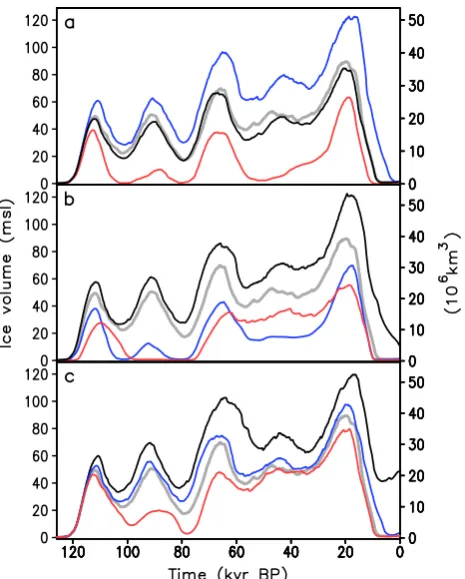
Fig. 11. Simulated NH ice volume in a suite of sensitivity
exper-iments. Grey lines in all figures show the Baseline Experiment.
(a) Sensitivity to ice-sheet-model parameterisations. The black line
corresponds to the enhancement-factor value 12 (the value used in BE is 3), the blue line corresponds to the experiment without terres-trial sediments, the red line to the experiment where all land is cov-ered by terrestrial sediments. (b) Sensitivity to parameterisations of the surface energy and mass balance interface. The black line cor-responds to the experiment without parameterisation of elevation-desert effect, the blue line corresponds to the experiment without effect of elevation slope on precipitation, and the red line represents the experiment without the North American temperature dipole cor-rection. (c) Sensitivity to the effect of the glaciogenic dust deposi-tion. The black line represents the experiment without the effect of dust deposition on snow albedo, the blue line with a halved and the red line with doubled amounts of the glaciogenic dust deposition.
5.2 Sensitivity to the parameters of the surface energy and mass balance interface
(40% higher at the LGM). As a result, the NH ice sheets did not disappear completely at the end of the simulation. To the contrary, switching off the parameterisation of slope effect on precipitation (Eq. 6 in C05), which leads to a reduction of the precipitation over the marginal parts of the ice sheets, considerably slows down the ice sheet growth. As a result, NH ice sheets vanished completely between 100 kyr BP and 80 kyr BP and reaches only a half of its LGM volume com-pared to BE.
Another attempt to correct unresolved regional climate pattern is the “American temperature dipole” described above. Although, the magnitude of this temperature correc-tion is only 3◦C, which is comparable to the typical temper-ature biases of state-of-the-art climate models, disabling the temperature correction over North America has a consider-ably effect on the simulated glacial cycle (Fig. 11b), com-parable with the effect of switching off the slope effect on precipitation discussed above. Nonetheless, one can see that using of the “American temperature dipole” parameterisation is not the precondition for our simulation of pronounced ice volume variations at the orbital time scales.
5.3 The role of the atmospheric dust
One of the important novelties of the modelling approach used in this study is the explicit treatment of glaciogenic dust. The proposed parameterisation is rather simple and is only weakly constrained by empirical data. To test how sensitive the simulated glacial cycle is to the amount of dust deposi-tion due to glacial erosion, we changed empirical parameter
kgin Eq. (A3) by−100%,−50% and +100%, i.e. from zero to a doubling of the glaciogenic dust deposition rate com-pared to the Baseline Experiment. As shown in Fig. 11c, the simulated glacial cycle is rather sensitive to the amount of glaciogenic dust deposition, especially during the first part of the cycle and glacial termination. In absence of glacio-genic dust, the simulated ice-sheet volume is considerably larger during the entire glacial cycle. During glacial termi-nation, when the deposition of glaciogenic dust reaches its maximum in the BE, in the absence of glaciogenic dust, al-most one third of the LGM ice survives the Holocene. In the case of halving and doubling of the standard value ofkg,
the difference with the BE is not so pronounced, which is explained primarily by the logarithmic dependence of snow albedo under low concentration of dust and the saturation ef-fect under very high concentrations. Hence, at least in our model, accounting for the additional source of dust related to the glacial erosion is crucial for simulating of a complete termination of the glacial cycle, although the simulated ice volume is not too sensitive to the uncertainties in the param-eterisation of this dust source.
5.4 Acceleration technique
Simulation of even only one glacial cycle with a state-of-the-art coupled GCM remains computationally extremely de-manding. Thereby the possibility of an acceleration of the model runs would be desirable. Since the time scales of the ice sheets are comparable or even longer than periodicity of the orbital forcing, it is not possible to apply any acceleration technique to the ice-sheet model. However, even a relatively high resolution (ca. 50 km), modern, three-dimensional ther-momechanical ice-sheet model is computationally inexpen-sive compared to the climate models (about 1% of total CPU time). At the same time, the typical time scales of the atmosphere-ocean system is much shorter compared to or-bital time scales and, therefore, it would be justified to accel-erate the climate component by artificially stretching the time scales of the external forcing (orbital and GHGs in our case), as proposed by Lorenz and Lohmann (2004). This technique, when applied to the climate ice-sheet model, implies that the ice sheet is simulated in real time, while for the climate com-ponent orbital forcing and GHGs concentrations changesN
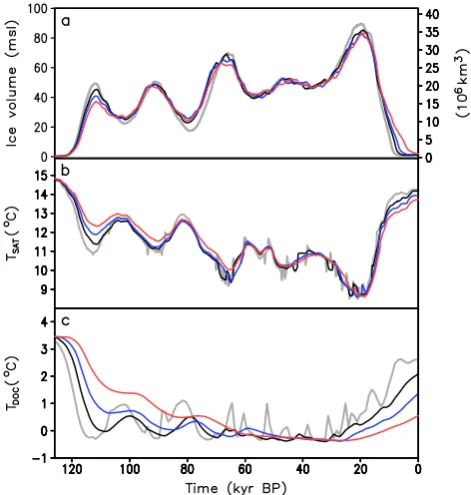
times faster than in reality, whereNis the acceleration factor. As a result, the exchange of information between the climate and the ice sheet model components occurs every year for the climate and eachNth year for the ice sheet component. Calov et al. (2009) showed that the climate component can be considerably accelerated without significant loss of accu-racy in simulation of the glacial inception. Here, we extend this analysis to the whole glacial cycle. Figure 12a shows the simulated global ice volume in three runs with acceler-ation factors of 5, 10 and 20 in comparison with the (fully synchronous) BE. With respect to simulated ice volume, the agreement between accelerated and BE remains reasonably good up to an acceleration factor of 20. The same is true for the globally averaged surface air temperature, although, pronounced millennial scale variability is already consider-ably suppressed for a two-fold acceleration (not shown). Fi-nally, the simulated deep water temperature is considerably affected by acceleration technique (Fig. 12c). Therefore, our experiments indicate that some aspects of glacial variability on orbital time scales can be successfully reproduced, even when using a large acceleration factor but considerable delay is introduced in the deep ocean evolution. The latter prob-lem can be at least partly mitigated by using an additional acceleration scheme for the deep ocean, as proposed by Liu et al. (2004).
6 Discussion and conclusions
Fig. 12. Effect of acceleration of the climate component on
simu-lated (a) NH ice volume, (b) global annual mean surface air temper-ature and (c) globally averaged deep ocean (4 km) tempertemper-ature. The grey lines in all figures show the Baseline Experiment. The black, blue and red lines indicate experiments with an acceleration by a factor of 5, 10 and 20, respectively.
interface. Compared to our previous work (C05), we addi-tionally introduced radiative forcing of atmospheric dust and the effect of deposition of dust produced by glacial erosion.
Our experiments demonstrate that the CLIMBER-2 model with an appropriate choice of model parameters simulates the major aspects of the last glacial cycle under orbital and greenhouse gases forcing rather realistically. In the simu-lations, the glacial cycle begins with a relatively abrupt lat-eral expansion of the North American ice sheets and parallel growth of the smaller northern European ice sheets. During the initial phase of the glacial cycle (MIS 5), the ice sheets experience large variations on precessional time scales. Later on, due to a decrease in the magnitude of the precessional cy-cle and a stabilising effect of low CO2concentration, the ice sheets remain large and grow consistently before reaching their maximum at around 20 kyr BP. The spatial extent of the simulated ice sheets at the LGM agrees reasonably well with palaeoclimate reconstructions. Only the thickness of the cen-tral part of Laurentide ice sheet is underestimated and Alaska appear to be glaciated too strongly. Simulated components of the mass balance are strongly affected by the ice volume and orbital forcing. Simulated total ablation is closely related to Milankovitch forcing, but leads it by several thousand years, while the total accumulation closely follows the area covered by the ice sheets.
lier by Peltier and Marshall (1995).
During the second part of the glacial cycle, the Laurentide ice sheet experienced large scale internal oscillations with a typical periodicity of about 6000 years, in many respects re-sembling observed Heinrich events. During the same period of time, glacial AMOC becomes unstable and experiences numerous transitions between different modes of operation, resulting in abrupt climate shifts over the North Atlantic realm resembling observed Dansgaard-Oeschger events. It is important to stress that the model simulates millennial scale climate variability without any explicit external forcing with the same periodicity. Millennial scale climate variability in our model is the results of internal instability of two com-ponents of the climate system: ice sheets and AMOC under glacial climate conditions.
Results from a set of sensitivity experiments demonstrate high sensitivity of simulated glacial cycle to the choice of some modelling parameters, and thus indicate the challenge to perform realistic simulations of glacial cycles with the computationally expensive models. At the same time, our results indicate that the computational cost of the simulation of the glacial cycle can be considerably reduced by using of the appropriate acceleration technique. At least as far as the simulated global ice volume is concerned, acceleration with a factor of up to 20 does not significantly disturb the simula-tion of the glacial cycle.
Appendix A
Parameterisation of dust deposition rate
The dust deposition rate in the model is computed as the sum of two components: the “background” dust deposition, con-stituted by the entrainment of dust from bare soilDb, and the
“glaciogenic” dustDg, originating from the glacial erosion at the periphery of the ice sheets. The first component, as in C05, is computed using results of the time slice simulation by Mahowald et al. (1999) for modern and LGM conditions. The dust deposition rate at each point and time is computed as a weighted sum of modern and LGM dust deposition rates, where the weight coefficient is proportional to the total NH ice volume:
where r=V /VLGM, V is the NH ice volume (in msl),
VLGM=100 msl is the NH ice volume at LGM, DLGM and
DMOD are dust deposition rates computed in Mahowald et al. (1999) for LGM and modern conditions respectively.
The deposition of the glaciogenic dust is computed us-ing a rather crude parameterisation based on the assumption that the glaciogenic source of dust is determined by the sed-iment transport through the margin of ice sheet. Namely, we assume that a certain fraction of the sediments accumu-lated in the ice-free grid cells neighbouring to the ice cov-ered grid cells becomes airborne and its transport in the at-mosphere can be described as a macroturbulent diffusion. It is naturally to assume that the production of glaciogenic dust is proportional to the sediment flux through the margin of the ice sheets. The later is related to the sliding velocity of the ice sheet in the proximity of the ice margin and the ad-vance/retreat velocity of the ice sheet margin. To overcome numerical problems related to fluctuations in simulated val-ues of both velocities, we introduced a new characteristics, the thickness of the “sediment excess”He, which represents
time-integrated convergence of the sediment transport by the ice sheets. The corresponding equation forHeis written as
dHe
dt = −
∂
∂x(uHa)−
∂
∂y(vHa)−E, (A2)
with the additional constraintHe≥0. Here, (u,v) is the
slid-ing velocity of the ice sheets, which is also assumed to be the velocity of the upper layer of sediments,Hais the
thick-ness of the active (water saturated) sediment layer, i.e. the unconsolidated layer of sediments which is moved by the ice sheet. The value ofHa is set to 0.1 m for rocks and 1 m for
continental area covered by terrestrial sediments. By keeping
Haindependent of time, we assume that changes in the area
covered by terrestrial sediments can be neglected over one glacial cycle. This would not be an appropriate assumption for the simulation of the whole Quaternary.
The termEin Eq. (A2) represents the decay of accumu-lated “sediment excess” due to water and wind erosion. This term is only applied outside of the ice sheets and is expressed in the form
E=He
τ ,
where the characteristic time scale of erosionτ is set to 1000 years. Assuming a fixed fraction of wind erosion in the total erosion of the “sediment excess”, the emission of glaciogenic dust per unit of area is
Sg=kgE=kg He
τ , (A3)
where the values of the empirical parameterkg=105g/m3was
chosen to match reconstructed glaciogenic dust deposition rate given in Mahowald at al. (2006a). Parameterkghas the
units of density and its value implies that less than 10% of the sediments transported by the ice sheet become airborne.
Equation (A2) is formally solved over the whole continental area, but positive “sediment excess” is formed only in the grid cells along the margin of the ice sheets and these grid cells become the source of aeolian dust only if they are ice free.
Assuming an universal vertical profile of dust in the atmo-sphere, isotropic macroturbulent mixing of the aeolian dust with the constant diffusion coefficient K and the constant residence time of the dust in the atmosphereτa, the balance
equation for the total dust load in the atmospheric columnQ
(in g/m2)can be described by the equation
Sg+K1Q−
Q
τa=0, (A4)
where1is the Laplace operator and Qτ =Dgis the dust
de-position rate. Although Eq. (A4) is simple, solving it on the ice sheet model grid is computationally expensive. There-fore, we use instead an equivalent but less expensive ap-proach by computing the deposition rate of glaciogenic dust at any location (xo,yo)by integrating the emission of dust
due to glacial erosionSgover the surrounding area Dg(x0,y0)=
ZZ
Sg(x,y)f (l) dxdy, (A5)
wherel=p(x−x0)2+(y−y0)2and, due to conservation of mass, the universal functionf (l)must satisfy the condition
ZZ
f (l) dxdy=1.
The function f was obtained by solving Eq. (A4) numeri-cally for a singular dust source and usingK=2·106m2/s and
τa=5 days. The combination of these two parameters gives
the length scaleL= √
Kτ=106m, which represent the radius of influence of a singular dust source. Sincef (l)decrease rapidly with the distance from the source, the size of the in-tegration domaincan be chosen with sufficient accuracy on the order of the magnitude ofL.
To take into account the effect of elevated ice sheets on the dust transport towards the ice sheet interior, we imposed an additional reduction on the dust deposition over the ice sheet as a function of the distance from the ice sheet margin. The length scale for the dust deposition decay is set to 500 km.
Appendix B
Calculation of the equivalent CO2concentration
in such a way that it is 280 ppm for the preindustrial condi-tions and gives the right changes in the total radiative forcing for the concentrations of CO2, CH4and N2O different from preindustrial values:
1RECO2=1RCO2+1RCH4+1RN2O, (B1)
where1RECO2=5.35ln
Ce
Co
is the radiative forcing of the equivalent CO2 concentrationCe,1RCO2=5.35ln
C
Co
is the radiative forcing of the “real” CO2 concentration C, andCo=280 ppm is preindustrial CO2concentration. Radia-tive forcings of CH4,1RCH4, and N2O,1RN2O, were com-puted using corresponding formulas from the IPCC report (Houghton et al., 1996). All radiative forcings are relative to the preindustrial concentrations of corresponding GHGs. By substituting values of individual radiative forcings into Eq. (B1) we calculate the value of equivalent CO2 concen-tration, which then was used in model simulations. Note that by definition,Ce=Co for preindustrial climate conditions.
The concentrations of individual greenhouse gases were av-eraged over thousand years (in case the resolution of indi-vidual records was better than one thousand years). When computing equivalent CO2concentration, following Hansen et al. (2005), we took into account, the fact that the resulting radiative forcing of CH4is 40% higher than its pure radiative effect due to methane decomposition in the stratosphere and the production of additional water vapour.
Acknowledgements. We would like to thank Ralf Greve for
pro-viding us with the ice sheet model SICOPOLIS. The comments by three anonymous reviewers considerably improved the manuscript. This project was partly funded by the Deutsche Forschungsgemein-schaft CL 178/4-1 and CL 178/4-2.
Edited by: A. Paul
References
Abe-Ouchi, A., Segawa, T., and Saito, F.: Climatic Conditions for modelling the Northern Hemisphere ice sheets throughout the ice age cycle, Clim. Past, 3, 423–438, 2007,
http://www.clim-past.net/3/423/2007/.
Berger A.: Long-term variations of daily insolation and Quaternary climatic change, J. Atmos. Sci., 35, 2362–2367, 1978.
tion and climate dynamics in the Holocene: experiments with the CLIMBER-2 model, Global Biogeochem. Cy., 16, 1139, doi:10.1029/2001GB001662, 2002.
Calov, R. and Ganopolski, A.: Multistability and hysteresis in the climate-cryosphere system under orbital forcing, Geophys. Res. Lett., 32, L21717, doi:10.1029/2005GL024518, 2005.
Calov, R., Ganopolski, A., Petoukhov, V., Claussen, M., and Greve, R.: Large-scale instabilities of the Laurentide Ice Sheet simu-lated in a fully coupled climate-system model, Geophys. Res. Lett., 29, 2216, doi:10.1029/2002GL016078, 2002.
Calov, R., Ganopolski, A., Claussen, M., Petoukhov, V., and Greve. R.: Transient simulation of the last glacial inception. Part I: Glacial inception as a bifurcation of the climate system, Clim. Dynam., 24, 545–561, doi:10.1007/s00382-005-0007-6, 2005. Calov, R., Ganopolski, A., Kubatzki, C., and Claussen, M.:
Mech-anisms and time scales of glacial inception simulated with an Earth system model of intermediate complexity, Clim. Past, 5, 245–258, 2009,
http://www.clim-past.net/5/245/2009/.
Calov, R. and Hutter, K.: The thermomechanical response of the Greenland ice sheet to various climate scenarios, Clim. Dynam., 12, 243–260, 1996.
Charbit, S., Ritz, C., Philippon, G., Peyaud, V., and Kageyama, M.: Numerical reconstructions of the Northern Hemisphere ice sheets through the last glacial-interglacial cycle, Clim. Past, 3, 15–37, 2007,
http://www.clim-past.net/3/15/2007/.
Claquin, T., Roelandt, C., Kohfeld, K. E., Harrison, S. P., Tegen, I., Prentice, I. C., Balkanski, Y., Bergametti, G., Hansson, M., Mahowald, N., Rodhe, H., and Schulz, M.: Radiative forcing of climate by ice-age atmospheric dust, Clim. Dynam., 20, 193– 202, doi:10.1007/s00382-002-0269-1, 2003.
Claussen, M., Mysak, L. A., Weaver, A. J., Crucifix, M., Fichefet, T., Loutre, M.-F., Weber, S. L., Alcamo, J., Alexeev, V. A., Berger, A., Calov, R., Ganopolski, A., Goosse, H., Lohman, G., Lunkeit, F., Mokhov, I. I., Petoukhov, V., Stone, P., and Wang, Zh.: Earth system models of intermediate complexity: Closing the gap in the spectrum of climate system models, Clim. Dynam., 18, 579–586, 2002.
Crowley, T. J.: North Atlantic Deep Water cools the southern hemi-sphere, Paleoceanography, 7, 489–497, 1992.
Deblonde, G., Peltier, W. R., and Hyde, W. T.: Simulations of con-tinental ice sheet growth over the last glacial-interglacial cycle: experiments with a one level seasonal energy balance model in-cluding seasonal ice albedo feedback, Global Planet. Change, 6, 37–55, 1992.
Geo-phys. Res., 96, 13139–13161, 1991.
Ganopolski, A.: Glacial Integrative modelling, Philos. T. R. Soc. A, 361, 1871–1884, 2003.
Ganopolski, A. and Rahmstorf, S.: Rapid changes of glacial cli-mate simulated in a coupled clicli-mate model, Nature, 409, 153– 158, 2001.
Ganopolski, A. and Roche, D.: On the nature of leads and lags dur-ing glacial-interglacial transitions, Quaternary Sci. Rev., 37/38, 3361–3378, doi:10.1016/j.quascirev.2009.09.019, 2009. Greve, R.: A continuum-mechanical formulation for shallow
poly-thermal ice sheets, Philos. T. R. Soc. Lon. A, 355, 921–974, 1997.
Hansen, J., Sato, M., Ruedy, R., Nazarenko, L., Lacis, A., Schmidt, G. A., Russell, G., Aleinov, I., Bauer, M., Bauer, S., Bell, N., Cairns, B., Canuto, V., Chandler, M., Cheng, Y., Del Genio, A., Faluvegi, G., Fleming, E., Friend, A., Hall, T., Jackman, C., Kel-ley, M., Kiang, N., Koch, D., Lean, J., Lerner, J., Lo, K., Menon, S., Miller, R., Minnis, P., Novakov, T., Oinas, V., Perlwitz, J., Perlwitz, J., Rind, D., Romanou, A., Shindell, D., Stone, P., Sun, S., Tausnev, N., Thresher, D., Wielicki, B., Wong, T., Yao, M., and Zhang, S.: Efficacy of climate forcings, J. Geophys. Res., 110, D18104, doi:10.1029/2005JD005776, 2005.
Houghton, J. T., Meira Filho, L. G., Callender, B. A., Harris, N., Kattenberg, A., and Maskell, K.: Climate change 1995: the science of climate change. Contribution of WGI to the sec-ond assessment report of the intergovernmental panel on climate change, Cambridge University Press, New York, 572 pp., 1996. Huybrechts, P.: Sea-level changes at the LGM from ice-dynamics
reconstructions of the Greenland and Antarctic ice sheets during the glacial cycles, Quaternary Sci. Rev., 21, 203–231, 2002. Krinner, G., Boucher, O., and Balkanski, Y.: Ice-free glacial
north-ern Asia due to dust deposition on snow, Clim. Dynam., 27, 613– 625, doi:10.1007/s00382-006-0159-z, 2006.
Lambeck, K., Esat, T. M., and Potter, E. K.: Links between climate and sea levels for the past three million years, Nature, 419, 199– 206, 2002.
Laske, G. and Masters, G. A.: Global Digital Map of Sediment Thickness, EOS Trans. AGU, 78, F483, 1997.
Liu, Z., Lewis, W., and Ganopolski, A.: An acceleration scheme for the simulation of long term climate evolution, Clim. Dynam., 22, 771–781, 2004.
Lorenz, S. J. and, Lohmann, G: Acceleration technique for Mi-lankovitch type forcing in a coupled atmosphere-ocean circula-tion model: method and applicacircula-tion for the holocene, Clim. Dy-nam., 23, 727–743, 2004.
Loutre, M.-F. and Berger, A.: No glacial-interglacial cycle in the ice volume simulated under a constant astronomical forcing and a variable CO2, Geophys. Res. Lett., 27(6), 783–786, 2000.
Mahowald, N., Kohfeld, K. E., Hansson, M., Balkanski, Y., Har-rison, S. P., Prentice, I. C., Schulz, M., and Rodhe, H.: Dust sources and deposition during the last glacial maximum and cur-rent climate: A comparison of model results with paleodata from ice cores and marine sediments, J. Geophys. Res., 104, 15895– 15916, 1999.
Mahowald, N., Muhs, D. R, Levis, S., Rasch, P. J., Yoshioka, M., Zender, C. S., and Luo, C.: Change in atmospheric mineral aerosols in response to climate: Last glacial period, preindus-trial, modern, and doubled carbon dioxide climates, J. Geophys. Res., 111, D10202, doi:10.1029/2005JD006653, 2006a.
Mahowald, N., Yoshioka, M., Collins, W. D., Conley, A. J., Fill-more, D. W., and Coleman, D. B.: Climate response and radiative forcing from mineral aerosols during the last glacial maximum, pre-industrial, current and doubled-carbon dioxide climates, Geophys. Res. Lett., 33, L20705, doi:10.1029/2006GL026126, 2006b.
Marshall, S. J. and Clark, P. U.: Basal temperature evolution of North American ice sheets and implications for the 100-kyr cy-cle, Geophys. Res. Lett., 29, 2214, doi:10.1029/2002GL015192, 2002.
Paillard, D.: The timing of Pleistocene glaciations from a simple multiple-state climate model, Nature, 391, 378–381, 1998. Paillard, D.: Glacial cycles: Toward a new paradigm, Rev.
Geo-phys., 39, 325–346, 2001.
Paterson, W. S. B.: The physics of glaciers, Pergamon/Elsevier, Ox-ford, 1994.
Peltier, W. R.: Global glacial isostasy and the surface of the ice-age earth: The ice-5G (VM2) model and grace, Annu. Rev. Earth Pl. Sc., 32, 111–149, 2004.
Peltier, W. R. and Marshall, S. J.: Coupled energy-balance/ice-sheet model simulations of the glacial cycle: A possible con-nection between terminations and terrigenous dust, J. Geophys. Res., 100(D7), 14269–14289, 1995.
Petoukhov, V., Ganopolski, A., Brovkin, V., Claussen, M., Eliseev, A., Kubatzki, C., and Rahmstorf, S.: CLIMBER-2: A climate system model of intermediate complexity. Part I: Model descrip-tion and performance for present climate, Clim. Dynam., 16, 1– 17, 2000.
Pollard, D.: A simple ice-sheet model yields realistic 100 kyr glacial cycles, Nature, 296, 334–338, 1982.
Roche, D., Renssen, H., Weber, S.L., Goosse, H.: Could melt-water pulses have been sneaked unnoticed into the deep ocean during the last glacial?, Geophys. Res. Lett., 34, L24708, doi:10.1029/2007GL032064, 2007.
Schneider von Deimling, T., Held, H., Ganopolski, A., and Rahmstorf, S.: Climate sensitivity estimated from ensemble simulations of glacial climate, Clim. Dynam., 27, 149–163, doi:10.1007/s00382-006-0126-8, 2006.
Tarasov, L. and Peltier, W. R.: Terminating the 100 kyr ice age cycle, J. Geophys. Res., 102, 21665–21693, 1997.
Thompson, W. G. and Goldstein, S. L.: A radiometric calibra-tion of the SPECMAP timescale, supplementary data, Quaternay Sci. Rev., 25, 3207–3215, doi:10.1016/j.quascirev.2006.02.007, 2006.
Waelbroeck, C., Labeyrie, L., Michel. E., Duplessy, J. C., Mc-Manus, J. F., Lambeck, K., Balbon, E., and Labracherie, M.: Sea-level and deep water temperature changes derived from ben-thonic foraminifera isotopic records, Quaternary Sci. Rev., 21, 295–305, 2002.
Wang, Z. and Mysak, L. A.: Simulation of the last glacial inception and rapid ice sheet growth in the McGill Paleoclimate Model, Geophys. Res. Lett., 29, 2102, doi:10.1029/2002GL015120, 2002.
Warren, S. G. and Wiscombe, W. J.: A model for the spectral albedo of snow. II: snow containing atmospheric aerosol, J. Atmos. Sci., 37, 2734–2745, 1980.