Forced versus coupled dynamics in Earth system modelling and prediction

(1)

SRef-ID: 1607-7946/npg/2005-12-311 European Geosciences Union

Nonlinear Processes

in Geophysics

Forced versus coupled dynamics in Earth system modelling and

prediction

B. Knopf1, H. Held1, and H. J. Schellnhuber1,2

1_{Potsdam Institute for Climate Impact Research (PIK), P.O. Box 601203,14412 Potsdam, Germany} 2_{Tyndall Centre for Climate Change Research, Norwich, UK}

Received: 20 October 2004 – Revised: 10 February 2005 – Accepted: 11 February 2005 – Published: 17 February 2005

Abstract. We compare coupled nonlinear climate models and their simplified forced counterparts with respect to pre-dictability and phase space topology. Various types of uncer-tainty plague climate change simulation, which is, in turn, a crucial element of Earth System modelling. Since the cur-rently preferred strategy for simulating the climate system, or the Earth System at large, is the coupling of sub-system modules (representing, e.g. atmosphere, oceans, global vege-tation), this paper explicitly addresses the errors and indeter-minacies generated by the coupling procedure. The focus is on a comparison of forced dynamics as opposed to fully, i.e. intrinsically, coupled dynamics. The former represents a par-ticular type of simulation, where the time behaviour of one complex systems component is prescribed by data or some other external information source. Such a simplifying tech-nique is often employed in Earth System models in order to save computing resources, in particular when massive model inter-comparisons need to be carried out. Our contribution to the debate is based on the investigation of two representa-tive model examples, namely (i) a low-dimensional coupled atmosphere-ocean simulator, and (ii) a replica-like simulator embracing corresponding components.

Whereas in general the forced version (ii) is able to mimic its fully coupled counterpart (i), we show in this paper that for a considerable fraction of parameter- and state-space, the two approaches qualitatively differ. Here we take up a phenomenon concerning the predictability of coupled versus forced models that was reported earlier in this journal: the observation that the time series of the forced version display artificial predictive skill. We present an explanation in terms of nonlinear dynamical theory. In particular we observe an intermittent version of artificial predictive skill, which we call on-off synchronization, and trace it back to the appear-ance of unstable periodic orbits. We also find it to be gov-erned by a scaling law that allows us to estimate the proba-bility of artificial predictive skill. In addition to artificial pre-Correspondence to: B. Knopf

([email protected])

dictability we observe artificial bistability for the forced ver-sion, which has not been reported so far. The results suggest that bistability and intermittent predictability, when found in a forced model set-up, should always be cross-validated with alternative coupling designs before being taken for granted.

1 Introduction

In the climate modelling community it is common practice to establish a modular structure, consisting of ecosphere, bio-sphere, vegetation, ocean, atmobio-sphere, etc., that builds up an Earth System Model (cf. the Climate System Model project CSM Boville and Gent, 1998). Some of these components are also modelled by external forcing, described from ob-served data. This is done e.g. in the Atmospheric Model Intercomparison Project AMIP (Gates et al., 1992), where an atmospheric general circulation model (AGCM) is con-strained by realistic sea surface temperature and sea ice and the output is used for diagnostic research. Although this ex-periment is not meant to be used for climate change predic-tions, diagnostic subprojects have been established, though it is not quite clear to what extent the forced AGCM output is comparable to the system with complex ocean-atmosphere feedbacks. These coupled systems are investigated e.g. in the Coupled Model Intercomparison Project CMIP (Meehl et al., 2000; Covey et al., 2003a). The comparison of coupled ocean-atmosphere models with simulations using prescribed sea surface temperatures shows that there are indeed some important differences concerning e.g. temperatures near the pole and tropical precipitation (Covey et al., 2003b). Other publications mention a strong effect of the coupling on the midlatitude variability of the ocean-atmosphere system (Bar-sugli and Battisti, 1998) or on the decadal variability of oceanic variables in the North Pacific (Pierce et al., 2001).

(2)

po-tential constraints preventing the consistency of forcing and coupling. With this paper we want to emphasize that when forcing one module by another instead of coupling the two components, one has to keep in mind that inherently nonlin-ear phenomena can occur that lead to qualitatively different features than expected. This type of analysis that we are un-dertaking can be assigned to many other cases of investigat-ing forced versus coupled model runs.

For our study we use a conceptual model which, com-pared to more sophisticated climate models like GCMs, has the advantage that the model itself as well as the output can transparently be analysed along the lines of dynamical sys-tems’ theory. This makes it easier to realise path continua-tion of solucontinua-tions in parameter space. The results presented in this paper reveal the underlying mechanisms for certain artificial phenomena produced in forced systems. From the knowledge of the mechanism we then conclude that those shortfalls of forced models are generic. Therefore we do not so much suggest to perform path continuation for GCMs as well (although it has successfully been implemented also for GCMs (Dijkstra, 2000)) but we understand the following chapters as a motivation to cross-validate a certain class of forced GCM results by alternative coupling designs in quite a classical manner.

The structure of the paper is as follows: The coupled ocean-atmosphere model we are analysing is described in section 2 and the phenomenon of locking for coupled and forced trajectories is presented. In section 3 the mathemati-cal background for replica systems is introduced. In section 4 we analyse the model in dependence on its parameters and highlight some fundamental differences between forcing and coupling. The role of unstable periodic orbits concerning the locking phenomenon is also investigated. In section 5 we de-termine the statistics of the locking and deduce a power law scaling for the length of the locking phases. The paper will finish with the conclusions in section 6.

2 Coupled and forced model

To investigate the difference between a forced and a fully coupled set-up, a coupled atmosphere-ocean system is cho-sen because the predictability of the Earth’s climate de-pends strongly on the variability induced by the interaction of these two components. As a very instructive example of the coupled atmosphere-ocean system, the following low-order model is examined:

"!#$&%&%

(1)

'()*+,*.-/012(354

(2)

*(06+789-/563;:

(3)

4<=>:8@?

(4)

:6=A4'B?

(5)

withBDCFEHGIJ

,KMLFENJ

,+ODCFENJ

,-PMQ

,3RM?RSCFEHG

,

2(CFENTJ

,#UVGWCYX"LZJ ENTJ

,=([!#AX"Q

, where#

is a scaling factor with one unit of system’s time referring to 10 days.

68 69 70 71 72 73 74 75 76 77 78

−0.5 0 0.5 1 1.5

Fully coupled run

x

68 69 70 71 72 73 74 75 76 77 78

−0.5 0 0.5 1 1.5

time / yr Forced run

x

Fig. 1. Comparison of the fully coupled system (top) and the forced

system (bottom). A fully coupled run is taken as reference trajec-tory. Additional to the reference trajectory, in each subfigure there are runs from slightly varying initial conditions in atmospheric co-ordinates. In the upper figure the curves are from a fully coupled run. In the lower figure, the trajectories are forced by the ocean from the reference trajectory. In this figure, we have reproduced a major finding by Wittenberg and Anderson (1998).

This model is taken from Wittenberg and Anderson (1998). The atmosphere system model (Eq.(1)-(3)) is a potentially chaotic Lorenz system (Lorenz, 1984), that de-scribes the midlatitude quasi-geostrophic flow. While$

rep-resents the time, the variable

represents the intensity of the westerly wind current or the meridional temperature gradi-ent. The variables

and

are the amplitudes of the sine and cosine components of a large travelling wave, which trans-ports heat poleward.

and 2

are forcing terms based on the average north-south temperature contrast and the earth-sea temperature contrast, where the earth-seasonal variation of

is expressed through the sine. The ocean system is a sim-ple harmonic oscillator, with an oscillation frequency=

of four years, where p and q represent zonal asymmetries in sea surface temperature. The coupling between ocean and atmo-sphere proceeds through the interaction of these asymmetries with the model atmosphere’s eddy field (y and z).

Wittenberg and Anderson (1998) carried out two different sets of simulations. One set of simulations represents the outcome of the fully coupled system with little variation in the initial state vectors. In the other set the output of the ocean from one special run is used to force the atmosphere. Again this is undertaken for slightly perturbed initial condi-tions. So there are two ensembles: one from a fully coupled system and one from a forced system that includes no feed-back from the atmosphere to the ocean.

As can be seen from Fig. 1, which was reproduced from Wittenberg and Anderson (1998), the forced ensemble is more compact, but does not mirror the true solution. Further-more, Wittenberg and Anderson (1998) show that the

statis-Fig. 1. Comparison of the fully coupled system (top) and the forced system (bottom). A fully coupled run is taken as reference trajectory. Additional to the reference trajectory, in each subfigure there are runs from slightly varying initial conditions in atmospheric coordinates. In the upper figure the curves are from a fully coupled run. In the lower figure, the trajectories are forced by the ocean from the reference trajectory. In this figure, we have reproduced a major finding by Wittenberg and Anderson (1998).

tential constraints preventing the consistency of forcing and coupling. With this paper we want to emphasize that when forcing one module by another instead of coupling the two components, one has to keep in mind that inherently nonlin-ear phenomena can occur that lead to qualitatively different features than expected. This type of analysis that we are un-dertaking can be assigned to many other cases of investigat-ing forced versus coupled model runs.

For our study we use a conceptual model which, compared to more sophisticated climate models like GCMs, has the ad-vantage that the model itself as well as the output can trans-parently be analysed along the lines of dynamical systems’ theory. This makes it easier to realise path continuation of solutions in parameter space. The results presented in this paper reveal the underlying mechanisms for certain artificial phenomena produced in forced systems.

From the knowledge of the mechanism we then conclude that those shortfalls of forced models are generic. There-fore we do not so much suggest to perform path continuation for GCMs as well (although it has successfully been imple-mented also for GCMs, Dijkstra, 2000) but we understand the following sections as a motivation to cross-validate a cer-tain class of forced GCM results by alternative coupling de-signs in quite a classical manner.

The structure of the paper is as follows: The coupled ocean-atmosphere model we are analysing is described in Sect. 2 and the phenomenon of locking for coupled and forced trajectories is presented. In Sect. 3 the mathemati-cal background for replica systems is introduced. In Sect. 4 we analyse the model in dependence on its parameters and

highlight some fundamental differences between forcing and coupling. The role of unstable periodic orbits concerning the locking phenomenon is also investigated. In Sect. 5 we de-termine the statistics of the locking and deduce a power law scaling for the length of the locking phases. The paper will finish with the conclusions in Sect. 6.

2 Coupled and forced model

To investigate the difference between a forced and a fully coupled set-up, a coupled atmosphere-ocean system is cho-sen because the predictability of the Earth’s climate de-pends strongly on the variability induced by the interaction of these two components. As a very instructive example of the coupled atmosphere-ocean system, the following low-order model is examined:

˙

x = −y2−z2−ax+a(F+sin(2π γ t )) (1) ˙

y =xy−cy−bxz+G+αp (2) ˙

z=xz−cz+bxy+αq (3) ˙

p= −ωq−βy (4)

˙

q =ωp−βz (5)

with a=0.125, F=3.5, c=0.5, b=4, α=β=0.1, G=0.25,

γ=10/365.25,ω=2π γ /4, whereγ is a scaling factor with one unit of system’s time referring to 10 days.

This model is taken from Wittenberg and Anderson (1998). The atmosphere system model (Eqs. 1–3) is a poten-tially chaotic Lorenz system (Lorenz, 1984), that describes the midlatitude quasi-geostrophic flow. While t represents the time, the variablexrepresents the intensity of the west-erly wind current or the meridional temperature gradient. The variables y and z are the amplitudes of the sine and cosine components of a large travelling wave, which trans-ports heat poleward. F andG are forcing terms based on the average north-south temperature contrast and the earth-sea temperature contrast, where the earth-seasonal variation ofF

is expressed through the sine. The ocean system is a sim-ple harmonic oscillator, with an oscillation frequencyω of four years, where p and q represent zonal asymmetries in sea surface temperature. The coupling between ocean and atmo-sphere proceeds through the interaction of these asymmetries with the model atmosphere’s eddy field (y and z).

Wittenberg and Anderson (1998) carried out two different sets of simulations. One set of simulations represents the outcome of the fully coupled system with little variation in the initial state vectors. In the other set the output of the ocean from one special run is used to force the atmosphere. Again this is undertaken for slightly perturbed initial condi-tions. So there are two ensembles: one from a fully coupled system and one from a forced system that includes no feed-back from the atmosphere to the ocean.

(3)

statis-B. Knopf et al.: Forced versus coupled dynamics 313 tics of the forced variability, like spatial and temporal

dis-tributions, are significantly different from those of coupled variability. For modelling issues this means that a prescribed forcing (e.g. prescribing the sea surface temperature) cannot emulate the fully coupled system. The interesting effect of the forcing is that all trajectories sometimes lock on the true solution for a short time and then separate again, so partial synchronization, so called “locking” can be observed. One can conclude from this that on the one hand fully coupled and forced systems do not show the same behaviour but on the other hand that in truly forced systems there may exist a region in phase space, where predictability is very high. The question to be followed is what mechanism is responsible for the locking phenomenon and what types of coupling show such behaviour.

3 Mathematical framework

In order to explain the locking phenomenon, a stability anal-ysis of the system appears the most natural approach. In the tradition of Wittenberg and Anderson (1998) and Smith et al. (1999), one would expect that the local linear stability prop-erties govern the observed phenomenon. Empirically, how-ever, we find that the explanation for locking given in Wit-tenberg and Anderson (1998) does not hold. We find that locking shows no correlation to the trajectory’s residence in the “locking region” identified in Wittenberg and Anderson (1998) and, in particular, that locking persists an order of magnitude longer than the trajectory resides in the locking region. Contrary to a local linear stability analysis, we will relate the locking period to extended invariant manifolds, emerging from the nonlinear dynamics of the system. This will allow us to introduce meaningful time-averaged charac-teristics. To frame a discussion of potential nonlinear causes of locking, we follow the concepts of Pecora and Carroll (1990) and Pecora et al. (1997). Different from Fig. 1, where we looked at a set of several forced trajectories, we investi-gate here just the fully coupled run and one forced run. The forced system can be written as a so-called replica system (Pikovsky et al., 2001), where a replica of one or more equa-tions is made. Together with Eqs. (1)–(5) we have a replica system of the following form:

˙

x0_{= −}_y02₋_z02₋_ax0₊

a(F +sin(2π γ t )) (6) ˙

y0₌_x0

y0−cy0−bx0z0+G+αp (7) ˙

z0₌_x0

z0−cz0+bx0y0+αq (8) ˙

p0_{= −}_ωq0₋_βy0 ₍₉₎ ˙

q0₌_ωp0₋

βz0, (10)

where the primed system x0=(x0, y0, z0, p0, q0)T is identical to the original fully coupled system x=(x, y, z, p, q)T ex-cept for slightly different initial conditions and the substi-tuted variablesp andq instead of p0 and q0, that emulate the forcing through prescribed data. In this systemp0 and

q0 have no influence on the dynamics of the other primed variables and are only introduced to allow for a closed

math-tics of the forced variability, like spatial and temporal

dis-tributions, are significantly different from those of coupled

variability. For modelling issues this means that a prescribed

forcing (e.g. prescribing the sea surface temperature) cannot

emulate the fully coupled system. The interesting effect of

the forcing is that all trajectories sometimes lock on the true

solution for a short time and then separate again, so partial

synchronization, so called locking can be observed. One can

conclude from this that on the one hand fully coupled and

forced systems do not show the same behaviour but on the

other hand that in truly forced systems there may exist a

re-gion in phase space, where predictability is very high. The

question to be followed is what mechanism is responsible for

the locking phenomenon and what types of coupling show

such behaviour.

3

Mathematical framework

In order to explain the locking phenomenon, a stability

anal-ysis of the system appears the most natural approach. In the

tradition of Wittenberg and Anderson (1998) and Smith et al.

(1999), one would expect that the local linear stability

prop-erties govern the observed phenomenon. Empirically,

how-ever, we find that the explanation for locking given in

Wit-tenberg and Anderson (1998) does not hold. We find that

locking shows no correlation to the trajectory’s residence in

the “locking region” identified in Wittenberg and Anderson

(1998) and, in particular, that locking persists an order of

magnitude longer than the trajectory resides in the locking

region. Contrary to a local linear stability analysis, we will

relate the locking period to extended invariant manifolds,

emerging from the nonlinear dynamics of the system. This

will allow us to introduce meaningful time-averaged

charac-teristics. To frame a discussion of potential nonlinear causes

of locking, we follow the concepts of Pecora and Carroll

(1990) and Pecora et al. (1997). Different from Fig. 1, where

we looked at a set of several forced trajectories, we

investi-gate here just the fully coupled run and one forced run. The

forced system can be written as a so-called replica system

(Pikovsky et al., 2001), where a replica of one or more

equa-tions is made. Together with Eqs. (1)-(5) we have a replica

system of the following form:

B

B "!#$&%&%

(6)

0( +, .-/ 2(354

(7)

( +7 -/ 3;:

(8)

4 =>: B?A

(9)

: =A4 @? E

(10)

where the primed system x

4 : %

is

identi-cal to the original fully coupled system x

4 :[%

except for slightly different initial conditions and the

substi-tuted variables

4

and

:

instead of

4

and

:

, that emulate the

forcing through prescribed data. In this system

4

and

:

have

no influence on the dynamics of the other primed variables

and are only introduced to allow for a closed mathematical

50 60 70 80 90 100

0 0.5 1 1.5 2 2.5

time / yr

norm of error vector |x−x’|

Fig. 2. Norm of the error vector

x

between the fully

coupled and the forced run; (

).

form. With this formalization “reality” - prescribed through

data - is being represented through a perfect model scenario

in the model-world.

In Fig. 2 the norm of the error vector

x

is

plotted. Sometimes the two systems synchronize but then

suddenly the system shows long-lasting bursts where the two

trajectories seem to evolve independently.

Generally, this type of coupling between two identical

sys-tems can be written as

x

F

x

%

x

F

x

%

K

x

%,E

(11)

where K is the coupling function.

By transforming Eq. (11) to the transversal coordinates

x

x and considering only small perturbations, so

that x

x and F

x

%

F

x

%

J

x

%7

x

%

the equation

can be approximated by

x

F

x

%

F

x

%

K

x

%

J

x

%

x

K

x

%

(12)

where J

x

%

is the Jacobian matrix of F evaluated on the

syn-chronization manifold. A linearisation of the function K

x

%

around zero, where we assume that K

0

%<

0 and neglect

higher order terms of x

, leads to

x

J

x

%

K

%

x

(13)

with

K

x

! ! ! !

x

"$# E

(14)

In our case, where we have linear coupling, the matrix

K

is

K

%& & & & ' C C6COC@C C C6C639C

C C6COC 3

C C6COC@C C C6COC@C (*) ) ) ) + E

(15)

To achieve complete synchronization, it is required that

for

$-,/.

, x

goes to zero. From the linearised equation

(13) one would expect that the two systems will synchronize

if the transverse Lyapunov exponents, that are the Lyapunov

Fig. 2. Norm of the error vectorδx=|x−x0|between the fully cou-pled and the forced run; (a=0.09).

ematical form. With this formalization “reality” – prescribed through data – is being represented through a perfect model scenario in the model-world.

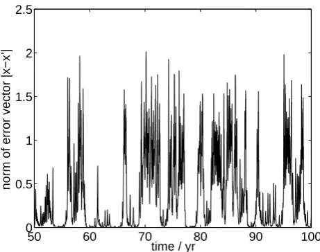
In Fig. 2 the norm of the error vectorδx=|x−x0_|_is plot-ted. Sometimes the two systems synchronize but then sud-denly the system shows long-lasting bursts, where the two trajectories seem to evolve independently.

Generally, this type of coupling between two identical sys-tems can be written as

˙

x=F(x) x˙0₌_F₍_x0

)+K(x−x0), (11) where K is the coupling function.

By transforming Eq. (11) to the transversal coordinates

x⊥=x−x0 and considering only small perturbations, so that

x≈x0and F(x0)≈F(x)+J(x)(x0−x)the equation can be ap-proximated by

˙

x⊥=F(x)−F(x0)−K(x⊥)≈J(x)x⊥−K(x⊥), (12) where J(x) is the Jacobian matrix of F evaluated on the synchronization manifold. A linearisation of the function

K(x)around zero, where we assume that K(0)=0 and neglect

higher order terms of x⊥, leads to ˙

x⊥≈(J(x)− ˜K)x⊥, (13)

with ˜ K=dK

dx

_x=0

. (14)

In our case, where we have linear coupling, the matrixK˜ is ˜ K=      

0 0 0 0 0 0 0 0α0 0 0 0 0α

0 0 0 0 0 0 0 0 0 0

(4)

exponents associated with Eq. (13), are all negative. This criterion was first proposed by Fujisaka and Yamada (1983), but in contrast to this, e.g. Gauthier and Bienfang (1996) observe only incomplete synchronization in their model in-stead of the proposed full synchronization, when the largest transverse Lyapunov exponent is smaller than zero. Several criteria for synchronization were developed (Blakely et al., 2000), but it was also shown there that for their model none of these criteria exactly predicts the range of the control pa-rameter where full synchronization can be observed.

In our case the largest transverse Lyapunov exponent is positive with

C5EC[Q

but we also observe partial syn-chronization. The time$

after which all information is lost and the two trajectories are totally independent, reads

$

G

;C%

(16)

where is the Lyapunov exponent,

denotes the character-istic length of the attractor and

C%

the error that cannot be dissolved by a given accuracy (Argyris et al., 1995). Here

$

is found to be about 1.3 years. Nevertheless locking can be observed over much longer timescales, as can be deduced from Fig. 2. This demonstrates that in the period of locking, a non-average, non-standard situation is present. Below we will link it to phase-space structures of low measure, yet of a noticeable domain of attraction.

4 Comparison of forced and coupled system

In this section we systematically compare the coupled to the forced system with respect to time-series properties as well as phase space topology. As a necessary condition for the forced system to emulate the coupled one in the time-domain we require that the forced system shows locking if and only if its coupled counterpart does.

4.1 System without seasonal cycle

An important structural difference between coupled and forced systems will be discussed in this chapter. In order to separate the two forcing effects in this model, namely the ocean forcing through the variables4

and:

and the seasonal forcing, the model is firstly investigated without the seasonal cycle. We analyse the dependence of the relative mean lock-ing time on the coupling strength 3

, see Fig. 3(a), where

$

(17)

where

is the length of the whole time series and$

is the time, where locking can be observed. This is averaged over many locking periods. Locking is defined by the norm of the error vector x

x x

of the two trajectories x and x being smaller than a critical threshold . For a propper

choice of see below, here we took CFECFG

.

A significant difference in the relative mean locking time for a fully coupled run and a forced run can be observed.

0.1 0.15 0.2 0.25 0.3 0.35 0.4 0.45 0.5 1E−6

1E−4 1E−2 1

<

τ

> / arb. units

0.1 0.15 0.2 0.25 0.3 0.35 0.4 0.45 0.5 0.96

0.98 1 1.02

x

stable periodic orbit unstable periodic orbit

0.1 0.15 0.2 0.25 0.3 0.35 0.4 0.45 0.5 0.94

0.96 0.98 1 1.02

coupling strength α

x

′

b.)

stable periodic orbit unstable periodic orbit c.)

a.)

Fig. 3. Relative mean locking time in relation to the most

domi-nant invariant sets (periodic orbits) for the system without seasonal

cycle (with ). (a) Relative mean locking time (see

Eq. 17) in dependence of the coupling strength! . For every point in this figure the initial conditions for x were chosen randomly and the trajectories were integrated over 500 years, according to 730500 time steps, after they settled down on an attractor. The forced trajec-tory was started on the attractor with slightly perturbed initial condi-tions, chosen from a gaussian distribution with a standard deviation of 0.01. For every value of the coupling strength! the integration was performed several times. As a mean length of zero cannot be depicted in a logarithmic plot, we added an offset of "$# ; (b) Bi-furcation diagram for the variable% of the five dimensional (5-D) driving system; for the periodic orbits, just one point referring to the maximum of the orbit is plotted; (c) Bifurcation diagram for the variable% of the 8-D combined drive and response system. A filled circle symbol represents a saddle node bifurcation, an unfilled circle stands for a torus bifurcation, an upward-pointing triangle denotes a period doubling bifurcation and a downward-pointing triangle sym-bolizes a branch point.

0.1 0.2 0.3 0.4 0.5

−1.5 −1 −0.5 0 0.5 1 1.5

x’

Fig. 4. Bifurcation diagram for% in dependence of the coupling

strength! in the system without seasonal cycle and .

The fully coupled system consists of two totally independent systems x and x , where the coupling matrix K of Eq. (15)

Fig. 3. Relative mean locking time in relation to the most dominant

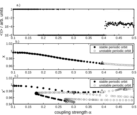
invariant sets (periodic orbits) for the system without seasonal cycle (witha=0.12). (a) Relative mean locking time<τ >(see Eq. 17) in dependence of the coupling strengthα. For every point in this figure the initial conditions for x were chosen randomly and the tra-jectories were integrated over 500 years, according to 730 500 time steps, after they settled down on an attractor. The forced trajectory was started on the attractor with slightly perturbed initial condi-tions, chosen from a gaussian distribution with a standard deviation of 0.01. For every value of the coupling strengthαthe integration was performed several times. As a mean length of zero cannot be depicted in a logarithmic plot, we added an offset of 10−6; (b) Bi-furcation diagram for the variablexof the five dimensional (5-D) driving system; for the periodic orbits, just one point referring to the maximum of the orbit is plotted; (c) Bifurcation diagram for the variablex0of the 8-D combined drive and response system. A filled circle symbol represents a saddle node bifurcation, an unfilled circle stands for a torus bifurcation, an upward-pointing triangle denotes a period doubling bifurcation and a downward-pointing triangle sym-bolizes a branch point.

To achieve complete synchronization, it is required that for t→∞, x⊥ goes to zero. From the linearised Eq. (13) one would expect that the two systems will synchronize if the transverse Lyapunov exponents, that are the Lyapunov exponents associated with Eq. (13), are all negative. This criterion was first proposed by Fujisaka and Yamada (1983), but in contrast to this, e.g. Gauthier and Bienfang (1996) ob-serve only incomplete synchronization in their model instead of the proposed full synchronization, when the largest trans-verse Lyapunov exponent is smaller than zero. Several crite-ria for synchronization were developed (Blakely et al., 2000), but it was also shown there that for their model none of these criteria exactly predicts the range of the control parameter, where full synchronization can be observed.

In our case the largest transverse Lyapunov exponent is positive withλ⊥≈0.084 but we also observe partial synchro-nization. The timet∗after which all information is lost and

the two trajectories are totally independent, reads

t∗≈ 1

λln L

δx(0), (16)

whereλis the Lyapunov exponent,Ldenotes the character-istic length of the attractor andδx(0)the error that cannot be dissolved by a given accuracy (Argyris et al., 1995). Here

t∗ is found to be about 1.3 years. Nevertheless locking can be observed over much longer timescales, as can be deduced from Fig. 2. This demonstrates that in the period of locking, a non-average, non-standard situation is present. Below we will link it to phase-space structures of low measure, yet of a noticeable domain of attraction.

4 Comparison of forced and coupled system

In this section we systematically compare the coupled to the forced system with respect to time-series properties as well as phase space topology. As a necessary condition for the forced system to emulate the coupled one in the time-domain we require that the forced system shows locking if and only if its coupled counterpart does.

4.1 System without seasonal cycle

An important structural difference between coupled and forced systems will be discussed in this section. In order to separate the two forcing effects in this model, namely the ocean forcing through the variablespandqand the seasonal forcing, the model is firstly investigated without the seasonal cycle. We analyse the dependence of the relative mean lock-ing time<τ >on the coupling strengthα, see Fig. 3a, where

τ = tlocking

T , (17)

whereT is the length of the whole time series andtlockingis

the time, where locking can be observed. This is averaged over many locking periods. Locking is defined by the norm of the error vectorδx=|x−x0|of the two trajectories x and

x0 being smaller than a critical threshold. For a propper choice ofsee below, here we took=0.01.

(5)

B. Knopf et al.: Forced versus coupled dynamics 315

exponents associated with Eq. (13), are all negative. This

criterion was first proposed by Fujisaka and Yamada (1983),

but in contrast to this, e.g. Gauthier and Bienfang (1996)

observe only incomplete synchronization in their model

in-stead of the proposed full synchronization, when the largest

transverse Lyapunov exponent is smaller than zero. Several

criteria for synchronization were developed (Blakely et al.,

2000), but it was also shown there that for their model none

of these criteria exactly predicts the range of the control

pa-rameter where full synchronization can be observed.

In our case the largest transverse Lyapunov exponent is

positive with

C5EC[Q

but we also observe partial

syn-chronization. The time

$

after which all information is lost

and the two trajectories are totally independent, reads

$

G

; C%

(16)

where

is the Lyapunov exponent,

denotes the

character-istic length of the attractor and

C%

the error that cannot be

dissolved by a given accuracy (Argyris et al., 1995). Here

$

is found to be about 1.3 years. Nevertheless locking can

be observed over much longer timescales, as can be deduced

from Fig. 2. This demonstrates that in the period of locking,

a non-average, non-standard situation is present. Below we

will link it to phase-space structures of low measure, yet of a

noticeable domain of attraction.

4

Comparison of forced and coupled system

In this section we systematically compare the coupled to the

forced system with respect to time-series properties as well

as phase space topology. As a necessary condition for the

forced system to emulate the coupled one in the time-domain

we require that the forced system shows locking if and only

if its coupled counterpart does.

4.1

System without seasonal cycle

An important structural difference between coupled and

forced systems will be discussed in this chapter. In order

to separate the two forcing effects in this model, namely the

ocean forcing through the variables

4

and

:

and the seasonal

forcing, the model is firstly investigated without the seasonal

cycle. We analyse the dependence of the relative mean

lock-ing time

on the coupling strength

3

, see Fig. 3(a),

where

$

(17)

where

is the length of the whole time series and

$

is

the time, where locking can be observed. This is averaged

over many locking periods. Locking is defined by the norm

of the error vector

x

of the two trajectories x

and x being smaller than a critical threshold

. For a propper

choice of

see below, here we took

CFECFG

.

A significant difference in the relative mean locking time

for a fully coupled run and a forced run can be observed.

0.1 0.15 0.2 0.25 0.3 0.35 0.4 0.45 0.5

1E−6 1E−4 1E−2 1

<

τ

> / arb. units

0.1 0.15 0.2 0.25 0.3 0.35 0.4 0.45 0.5

0.96 0.98 1 1.02

x

0.1 0.15 0.2 0.25 0.3 0.35 0.4 0.45 0.5

0.94 0.96 0.98 1 1.02

x

′

b.)

stable periodic orbit unstable periodic orbit c.)

a.)

Fig. 3. Relative mean locking time in relation to the most

domi-nant invariant sets (periodic orbits) for the system without seasonal cycle (with ). (a) Relative mean locking time (see

Eq. 17) in dependence of the coupling strength ! . For every point

in this figure the initial conditions for x were chosen randomly and the trajectories were integrated over 500 years, according to 730500 time steps, after they settled down on an attractor. The forced trajec-tory was started on the attractor with slightly perturbed initial condi-tions, chosen from a gaussian distribution with a standard deviation of 0.01. For every value of the coupling strength ! the integration

was performed several times. As a mean length of zero cannot be depicted in a logarithmic plot, we added an offset of "$# ; (b)

Bi-furcation diagram for the variable % of the five dimensional (5-D)

driving system; for the periodic orbits, just one point referring to the maximum of the orbit is plotted; (c) Bifurcation diagram for the variable%

of the 8-D combined drive and response system. A filled

circle symbol represents a saddle node bifurcation, an unfilled circle stands for a torus bifurcation, an upward-pointing triangle denotes a period doubling bifurcation and a downward-pointing triangle sym-bolizes a branch point.

0.1 0.2 0.3 0.4 0.5

−1.5 −1 −0.5 0 0.5 1 1.5

x’

Fig. 4. Bifurcation diagram for %

in dependence of the coupling

strength! in the system without seasonal cycle and .

The fully coupled system consists of two totally independent

systems x and x , where the coupling matrix K of Eq. (15)

Fig. 4. Bifurcation diagram forx0in dependence of the coupling strengthαin the system without seasonal cycle anda=0.12.

seasonal cycle. This suggests that the seasonal forcing is not the main cause of the observed intermittent behaviour.

The presented result does not depend on the choice of the threshold, provided that is not too small. The relative mean locking time<τ >grows only slowly with the, so there would be only a slight shift for the value of<τ >in Fig. 3a. On the other hand it is important to choose a thresh-oldthat is not too small (Lai, 1996), because it then takes a long time until the trajectory falls below the threshold and therefore one would need very long runs to calculate a reli-able value for the mean locking time<τ >.

In the remaining part of this section, we empirically corre-late time-series properties and phase-space topology in order to explain the locking phenomenon of the forced system. To get an impression of the phase space topology of the sys-tem in dependence of the parameterα, a bifurcation analysis is performed with the bifurcation analysis program AUTO (Doedel, 1981). In Fig. 3b the bifurcation diagram for the variablex of the fully coupled system – which simultaneu-osly plays the role of the forced system’s master trajectory – is plotted, in Fig. 3c the same is done for the variablex0

of the 8-D combined drive and response system. (Remember that for locking to occur,x andx0must coincide in the time series.) Forα<0.177, both diagrams display the identical bi-furcation diagram that simply consists of one stable periodic orbit. We propose that locking occurs in the forced system if both the master and the perturbed trajectory end up on the same periodic orbit.

Forα>0.177, the difference of the bifurcation diagrams is amazing: while for anyα<0.4 a stable periodic orbit exists in both the coupled (Fig. 3b) and the forced system (Fig. 3c), this orbit either lives on a different branch (forα∈[0.3,0.4]) or another stable periodic coexists (for α∈[0.177,0.277]), born in a saddle node bifurcation at α=0.177. In the lat-ter situation (α∈[0.177,0.277]), full synchronization can be observed if the perturbed trajectory starts in the domain of

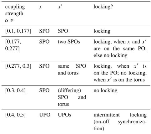
Table 1. Overview over the different regions in parameter space.

SPO stands for stable periodic orbit, UPO for unstable periodic or-bit.

coupling strength

α∈

x x0 locking?

[0.1, 0.177] SPO SPO locking

[0.177, 0.277]

SPO two SPOs locking, whenxandx0

are on the same PO; else no locking

[0.277, 0.3] SPO same SPO

and torus

locking, when x0 is

on the PO; no locking, whenx0is on the torus

[0.3, 0.4] SPO (differing)

SPO and

torus

no locking

[0.4, 0.5] UPO UPOs intermittent locking

(on-off

synchroniza-tion)

attraction of that periodic orbit which mimics the orbit of the master system (upper branch); otherwise the perturbed trajectory gets trapped by the concurring (lower branch) pe-riodic orbit and locking never occurs. In the former case (for

α∈[0.3,0.4]), the attracting orbits differ, hence synchroniza-tion should be impossible. This is in fact consistent with the relative mean locking time observed in Fig. 3a.

In Fig. 4 another bifurcation diagram for x0 is obtained by numerical integration to capture the movement on a torus, that cannot be depicted in the other diagram. In fact, the torus bifurcation is found in the upper Fig. 3c forα=0.277, but the torus cannot be followed with this method. For each pa-rameter valueαwe let the system settle down to an attractor and then plotted the forced variablex0, when the trajectory crosses they0axis at 0.5. From left to right we see again the stable periodic orbit and atα=0.177 the generation of a sec-ond orbit. From these stable periodic orbits a quasiperiodic motion on a torus emerges at α=0.277. The dynamics on the torus is sometimes adjourned by the stable periodic orbit that can be found in Fig. 3c forα<0.3. The torus disappears atα=0.4 through a period doubling bifurcation and passes into chaotic motion. For the driving system x no quasiperi-odic dynamics are found, so that forα∈[0.277,0.3], before the branch point atα=0.3 emerges, the system shows locking when x0is on the stable limit cycle or shows no locking when

x0 is on the torus. Which state will be adopted depends on the initial conditions. Forαlarger than the bifurcation value

(6)

note that synchronization effects might be artefacts from the

forced set-up.

In order to obtain a full understanding of the fundamental

discrepancies between the forced and fully coupled system,

in the following we will focus on the phenomenon of

inter-mittent synchronization that arises for

3

CFEQ

, where no

stable periodic orbit is detected.

4.2

The role of (un)stable periodic orbits

From the observations in the previous chapter we can

con-clude that if the system is in a region where it is on a stable

periodic orbit, the forced system shows locking all the time,

provided that we are in a region in parameter space where x

and x show the same bifurcation diagram. The

argumenta-tion reads as follows: as the orbit of the 8-D system is stable,

the trajectories of the driving system and the driven system

end up on the same periodic orbit, but they could still have a

phase shift. If there were a phase shift, then this shift would

also be seen in the ocean coordinates. But this is excluded

through the replica approach, where only the atmosphere

co-ordinates are varied. Contrary to this, for the coupled

sys-tem the ocean coordinates are also subject to the

perturba-tion, hence no synchronizing drive is present and no locking

will occur.

This emphasizes that full synchronization can in this case

be explained by a stable periodic orbit (or a stable

equilib-rium point) that drives the forced system to the same dynamic

behaviour.

After the stability has been lost in a bifurcation point, the

unstable periodic orbit embedded into the attractor influences

the system so that intermittently locking occurs even in a

region where the transversal Lyapunov exponent is positive

and – naively, “on average” – no synchronization is expected.

Therefore the concept of (unstable) periodic orbits seems to

be crucial for the locking phenomenon and the loss of

syn-chronization can be traced back to the transition from stable

to unstable periodic orbits. Ott and Sommerer (1994) call

this a nonhysteretic blowout bifurcation, where for

the system is on an attractor and for

on-off

intermit-tency can be detected. The role of unstable periodic orbits

(UPOs) for synchronization is also pointed out by Paz´o et al.

(2003) and by Pikovsky et al. (1997).

The interpretation with regard to UPOs can be stressed

through Fig. 5, where we analysed the phase space of the

locking regions in comparison to the full attracting set. It can

clearly be seen that the locking region is in good coincidence

with the unstable periodic orbit, whereas the non-locking

re-gion covers a much larger part of the whole phase space.

Just beyond a bifurcation point where a periodic orbit has

become unstable, the Monodromy matrix of the related

map-ping will display a long timescale on the unstable manifold,

and generically shorter time-scales for the remaining stable

manifold. Therefore, the unstable periodic orbit still has a

fair chance to attract on the stable manifold and synchronize

the trajectory. This will reveal itself as locking. After a while,

the long timescale on the unstable manifold manifests itself,

−0.4 −0.2 0 0.2 0.4 0.6 0.8 1 1.2 −1

−0.5 0 0.5 1 1.5

x

y

full attracting set (non−locking) unstable periodic orbit locking region 1 locking region 2

Fig. 5. Phase space of the full attracting set (non-locking region)

and of two exemplary locking regions (1 and 2), whereas here

re-gion refers to a period in time. For comparison the unstable periodic

orbit for this parameter constellation is plotted.

and the trajectory becomes repelled, reminiscent of

intermit-tency. Hence, we suggest that the intermittent locking can be

traced back to a co-existence of two identical unstable

peri-odic orbits, one in the fully coupled, and one in the combined

8D fully coupled and replica system.

In summary, there are two major differences in the coupled

and the forced system’s dynamics: first, the forced system

displays a richer bifurcation diagram including coexisting

stable invariant manifolds where the coupled system would

not (“artificial bistability”), and even if both the master and

the perturbed trajectory would end up on the same periodic

orbit, the coupled system lacks a synchronizer, hence cannot

display locking. At least the second effect is independent of

the complexity of the model and should occur in GCMs as

well.

One potential practical consequence could be within

weather forecast: if locking occurred already at the

begin-ning of the dynamics, in the “forecast period”, the

ensem-ble error along the trajectory could be vastly underestimated

in forced ensembles. This could imply that e.g., a hurricane

could affect a region on its way much earlier than anticipated.

Furthermore, artificial bistability could bring about that

climate policy becomes overly conservative as society tries

to prevent crossing a threshold which is just an artefact from

the forced model set-up.

4.3

System with seasonal cycle

The assertion of the role of stable and unstable periodic

or-bits can also be endorsed by Fig. 6, where the system with

seasonal cycle in dependence on the coupling strength

3

is

analysed. As before, the bifurcation diagram and the

rela-tive mean locking time are plotted. Again we can detect

in-termittent synchronization and it can be seen that there is a

transition from locking to intermittent locking.

Fig. 6 makes it clear that the presumption that with

stronger coupling the two systems will synchronize, is not

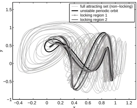
Fig. 5. Phase space of the full attracting set (non-locking region)

and of two exemplary locking regions (1 and 2), whereas here re-gion refers to a period in time. For comparison the unstable periodic orbit for this parameter constellation is plotted.

So far we can conclude that if the system is on the same stable periodic orbit for x and x0, we get full synchroniza-tion. On the other hand, when x runs on a periodic orbit not concurring to the replicate of x’s periodic orbit, locking cannot be observed. That means there can be intrinsic ob-stacles that a forced system performs as the fully coupled system. For modelling issues this is a crucial outcome, as for more sophisticated models the calculation of the state space of the forced and the coupled model is very costly so there is hardly any way to decide if forcing is suitable, above all because normally the fully coupled model is not known. For users of forced models is therefore of central importance to note that synchronization effects might be artefacts from the forced set-up.

In order to obtain a full understanding of the fundamen-tal discrepancies between the forced and fully coupled sys-tem, in the following we will focus on the phenomenon of intermittent synchronization that arises forα>0.4, where no stable periodic orbit is detected.

4.2 The role of (un)stable periodic orbits

From the observations in the previous section we can con-clude that if the system is in a region, where it is on a stable periodic orbit, the forced system shows locking all the time, provided that we are in a region in parameter space, where x and x0 show the same bifurcation diagram. The argumenta-tion reads as follows: as the orbit of the 8-D system is stable, the trajectories of the driving system and the driven system end up on the same periodic orbit, but they could still have a phase shift. If there were a phase shift, then this shift would also be seen in the ocean coordinates. But this is excluded through the replica approach, where only the atmosphere co-ordinates are varied. Contrary to this, for the coupled sys-tem the ocean coordinates are also subject to the

perturba-tion, hence no synchronizing drive is present and no locking will occur.

This emphasizes that full synchronization can in this case be explained by a stable periodic orbit (or a stable equilib-rium point) that drives the forced system to the same dynamic behaviour.

After the stability has been lost in a bifurcation point, the unstable periodic orbit embedded into the attractor influences the system so that intermittently locking occurs even in a re-gion, where the transversal Lyapunov exponent is positive and – naively, “on average” – no synchronization is expected. Therefore the concept of (unstable) periodic orbits seems to be crucial for the locking phenomenon and the loss of syn-chronization can be traced back to the transition from stable to unstable periodic orbits. Ott and Sommerer (1994) call this a “nonhysteretic” blowout bifurcation, where fora<ac

the system is on an attractor and for a>ac on-off

intermit-tency can be detected. The role of unstable periodic orbits (UPOs) for synchronization is also pointed out by Paz´o et al. (2003) and by Pikovsky et al. (1997).

The interpretation with regard to UPOs can be stressed through Fig. 5, where we analysed the phase space of the locking regions in comparison to the full attracting set. It can clearly be seen that the locking region is in good coincidence with the unstable periodic orbit, whereas the non-locking re-gion covers a much larger part of the whole phase space.

Just beyond a bifurcation point, where a periodic orbit has become unstable, the Monodromy matrix of the related map-ping will display a long timescale on the unstable manifold, and generically shorter time-scales for the remaining stable manifold. Therefore, the unstable periodic orbit still has a fair chance to attract on the stable manifold and synchronize the trajectory. This will reveal itself as locking. After a while, the long timescale on the unstable manifold manifests itself, and the trajectory becomes repelled, reminiscent of intermit-tency. Hence, we suggest that the intermittent locking can be traced back to a co-existence of two identical unstable peri-odic orbits, one in the fully coupled, and one in the combined 8D fully coupled and replica system.

In summary, there are two major differences in the coupled and the forced system’s dynamics: first, the forced system displays a richer bifurcation diagram including coexisting stable invariant manifolds, where the coupled system would not (“artificial bistability”), and even if both the master and the perturbed trajectory would end up on the same periodic orbit, the coupled system lacks a synchronizer, hence cannot display locking. At least the second effect is independent of the complexity of the model and should occur in GCMs as well.

(7)

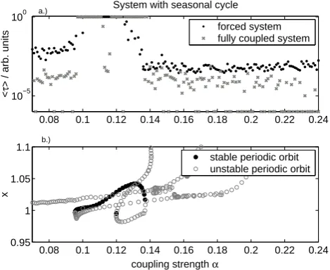
0.08 0.1 0.12 0.14 0.16 0.18 0.2 0.22 0.24

10−5

100

<

τ

> / arb. units

a.)

forced system fully coupled system

0.08 0.1 0.12 0.14 0.16 0.18 0.2 0.22 0.24

0.95 1 1.05 1.1

x

b.)

Fig. 6. Variation of the coupling strength! in the system with

sea-sonal cycle with . (a) Relative mean locking time

(see Eq. 17) in dependence on the coupling strength! . Again we

added an offset of " # to depict a mean length of zero; (b)

Bifur-cation diagram of the system. As for this parameter constellation

% and % show the same bifurcation diagram, just one bifurcation

diagram is plotted.

valid in this case. The system needs a stable manifold to be-come fully synchronized. For modelling issues, that means that it does not depend on the strength of coupling but on the state in the phase space if forcing can substitute coupling.

A significant difference to the situation without seasonal forcing is that here the fully coupled system shows lock-ing when the system is on a stable limit cycle, see Fig. 6(a), where the relative mean locking time is 1 in the locking re-gions, which means there is always locking. Intermittent syn-chronization can also sometimes be observed but less often than in the forced system (Fig. 6(a)). This is due to the sea-sonal forcing, that determines the frequency of the periodic orbit, so this locking bears on an external forcing and not on the intrinsic phenomenon of locking through prescribed forcing by variables. But as the seasonal cycle is also a kind of forcing, the chance of locking through an additional “syn-chronizer” increases.

4.4 Influence of the type of coupling

The system analysed so far is a system with linear coupling. As this is a very special case of coupling that is not often used in truly coupled models, we analyse a system without a seasonal cycle and with a nonlinear coupling to determine the influence of the type of coupling. The coupling has the following form:

O(5*.+,-,)823)4W

(18)

()6+71 -/563;: E

(19)

instead of Eqs. (2) and (3). As4

and:

vary approximately between -1 and 1, the introduced term bears strong nonlin-earity.

0.12 0.14 0.16 0.18 0.2 0.22

0.6 0.8 1 1.2 parameter a x, x’

0.12 0.14 0.16 0.18 0.2 0.22

10−4 10−2 100

system with nonlinear coupling (without seasonal cycle)

<

τ

> / arb. units

a.)

b.)

Fig. 7. Influence of the parameter in the system without seasonal

cycle and with nonlinear coupling as described through Eqs. (18) and (19). (a) Relative mean locking time (see Eq. 17) in dependence of the parameter ; (b) Bifurcation diagram of the

5-D and the 8-5-D system. Here% and% show the same bifurcation

diagram. The unfilled cycle stands for a torus bifurcation.

Instead of analysing the influence of the coupling strength

3

, here we focus on the effect of varying the parameter

. Again we have full locking when the system in on the same stable limit cycle for

and

, and transitions to intermittent locking when an UPO is reached, see Fig. 7. By varying the coupling strength3

in a range from 0.0 to 0.65 we discover a region of artificial bistability for

(not shown here) as we have seen before in the system with linear coupling (Fig. 3).

So all features found in the linear coupled system can also be discovered in the system with nonlinear coupling. This demonstrates that the type of coupling (linear or nonlinear) has no decisive influence on the locking phenomenon. Quite the contrary, as periodic orbits appear frequently in nonlin-ear systems, locking may occur generically in forced systems and is much less likely in their fully coupled counterparts. This stresses that for the locking phenomenon a linear stabil-ity analysis does not hold.

5 On-off Synchronization

The alternation between regions, where the error between the forced and coupled trajectory is nearly zero, and between re-gions with large bursts as shown in Fig. 2, resemble those of on-off intermittency. On-off intermittency, as introduced by Platt et al. (1993), refers to a situation where the variables of a chaotic dynamical system exhibit two distinct states where at the “off” state the system is nearly constant on an invariant manifold, and at the “on” state large bursts from these lami-nar phases occur. The frequency of bursts is controlled by a characteristic parameter4

of the system and approaches zero, when the so-called blowout bifurcation (Ott and Sommerer, 1994) is reached as4

attains a critical value4

. To assign

Fig. 6. Variation of the coupling strengthαin the system with sea-sonal cycle witha=0.27. (a) Relative mean locking time<τ >(see Eq. 17) in dependence on the coupling strengthα. Again we added an offset of 10−6to depict a mean length of zero; (b) Bifurcation diagram of the system. As for this parameter constellationxandx0 show the same bifurcation diagram, just one bifurcation diagram is plotted.

to prevent crossing a threshold which is just an artefact from the forced model set-up.

4.3 System with seasonal cycle

The assertion of the role of stable and unstable periodic or-bits can also be endorsed by Fig. 6, where the system with seasonal cycle in dependence on the coupling strengthαis analysed. As before, the bifurcation diagram and the rela-tive mean locking time are plotted. Again we can detect in-termittent synchronization and it can be seen that there is a transition from locking to intermittent locking.

Figure 6 makes it clear that the presumption that with stronger coupling the two systems will synchronize, is not valid in this case. The system needs a stable manifold to be-come fully synchronized. For modelling issues, that means that it does not depend on the strength of coupling but on the state in the phase space if forcing can substitute coupling.

A significant difference to the situation without seasonal forcing is that here the fully coupled system shows locking when the system is on a stable limit cycle, see Fig. 6a, where the relative mean locking time is 1 in the locking regions, which means there is always locking. Intermittent synchro-nization can also sometimes be observed but less often than in the forced system (Fig. 6a). This is due to the seasonal forcing, that determines the frequency of the periodic orbit, so this locking bears on an external forcing and not on the in-trinsic phenomenon of locking through prescribed forcing by variables. But as the seasonal cycle is also a kind of forcing, the chance of locking through an additional “synchronizer” increases.

0.08 0.1 0.12 0.14 0.16 0.18 0.2 0.22 0.24

10−5

100

<

τ

> / arb. units

a.)

forced system fully coupled system

0.08 0.1 0.12 0.14 0.16 0.18 0.2 0.22 0.24

0.95 1 1.05 1.1

x

b.)

Fig. 6. Variation of the coupling strength! in the system with

sea-sonal cycle with . (a) Relative mean locking time

(see Eq. 17) in dependence on the coupling strength! . Again we added an offset of " # to depict a mean length of zero; (b) Bifur-cation diagram of the system. As for this parameter constellation

% and%

show the same bifurcation diagram, just one bifurcation diagram is plotted.

valid in this case. The system needs a stable manifold to be-come fully synchronized. For modelling issues, that means that it does not depend on the strength of coupling but on the state in the phase space if forcing can substitute coupling.

A significant difference to the situation without seasonal forcing is that here the fully coupled system shows lock-ing when the system is on a stable limit cycle, see Fig. 6(a), where the relative mean locking time is 1 in the locking re-gions, which means there is always locking. Intermittent syn-chronization can also sometimes be observed but less often than in the forced system (Fig. 6(a)). This is due to the sea-sonal forcing, that determines the frequency of the periodic orbit, so this locking bears on an external forcing and not on the intrinsic phenomenon of locking through prescribed forcing by variables. But as the seasonal cycle is also a kind of forcing, the chance of locking through an additional “syn-chronizer” increases.

O(5*.+,-,)823)4W

(18)

()6+71 -/563;: E

(19)

instead of Eqs. (2) and (3). As4

and:

vary approximately between -1 and 1, the introduced term bears strong nonlin-earity.

0.12 0.14 0.16 0.18 0.2 0.22

0.6 0.8 1 1.2 parameter a x, x’

0.12 0.14 0.16 0.18 0.2 0.22

10−4 10−2 100

system with nonlinear coupling (without seasonal cycle)

<

τ

> / arb. units

a.)

b.)

Fig. 7. Influence of the parameter in the system without seasonal cycle and with nonlinear coupling as described through Eqs. (18)

and (19). (a) Relative mean locking time (see Eq. 17) in

dependence of the parameter ; (b) Bifurcation diagram of the

5-D and the 8-5-D system. Here% and% show the same bifurcation

diagram. The unfilled cycle stands for a torus bifurcation.

3

, here we focus on the effect of varying the parameter

. Again we have full locking when the system in on the same stable limit cycle for

and

, and transitions to intermittent locking when an UPO is reached, see Fig. 7. By varying the coupling strength3

in a range from 0.0 to 0.65 we discover a region of artificial bistability for

(not shown here) as we have seen before in the system with linear coupling (Fig. 3). So all features found in the linear coupled system can also be discovered in the system with nonlinear coupling. This demonstrates that the type of coupling (linear or nonlinear) has no decisive influence on the locking phenomenon. Quite the contrary, as periodic orbits appear frequently in nonlin-ear systems, locking may occur generically in forced systems and is much less likely in their fully coupled counterparts. This stresses that for the locking phenomenon a linear stabil-ity analysis does not hold.

5 On-off Synchronization

The alternation between regions, where the error between the forced and coupled trajectory is nearly zero, and between re-gions with large bursts as shown in Fig. 2, resemble those of on-off intermittency. On-off intermittency, as introduced by Platt et al. (1993), refers to a situation where the variables of a chaotic dynamical system exhibit two distinct states where at the “off” state the system is nearly constant on an invariant manifold, and at the “on” state large bursts from these lami-nar phases occur. The frequency of bursts is controlled by a characteristic parameter4

of the system and approaches zero, when the so-called blowout bifurcation (Ott and Sommerer, 1994) is reached as4

attains a critical value4

. To assign

Fig. 7. Influence of the parameterain the system without seasonal cycle and with nonlinear coupling as described through Eqs. (18) and (19). (a) Relative mean locking time<τ >(see Eq. 17) in de-pendence of the parametera; (b) Bifurcation diagram of the 5-D and the 8-D system. Herexandx0show the same bifurcation dia-gram. The unfilled cycle stands for a torus bifurcation.

˙

y =xy−cy−bxz+G+αp3x (18) ˙

z=xz−cz+bxy+αq3x. (19) instead of Eqs. (2) and (3). Aspandq vary approximately between−1 and 1, the introduced term bears strong nonlin-earity.

α, here we focus on the effect of varying the parametera. Again we have full locking when the system in on the same stable limit cycle forxandx0, and transitions to intermittent locking when an UPO is reached, see Fig. 7. By varying the coupling strengthαin a range from 0.0 to 0.65 we discover a region of artificial bistability forx0(not shown here) as we have seen before in the system with linear coupling (Fig. 3).

(8)

318 B. Knopf et al.: Forced versus coupled dynamics

−6 −4 −2 0 2 4

−12 −10 −8 −6 −4 −2 0 2

log(τ)

log p(

τ

)

B

A

slope: −3/2

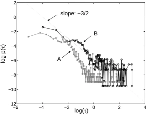
Fig. 8. Probability distribution of the length of the locking region

for more than 14,000 locking phases. Curve A is for a parameter

setting as given following Eq. 5 with

, for curve B the

parameter

is changed to 0.075, being closer to the bifurcation.

The dotted curve indicates a -3/2 power-law for comparison.

the phenomenon of on-off intermittency to our object of

in-terest, intermittency is not seen as laminar phases interrupted

by turbulent bursts but as locking of the fully coupled and

the forced trajectories (off-state) interrupted by non-locking

(on-state), which we will call on-off synchronization. The

transfer from on-off intermittency to on-off synchronization

becomes clearer when the difference between x and x is

un-derstood as a new variable.

Systems that generate on-off intermittency show

charac-teristic scaling laws for the intermittent phases (Heagy et al.,

1994; Lai, 1996), the distribution of the amplitudes of the

bursts and for the power spectrum of the trajectories (see

ref-erences cited by John et al. (2002)). Heagy et al. (1994)

in-vestigate a certain class of driven systems, that consists of a

discrete map and a random driving variable with a smooth

density. They show that for the probability distribution of the

length of the laminar phases

4

%

a power law holds with

4;

%

, where

is the length of the laminar phases

and

#

the scaling exponent that attains a universal value of

3/2 in the vicinity of the threshold for on-off intermittency.

This scaling law with the same exponent can also be

ap-proved for our case of on-off synchronization. The

proba-bility distribution

4

%

for the length of the locking region

for the parameter settings given in Fig. 1 (with

B CFEHGIJ

)

is plotted as curve A in Fig. 8. As the -3/2 power-law

dis-tribution is deduced theoretically exactly only for the critical

point

, we additionally plotted the probability distribution

for

CFEC[J

in curve B. This choice of the parameter is

very close to the bifurcation point from a stable to an

un-stable periodic orbit at

1 CFEC"L

, that was determined via

bifurcation analysis.

As both curves indicate, when the parameter

is close

to the bifurctation point the probability distribution obey

the predicted scaling law and differs from the exact relation

when the parameter is further away from the critical value.

For the very short locking phases both curves deviate from

the predicted dependence, because one approaches the time

scale of the simulation timestep. For the long locking phases

the distribution for curve A falls off exponentially, whereas

the two regions are connected by a shoulder, which is also

seen in other systems displaying on-off intermittency ((Platt

et al., 1993)). We assume that these imperfections from the

exact scaling law is in our case due to the distance of the

parameter

from the bifurcation point.

In this section we have shown that the scaling law for the

duration of the laminar phases in systems with on-off

inter-mittency also holds for a system with on-off synchronization

and could be extended to continuous systems with a

driv-ing system that is not random but chaotic. This means that

the power law scaling is more universal than proposed when

it was introduced. It can also be interpreted in this regard,

that the underlying mechanisms of on-off intermittency and

on-off synchronization are analogous. Intermittency is often

traced back to the “almost existence” of a stable periodic

or-bit, and in a similar way we discovered stable and unstable

periodic orbits as potential causes for locking.

The knowledge of the above power law does not only

stress the underlying nature of locking but will also help in

applications to estimate the relative importance of the

lock-ing phenomenon.

6

Conclusion

In this paper we consider the effect of module coupling on the

overall dynamical uncertainty for a paradigmatic non-linear

atmosphere-ocean system. We identify phase space as well

as time-series features with respect to which a forced model

set-up qualitatively differs from its fully coupled counterpart,

for systematic reasons. On the one hand, in accordance with

the general belief, the forced and the coupled model version

coincide in various main features, in particular in terms of

av-erage predictive skill and the existence of the same dominant

periodic orbit.

On the other hand, in fact we identify a considerable

frac-tion in parameter space for which the phase spaces of the two

model versions fundamentally differ: the phase space of the

fully coupled model is dominated by a single stable periodic

orbit, while the forced set-up allows for the existence of an

additional stable periodic orbit. Since this kind of

bistabil-ity is not found in the fully coupled model, which the forced

set-up is supposed to emulate, we call it “artificial

bistabil-ity”. These finding seems to contradict conventional

wis-dom in the Earth System modelling community stating that

a fully coupled model is more a complicated entity than a

forced derivate, hence the coupled version is expected to

dis-play more complicated features. However, in terms of replica

systems – a point of view we put forward in this paper – we

argue that in fact the forced set-up is the more complex one:

its dynamics are generated in an eight-dimensional

(ocean-dimension plus two times the atmosphere-(ocean-dimension) state

space, while that of the coupled version reside