www.clim-past.net/3/261/2007/
© Author(s) 2007. This work is licensed under a Creative Commons License.
Climate
of the Past
Results of PMIP2 coupled simulations of the Mid-Holocene and Last
Glacial Maximum – Part 1: experiments and large-scale features
P. Braconnot1, B. Otto-Bliesner2, S. Harrison3, S. Joussaume1, J.-Y. Peterchmitt1, A. Abe-Ouchi4, M. Crucifix5,6, E. Driesschaert6, Th. Fichefet6, C. D. Hewitt5, M. Kageyama1, A. Kitoh7, A. Laˆın´e1, M.-F. Loutre6, O. Marti1, U. Merkel8, G. Ramstein1, P. Valdes3, S. L. Weber9, Y. Yu10, and Y. Zhao3
1Laboratoire des Sciences du Climat et de l’Environnement, Unit´e mixte CEA-CNRS-UVSQ, Orme des Merisiers, bˆat 712,
91191 Gif-sur-Yvette Cedex, France
2National Center for Atmospheric Research, 1850 Table Mesa Drive, Boulder, Colorado, USA 3School of Geographical Sciences, University of Bristol, Bristol, BS8 1SS, UK
4Center for Climate System Research, The University of Tokyo, Japan 277-8568 and FRCGC/JAMSTEC, Yokohama
236-0001, Japan
5Met Office Hadley Centre, Fitzroy Road, Exeter EX1 3PB, UK
6Universit´e Catholique de Louvain, Institut d’Astronomie et de G´eophysique Georges Lemaˆıtre, B-1348 Louvain-la-Neuve,
Belgium
7Meteorological Research Institute, Tsukuba, Ibaraki 305-0052, Japan
8Universit¨at Bremen, FB5 Geosciences, Geosystem modelling, P.O. Box 330 440, 28334 Bremen, Germany 9Royal Netherlands Meteorological Institute, P.O. Box 201, 3730 AE De Bilt, The Netherlands
10LASG, Institute of Atmospheric Physics, Chinese Academy of Sciences, P.O. Box 9804, Beijing 100029, P. R. China
Received: 6 November 2006 – Published in Clim. Past Discuss.: 13 December 2006 Revised: 16 April 2007 – Accepted: 14 May 2007 – Published: 4 June 2007
Abstract. A set of coupled ocean-atmosphere simulations using state of the art climate models is now available for the Last Glacial Maximum and the Mid-Holocene through the second phase of the Paleoclimate Modeling Intercomparison Project (PMIP2). This study presents the large-scale features of the simulated climates and compares the new model re-sults to those of the atmospheric models from the first phase of the PMIP, for which sea surface temperature was pre-scribed or computed using simple slab ocean formulations. We consider the large-scale features of the climate change, pointing out some of the major differences between the dif-ferent sets of experiments. We show in particular that sys-tematic differences between PMIP1 and PMIP2 simulations are due to the interactive ocean, such as the amplification of the African monsoon at the Mid-Holocene or the change in precipitation in mid-latitudes at the LGM. Also the PMIP2 simulations are in general in better agreement with data than PMIP1 simulations.
Correspondence to: P. Braconnot
(pascale.braconnot@cea.fr)
1 Introduction
There is widespread concern about ongoing and future global environmental changes. Projections of possible future cli-mate changes, under different assumptions, can only be made with numerical models of the earth system. The IPCC re-ports (see IPCC, 2001) state that our confidence in the ability of models to project future climate has increased. Yet there are still significant discrepancies between different model re-sults, both in terms of simulated climate changes and more fundamental aspects of the representation of internal pro-cesses and feedbacks. We therefore need to be able to evalu-ate whether the model results are reliable, and also to attempt to estimate whether the models incorporate the required level of complexity to represent the range of possible responses of the coupled Earth system.
262 P. Braconnot et al.: New results from PMIP2 – Part 1: experiments and large-scale features comparisons of data and model results of the Paleoclimate
Modelling Intercomparison Project (PMIP) for key times in the past have provided grounds for confidence in some aspects of the models, while continuing to present impor-tant challenges (Joussaume and Taylor, 1995; PMIP, 2000). PMIP is a long-standing initiative endorsed by the World Cli-mate Research Programme (WCRP; JSC/CLIVAR working group on Coupled Models) and the International Geosphere and Biosphere Programme (IGBP; PAGES). The major goals of PMIP are to determine the ability of models to reproduce climate states that are different from those of today and to in-crease our understanding of climate change (Joussaume and Taylor, 1995).
In its initial phase (PMIP1), PMIP was designed to test the atmospheric component of climate models (atmospheric general circulation models: AGCMs), under the Last Glacial Maximum (LGM: ca. 21 000 years before present, 21 ka) and the Mid-Holocene (MH: ca. 6000 years before present, 6 ka) conditions. The LGM simulation was conceived as an ex-periment to examine the climate response to the presence of large ice sheets, cold oceans and lowered greenhouse gas concentrations. The Mid-Holocene simulation was designed as an experiment to examine the climate response to a change in the seasonal and latitudinal distribution of incoming so-lar radiation (insolation) caused by known changes in orbital forcing (Berger, 1978).
Many features of the PMIP1 experiments, including global cooling at the LGM and the expansion of the northern hemi-sphere summer monsoons during the Mid-Holocene, are ro-bust in that they are both shown by all models and by palaeoenvironmental observations (PMIP, 2000). However, the magnitude of the response is very different for the dif-ferent models. AGCMs forced by CLIMAP (1981) recon-struction of LGM sea surface temperature (SST), for exam-ple, fail to produce the magnitude of glacial cooling in the tropics shown by palaeoenvironmental observations (Farrera et al., 1999; Pinot et al., 1999). However, although some of the atmosphere-mixed-layer ocean models produce tropi-cal cooling of the right magnitude, others produce no greater cooling than the AGCM simulations (Harrison, 2000). Simi-larly, the simulated latitudinal expansion of the African mon-soon at 6 ka BP by AGCMs is considerably smaller than shown by palaeoenvironmental observations: some models underestimate the precipitation required to sustain vegetation at 23◦N in the Sahara by 50% while others fail to produce an increase in precipitation this far north (Joussaume et al., 1999). The PMIP1 results formed a crucial part of the eval-uation of climate models in the Third Assessment Report of the Intergovernmental Panel on Climatic Change (McAvaney et al., 2001).
The state-of-the-art models now include dynamical repre-sentations of the global atmosphere, ocean, sea-ice, and land surface, and the interactions among these components. Com-plementary experiments, examining the role of the ocean and of the land surface in past climate changes have also been
carried out by several PMIP1 participating groups (Cane et al., 2006). These experiments demonstrated that the ocean and vegetation feedbacks were both required to simulate the regional patterns and magnitude of past climate changes cor-rectly. Coupled simulations also allow us to consider new questions such as the response of the thermohaline circula-tion (THC) to changes in the boundary condicircula-tions and the impact of this response on climate change, or the changes in interannual to multidecadal variability and the role of ocean and vegetation feedbacks in modulating these changes.
The second phase of the project (PMIP2) was launched in 2002 (Harrison et al., 2002). The LGM and the Mid-Holocene remain key benchmark periods for the project, for which respectively 6 and 9 modeling groups per-formed coupled ocean-atmosphere (OA) and/or coupled ocean-atmosphere-vegetation (OAV) simulations following the same protocol. The objective of this overview paper is to highlight the large-scale features of these simulations, and to compare the results with those of PMIP1 where possible, as well as with data syntheses that were widely used to as-sess the realism of model results in PMIP1. Several anal-yses have already considered the results of these new sim-ulations, considering the polar amplification of temperature (Masson-Delmotte et al., 2006), model evaluation over the North Atlantic ocean and Eurasia at the LGM (Kageyama et al., 2006), climate sensitivity (Crucifix, 2006), the glacial THC in the Atlantic ocean (Weber et al., 2007), and tropi-cal climate variability over west Africa (Zhao et al., 2007). Here we provide an overview of the PMIP2 results for the LGM and the Mid-Holocene, highlighting changes in global temperature, and in the hydrological cycle. We only consider large-scale indicators, and the evaluation of model results in the tropical regions, using benchmarking diagrams proposed in PMIP1 (Joussaume et al., 1999; Pinot et al., 1999). A second part (see Braconnot et al., 2007) investigates in more depth changes in the position of the ITCZ in the tropics, the role of the change in snow and sea-ice cover in mid and high latitudes, and discusses how the new simulations reproduce some feedbacks, such as the vegetation feedback, identified in previous studies.
Table 1. Boundary conditions, trace gazes and Earth’s orbital parameters as recommended by the PMIP2 project.
Ice Sheets Topography Coastlines CO2 CH4 NO2 Eccentricity Obliquity Angular precession
(ppmv) (ppbv) (ppbv) (◦) (◦)
0 ka Modern Modern 280 760 270 0.0167724 23.446 102.04
6 ka Same as 0K Same as 0K 280 650 270 0.018682 24.105 0.87
21 ka ICE-5G ICE-5G 185 350 200 0.018994 22.949 114.42
2 Simulations of the Mid-Holocene and Last Glacial Maximum
As for PMIP1, a strict protocol is provided to run the PMIP2 21 ka and 6 ka experiments (see http://pmip2.lsce.ipsl.fr/). It represents the best compromise between the need to ac-count for the different forcings and realistic boundary condi-tions that guarantee the relevant character of the model-data comparisons, and the pragmatic constraints imposed by the model structures and stability (Table 1).
2.1 Experimental protocol for the control simulation The reference (control) simulation (0 ka) is a pre-industrial (circa 1750 A.D.) type climate. The orbital parameters are prescribed to the reference values of 1950 A.D. (as done in PMIP1), and trace gases correspond to 1750 A.D. The differ-ence between 1750 and 1950 insolation induced by changes in the orbital parameters is negligible, which explains why we neglect this aspect. Slight differences in the solar forc-ing arise, however, from the changes in the solar constant. In the simulations presented here, these changes are smaller than the changes in insolation or in boundary conditions we investigate for the 6 ka and 21 ka periods in the past and are thus neglected. PMIP2 uses the same solar constant for PI, MH and LGM.
In simulations with the coupled ocean-atmosphere (OA) version of the models, vegetation is prescribed for most mod-els to the present day distribution of vegetation. This may potentially affect model-data comparisons, because the pre-scribed vegetation already accounts for land use. Note that the present day distribution of vegetation is model depen-dent, since each group uses its own reference. In addition depending on the land-surface scheme used in the OA mod-els vegetation is prescribed and the effect of vegetation on albedo, roughness length, and resistance to evaporation is either prescribed, or, in more sophisticated schemes, com-puted depending on plant functional types, and on the sea-sonal evolution of the leaf area index. In the coupled ocean-atmosphere-vegetation (OAV) simulations, vegetation is in-teractively computed by the model, as well as all the parame-ters (albedo, roughness length,...) needed to compute surface heat and water fluxes with the atmosphere. In the latter case vegetation represents natural vegetation, which means that
Figure 1.1
Fig. 1. Ice 5G ice sheet reconstruction (topography in m) for the LGM used as boundary condition in the PMIP2 simulations.
land use is not accounted for in these simulations. As a con-sequence, for a given model, the OA and OAV pre-industrial simulations produce slightly different climates.
2.2 Last Glacial Maximum (21 ka) simulations
264 P. Braconnot et al.: New results from PMIP2 – Part 1: experiments and large-scale features
Figure 1. 2. Fig. 2. Insolation (W/m
2)averaged over (a) the Northern
Hemi-sphere and (b) the Southern HemiHemi-sphere for present day (0 ka), Mid-Holocene (6 ka) and the difference between the two (6 ka– 0 ka). Note that the modern calendar was used to compute the monthly means for both time periods. The seasonal cycle has been duplicated to better highlight the change in insolation during January–February in both hemispheres.
The land-sea mask and topography are changed so as to correctly account for the ice sheets and the lowering of sea level. The ICE-5G global reconstruction of ice sheet to-pography was adopted (Peltier, 2004) (Table 1). Surface altitude in 21 ka experiments is calculated as 0 ka + (ICE-5G 21 ka–ICE-(ICE-5G 0 ka), where ICE-(ICE-5G 21 ka and ICE-(ICE-5G 0 ka are the reconstructions for 21 ka and the present, re-spectively. This ice sheet reconstruction (Fig. 1) is differ-ent from the one (Peltier, 1994) used for PMIP1 simulations. The Fennoscandian ice-sheet doesn’t not extend as far east-ward and is significantly higher, which influences the results in the Siberian sector (Kageyama et al., 2006). The Keewatin Dome west of Hudson Bay is 2–3 km higher in a broad area of central Canada which affects the planetary wave struc-ture in the North Pacific-North America-North Atlantic sec-tor (Otto-Bliesner et al., 2006). The land-sea mask should be modified to be consistent with the lower sea level, but the way to achieve this is model dependent.
The globally averaged salinity of the LGM ocean is im-posed to be the same as in the control simulation. This is not realistic, because the lower sea-level imposes a mean differ-ence of about 1 PSU in global salinity. Recent studies
sug-gest that such a mean shift on salinity has nearly no impact on density gradient in the ocean (Weaver et al., 1998). Also, this change in salinity may have been regionally distributed, which is difficult to properly infer from data. We thus de-cided to neglect it. Note however that some of the models, like CCSM, were initialised from a previous LGM simula-tion that takes into account the lower salinity. Furthermore the experimental protocol recommends that net accumulation of snow over the northern ice sheets is compensated for by a freshwater input over the Arctic and north of 40◦N in the Atlantic. This mimics iceberg melting and closes the fresh-water balance. Moreover, changes in the river flow compo-nents should be accounted for, following as much as possible data based references. However, this is not considered in most simulations and differences in the fresh water flux en-tering the ocean arise from inter-model differences in both the treatment of snow accumulation and river run-off (Weber et al., 2007).
The 21 ka simulation poses a major technical challenge to bring the ocean circulation into a glacial state. To do this from the pre-industrial control simulation would require sev-eral thousand years of simulation. This is not feasible with complex models, and thus some form of acceleration tech-nique or asynchronous-coupling of the fast atmosphere and slow ocean has to be employed to bring the model into a glacial state prior to running the LGM experiment. Several approaches have been suggested, but it is not clear which of these will produce the best results. Each of the modelling groups therefore uses its own “spin-up” technique to initial-ize and initiate the 21 ka simulation. Details on the imple-mentation of the PMIP2 protocol in the individual models can be found in the model references provided in Table 2. 2.3 Mid-Holocene (6 ka) simulations
Table 2. PMIP2 OA and OAV model characteristics and references. The last two columns indicate which time slices were performed for each model. The crosses stand for OA simulations and the circles for OAV simulations.
Resolution Model name as
specified in PMIP2 database
Atm Long×lat (levels)
Ocean Long×lat (levels)
Flux Adjustment
Reference for model 6 ka 21 ka
CCSM3 T42 (26) 1◦×1◦(40) None Otto-Bliesner (2006) x x
ECBilt-Clio T21 (3) 3×3 (20) Basin-mean Vries and Weber (2005) x
ECBilt-CLIO-VECODE
T21 (3) 3×3 (20) Renssen et al. (2005) xo
ECHAM5-MPIOM1 T31 (19) 1.875◦×0.84◦(40) None Roeckner et al. (2003), Marsland et al. (2003), Haak et al. (2003)
x
FGOALS-g1.0 2.8x2.8 (26) 1◦×1◦(33) None Yu et al. (2002),
Yu et al. (2004)
x x
FOAM R15 (18) 2.8◦×1.4◦(16) None Jacob et al. (2001) xo
HadCM3M2 3.75◦×2.5◦(19) 1.25◦×1.25◦(20) None Gordon et al. (2000) xo UBRIS-HadCM3M2 3.75◦×2.5◦(19) 1.25◦×1.25◦(20) None Gordon et al. (2000) xo IPSL-CM4-V1-MR 3.75◦×2.5◦(19) 2◦×0.5◦(31) None Marti et al. (2005) x x
MIROC3.2 T42 (20) 1.4◦×0.5◦(43) None K-1 Model Developers
(K-1-Model-Developers, 2004)
x x
MRI-CGCM2.3fa T42 (30) 2.5◦×0.5◦(23) Yes Yukimoto et al. (2006) x
MRI-CGCM2.3nfa T42 (30) 2.5o×0.5o(23) None Yukimoto et al. (2006) x
Table 3. Trend in surface air temperature estimate from the monthly values stored in the PMIP2 database and expressed in◦C/century. Values larger than 0.05◦C/century are in bold.
Tas: trend in◦C/century Model name as specified in PMIP2 database 0 ka 6 ka 21 ka
CCSM3 −0.012 −0.007 −0.010
ECBilt-Clio −0.025 −0.009
ECBilt-CLIO-VECODE : oa −0.007 0.003
ECBilt-CLIO-VECODE : oav −0.008 0.003
ECHAM5-MPIOM1 0.034 −3E-04
FGOALS-g1.0 −0.025 0.001 −0.116
FOAM: oa −0.061 −0.015
FOAM : oav −0.072 −0.072
HadCM3M2: oa −3E-04 0.032
HadCM3M2: oav 0.032 −0.008
UBRIS-HadCM3M2: oa −0.057 −0.057
UBRIS-HadCM3M2: oav −0.030 0.001
IPSL-CM4-V1-MR 0.019 −0.023 −0.039
MIROC3.2 6E-04 −0.022 −0.050
MRI-CGCM2.3fa −0.060 −0.057
MRI-CGCM2.3nfa 0.117 0.064
one used in the control simulations. The consequence is that changes that occur in autumn will be slightly underestimated with this modern calendar in the northern hemisphere and overestimated in the southern hemisphere. In particular, the change in insolation plotted in Fig. 2 is underestimated by
about 10 W/m2 in Autumn (September and October) in the northern hemisphere and overestimated by 15 W/m2 in the southern hemisphere.
266 P. Braconnot et al.: New results from PMIP2 – Part 1: experiments and large-scale features concentrations of the other trace gases (CO2 and N2O) are
kept as in the pre-industrial simulations (Table 1). Dust and other aerosols (volcanism) are not considered. A first set of simulations is run with the OA version of the models. In these simulations vegetation is the same as in the control simulation, in order to determine the response of the ocean-atmosphere system to the changes in solar forcing. Simu-lations where the dynamical part of the vegetation model is activated (OAV simulations) are branched off the OA simu-lations. The analysis of feedbacks due to vegetation changes is not straightforward because of the differences between the OA and OAV control simulation listed above. Therefore, the modelling groups are encouraged to run the OA 6 ka simu-lation prescribing the vegetation of the OAV pre-industrial simulation as it is done in Braconnot et al. (1999). In this case the OA and OAV 6 ka simulations share the same control simulation (OAV pre-industrial) and the difference between the OA and OAV 6 ka simulations allows to discuss the role of the vegetation feedback.
2.4 Models and database
For most of the modelling groups, the version of the CGCMs used for PMIP2 (Table 2) is identical to the version used for future climate change predictions. However, only IPSL-CM4-V1 and MIROC3.2 were run with exactly the same res-olution. The other groups either consider a slightly different version or lower resolution. All the atmospheric components of the OA and OAV models participating in the project ac-count for the effect of CO2and other trace gases in their
ra-diative codes. They also all include a sea ice model in the oceanic component. Table 2 indicates the state of the simu-lations for the two time periods and provides references for the different models used. More simulations have been per-formed but are still subject of quality assessments before be-ing uploaded into the database, and are therefore not consid-ered here. In addition Earth system models of intermediate complexity (EMICS) have been included because they offer the opportunity to make lots of sensitivity experiments to test several aspects of the climate system in a more efficient way than GCMs.
For each time period and experiment, the models are run long enough for the trends over the final 100 years to be small. The last 100 or 200 years of experiments are con-sidered for the analyses and are uploaded in the common database. Mean seasonal cycles were computed from 100 year averages. Results of the different simulations are stored in a common database hosted at LSCE on raid disks and the data is distributed through a Linux file server. Guidelines, file format convention, variable names and structures, and utili-ties are adopted in coordination with the Coupled Modelling Intercomparison Project (see http://www-lsce.cea.fr/pmip2). Table 3 shows the trends global annual mean 2 m air sur-face temperature computed from the monthly data provided by each modelling group in the database. Most simulations
are in near surface equilibrium, with trends in surface air temperature that do not exceed 0.02◦C/century. Four
mod-els (FOAM, UBRIS-HadCM3CM2 OA, and the two MRIs) exhibit drifts larger than 0.05◦C/century, suggesting that the energy balance is not fully closed in these models or that the simulations were not run long enough. This may affect some of the results. Note also that for a same model, the drift is different from one simulation to the other.
For comparison, we also present model results from the PMIP1 database. The corresponding model references can be found in Joussaume et al. (1999) for MH and Pinot et al. (1999) for LGM. The atmospheric models correspond to the previous generation of climate models. Therefore, for a given model name, the model version may be very different from the one used in the coupled OA or OAV models consid-ered in PMIP2. This is why we do not show model names for these simulations in the following. The PMIP1 simulations of 6 ka are atmosphere-only simulations (SSTf), for which sea surface temperatures (SSTs) are kept as they are in the modern climate and the only difference with 0 ka arises from the orbital parameters. For 21 ka, all simulations used the Peltier ICE-4G ice sheet, and imposed lower concentration of gases (200 ppm for CO2). In a first set of simulations, the
SSTs were prescribed to the CLIMAP (1981) reconstruction (SSTf), whereas in a second set SSTs were computed using a slab ocean model coupled to the atmospheric model (SSTc). Mean seasonal cycles were computed for a 10 year average.
3 Large-scale features of the simulated climate
3.1 Last Glacial Maximum
As expected from the presence of the Fennoscandian and Laurentide ice sheets in the Northern Hemisphere and the lower trace gases concentrations in the atmosphere, the LGM climate is characterised by a large surface cooling (Fig. 3a) with maximum cooling (about −30◦C) over the ice sheets in the Northern Hemisphere (NH). The ice sheet height and the associated large cooling alter the characteristics of the stationary waves, and contribute to the large cooling (−5 to−10◦C) downstream over the whole Eurasian continent (Fig. 3a). In the tropical regions the continental cooling is of smaller magnitude (−2 to−5◦C). This moderate cooling is also found in most places over the ocean in mid-latitudes and in the tropical regions. The cooling does not exceed−2◦C
in several parts of the subtropical oceans in the Pacific and in the Southern Hemisphere (SH) in the Atlantic and Indian oceans.
(
a) PMIP2 OA mean model
(
b) PMIP1 SSTf mean model
(
c) PMIP1 SSTc mean model
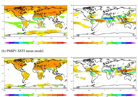
Figure 1.3:
Fig. 3. Annual mean LGM changes in temperature (◦C, left) and precipitation (mm/d, right) for (a) the ensemble mean of PMIP2 simulations, (b) the ensemble mean of PMIP1 simulations with fixed SST and (c) the ensemble mean of PMIP1 simulations with computed SST.
(Fig. 4a). Interestingly, model spread is largest in the south-ern hemisphere where the cooling varies from−2 to −5.3
◦C depending on the model (Fig. 4d). This is due to large
differences in the response of the circumpolar ocean and of
the temperature over sea-ice. The latter varies from a small cooling of−2◦C up to−10◦C when sea-ice cover increases
Masson-268 P. Braconnot et al.: New results from PMIP2 – Part 1: experiments and large-scale features
Figure 1.4 :
Fig. 4. Comparison of the change in surface air temperature (◦C) from PMIP1 OA, PMIP1 SSTf and PMIP1 SSTc experiments for (a) the global annual mean, (b) NH annual mean, (c) NH June-July-August-September (JJAS) and December-January-February (DJF) seasonal means, and (d) SH annual mean. The summer season (JJAS) is defined so as to cover the whole monsoon season in all climates.
Delmotte et al. (2006) report a−3.7 to−5.1◦C range, con-sistent with ice core estimates. In NH (Fig. 4b), the cooling is larger and model spread is smaller (2◦C). The seasonal contrast is small, with only a 1◦C difference in the magni-tude of the NH cooling between December-January-February (DJF) and June-July-August-September (JJAS), except for HadCM3M2 (Fig. 4c).
Tropical oceans were warmer in PMIP1 simulations us-ing CLIMAP (1981) SSTs (Fig. 3b), which explains why the global cooling was not as large in PMIP1 SSTf experiments, ranging from−3.3 to−4.7◦C. Moreover the 2◦C spread in PMIP1 results is similar to the one found for the OA simula-tions in NH (Fig. 4a and b). This suggests that the mean dif-ference between OA and SSTf experiments is mainly due to the ocean cooling, whereas the model dispersion for a given set of simulations is mostly due to the continental cooling and the way feedbacks from snow, ice and clouds are treated in the different models. On the other hand, PMIP1 SSTf re-sults in SH are more similar from one model to the other due to the stronger constraint of the prescribed SSTs and sea ice extent in this hemisphere (Fig. 4d).
subtropical oceans, the North Atlantic and continental re-gions extending from North Africa to South-East Asia over the continent (Fig. 3c). This is mainly due to the responses of 2 of the models that produce a global cooling exceeding −6◦C (Fig. 4a).
The precipitation pattern (Fig. 3 right panels) is charac-terised by a large-scale drying (up to−1 to−4 mm/d de-pending on the regions) resulting from the large-scale cool-ing and reduced evaporation. PMIP2 OA simulations show that in both hemispheres at high latitudes the drying is largest over the ice sheets and sea ice (Fig. 3a), while in the tropical regions it is affected by the seasonal variations of the Inter-Tropical Convergence Zone (ITCZ). However, some regions in the mid-latitudes, both in NH and SH, experience larger annual mean precipitation (0.5 to 2 mm/d). A very differ-ent picture emerges from PMIP1 SSTf simulations where the drying extends over the continent and over the North Atlantic because of the large sea-ice extent. In addition, regions of in-creased precipitation are found over the tropical oceans over the widely criticized warm pools of the CLIMAP reconstruc-tion. The continental drying found from the PMIP1 SSTc simulations is relatively similar to the PMIP2 OA results.
Differences with PMIP1 SSTf results appear over the ocean at the eastern edge of the storm tracks in the Pacific and Atlantic oceans (Figs. 3 and 5). It was shown in PMIP1 that the storm tracks followed the southward shift of the sea-ice cover in the Northern Hemisphere (Kageyama et al., 1999). Since the global mean temperatures were very low in these simulations, the amount of water vapour was re-duced in the atmosphere, and evaporation was very low at the surface. Therefore precipitation was strongly reduced in these simulations. In the case of PMIP2 OA simulations, the change in sea-ice cover is more limited, and the southward shift of the storm tracks follows the change in the meridional SST gradient. Indeed Fig. 5 shows that for IPSL-CM4 MR, HadCM3M2 and MIROC3.2, the storm track activity partly follows the sea ice cover in the West Atlantic and the region of the larger SST gradient (red curve on the figure) in the East Atlantic and in the Pacific (Fig. 5). Since the cooling is not as large as in PMIP1 there is more water vapour in the atmosphere and evaporation still occurs along the path of the storm track, which explains the signature in precipitation. 3.2 Mid-Holocene
Changes are modest compared to those of the LGM, but reflect the sensitivity of the climate system to changes in the mean seasonal cycle of insolation. In particular, there is nearly no simulated change in annual mean temperature or precipitation for the Mid-Holocene, consistent with no change in global annual mean insolation. The major changes for this period compared to present correspond to an en-hanced (reduced) seasonal cycle of temperature in the NH (SH). The continental warming favours the deepening of the JJAS thermal low over land, which intensifies the low level
Figure 1.5:
270 P. Braconnot et al.: New results from PMIP2 – Part 1: experiments and large-scale features
(
a) PMIP2 OA mean model
(
b) PMIP1 SSTf mean model
Figure 1.6
Fig. 6. JJAS mean surface air temperature (◦C) and precipitation (mm/d) differences between Mid-Holocene and preindustrial (0 ka) for (a) the ensemble mean of PMIP2 simulations, and (b) the ensemble mean of PMIP1 simulations.
winds and moisture transport from the tropical ocean to the continent, and thereby intensifies monsoon system in the tropical regions (Kutzbach et al., 1993; Joussaume et al., 1999).
All models simulate an amplification of the mean seasonal cycle of NH surface temperature. In summer, this is charac-terised by increased surface air temperature over NH conti-nents and in mid and high latitudes over the ocean and the Arctic (Fig. 6). The continental warming reaches a maxi-mum of about 2◦C in central Eurasia and over the Tibetan
Plateau in the PMIP2 simulations (Fig. 6a). Over the ocean the warming is in general less than 1◦C, except in North
At-lantic and in the Arctic where it is close to 1◦C. The SH continents show warmer conditions (South America, South Africa and Australia), whereas the ocean is colder or sim-ilar to today. A slight warming is also depicted along the Antarctic continent, resulting from the reduction of the sea-ice cover. The region extending from West Africa to the north of India is colder than today. This is the signature of the
en-hanced JJAS monsoon flow and increased precipitation (0.25 to 2 mm/day; Fig. 6a right panel). In these regions, the in-creased cloud cover and the inin-creased local recycling (evap-oration) both contribute to cool down the surface (Fig. 6).
Even though all the models produce similar large-scale patterns, differences in the magnitude of the warming are found between different OA simulations. This is illustrated in Fig. 7 by the comparison of the NH JJAS warming pro-duced by each of the OA PMIP2 simulations. Model results range from 0.35 to 0.8◦C (Fig. 7b). Interestingly, the model scatter is quite similar to the one found for PMIP1 SSTf sim-ulations for which the modern SST and sea ice extent induced a strong constraint on the response of the climate system over the ocean and in regions covered by sea-ice. This suggests that most of the differences between models are due to dif-ferences in the large-scale warming over the Eurasian and American continents and northern Africa.
P. Braconnot et al.: New results from PMIP2 – Part 1: experiments and large-scale features 271
Figure 1.7 :
Fig. 7. As Fig. 2, but for DJF and JJAS Mid-Holocene changes in surface air temperature (◦C) averaged over Northern Hemisphere.
are well depicted in Fig. 6. Both sets of simulations ex-hibit a similar continental warming. Over the high latitude oceans, warming doesn’t exceed 0.5◦C in PMIP1 SSTf
sim-ulations (Fig. 6b), reflecting the fact that sea-ice is prescribed to present day conditions in these simulations. In the coupled simulations the reduced sea-ice cover induces the well known albedo feedback (Fig. 6a). The reduced surface albedo in-duced by changes in sea-ice cover allows solar radiation to warm the surface ocean and thereby to melt sea-ice from be-low. This feedback is further enhanced when the dynamic of vegetation is accounted for in the simulations, because snow albedo is reduced with higher vegetation (not shown). The feedbacks from vegetation and ocean thus translate the sea-sonal insolation forcing into an annual mean warming north of 40◦N (Ganopolski et al., 1998; Wohlfahrt et al., 2004).
272 P. Braconnot et al.: New results from PMIP2 – Part 1: experiments and large-scale features
Figure 1.8
Fig. 8. Annual mean tropical cooling (◦C) at the last glacial maximum: comparison between model results and palaeo-data. (Centre panel) simulated surface air temperature changes over land are displayed as a function of surface temperature changes over the oceans, both averaged in the 30◦S to 30◦N latitudinal band, for all the PMIP 2 OA simulations (color) and the PMIP1 simulation (grey) The comparison with palaeo-data uses two reconstructions: (upper panel) over land the distribution of temperature change is estimates from various pollen data from (Farrera et al., 1999); (right panel) over the ocean the distribution of SST is estimated from alkenones in the tropics (Rosell-Mel´e et al., 1998) Caution: in this figure, model results are averaged over the whole tropical domain and not over proxy-data locations, which may bias the comparison (e.g. Broccoli and Marciniak, 1996).
4 Tropical climate and model-data comparisons
Tropical regions received lots of attention during the first phase of PMIP1 (Farrera et al., 1999; Joussaume et al., 1999; Pinot et al., 1999; Braconnot et al., 2002; Liu et al., 2004; Kageyama et al., 2005; Zhao et al., 2005). We consider in the following the PMIP2 simulations at the light of the diag-noses and model data comparisons developed in PMIP1. 4.1 Tropical cooling at the Last Glacial Maximum During the LGM, the tropics experience a large-scale cool-ing both over the ocean and over land (Fig. 8). The magni-tude of the tropical cooling has been a matter of debate for a long time (Rind and Peteet, 1985). A combination of proxy data over land and over ocean was used in PMIP1 to eval-uate the simulations cooling (Pinot et al., 1999; McAvaney et al., 2001). An updated version of this diagram where the results of the PMIP2 experiments have been included is pre-sented in Fig. 8. Results show that the PMIP1 SSTf simu-lations produce land temperature that are too warm, which may be due to too warm prescribed SSTs. The PMIP2 OA set of simulation is in better agreement with the estimates from data (Fig. 8). Note that over the ocean, this graph only consider alkenone data and that new data syntheses based on various marine proxies are now available. Based on an objective approach incorporating a variety of marine
prox-ies and including measures of the precision of these proxprox-ies, Ballantyne et al. (2005) estimated LGM SST cooling over the entire tropical ocean basin of 2.7±0.5◦C, which is con-sistent with OAGCM results. Additional work is needed to provide a complete update of the data sets included in this figure, which will be achieved in the PMIP2 subproject on tropical SSTs.
P. Braconnot et al.: New results from PMIP2 – Part 1: experiments and large-scale features 273
Figure 1.9
Fig. 9. Comparison of the JJAS change in precipitation simulated by PMIP2 and PMIP1 experiments respectively over (a), (c) Africa ( 20◦W–30◦E; 10◦N–25◦N) and (b), (d) North India (70◦E–100◦E; 20◦N–40◦N) for (a), (b) the Mid-Holocene and (c), (d) the LGM. These regions are defined as in Zhao et al. (2005).
4.2 African and Indian monsoons at the Mid-Holocene The change in MH precipitation over West Africa has been a key focus of PMIP1. Figure 9a shows that the response of PMIP2 OA MH simulation in JJAS ranges from 0.2 mm/d to 1.6 mm/d (5 to 140%). Both OA and OAV simulations tend to produce larger precipitation changes in this region than PMIP1 SSTf experiments. This increase in precipita-tion is due to the response of the ocean and the building up of warmer conditions in the subtropics and mid latitudes in the Atlantic north of the equator and colder conditions in the Southern Hemisphere (Fig. 6). This strengthens the cross equatorial flow and favours the maintenance of the ITCZ to the north of its present day position in West Africa and the nearby ocean (Kutzbach and Liu, 1997; Braconnot et al., 2000; Zhao et al., 2005).
The expansion of the area influenced by the Afro-Asian summer monsoon during MH is one of the most striking fea-tures shown by palaeoenvironmental data (Fig. 10), and thus this region has become one of the major focus for model eval-uation in PMIP (McAvaney et al., 2001). Figure 10 is an up-dated version of Fig. 3 of Joussaume et al. (1999) and shows that, compared to present day, at least 200 to 250 mm/yr
ad-ditional precipitation is needed to sustain steppe in place of desert as far as 23◦N. All PMIP1 simulations produce
in-creased precipitation to the north of the modern position of the ITCZ, but the magnitude is underestimated compared to data. The PMIP2 OA and OAV simulations produce in-creased precipitation further north in better agreement with data. The location of the modern ITCZ in the control sim-ulation influences the location of the maximum change in precipitation in northern Africa (Joussaume et al., 1999). Ex-cept for FOAM, the PMIP2 OA and OAV simulations better reproduce the northern part of the ITCZ, so that the larger northward extension of the ITCZ is attributable without am-biguity to the ocean feedback. However, the precipitation in-crease induced by the combined effect of orbital forcing and ocean feedbacks is still not sufficient in most models to main-tain steppe vegetation in Northern Africa. A puzzling result from the OAV simulations is that, except for ECBilt- CLIO-VECODE, the feedback from vegetation is much smaller than estimated in previous studies (Figs. 9 and 10). This as-pect will be discussed in the second part of the study.
274 P. Braconnot et al.: New results from PMIP2 – Part 1: experiments and large-scale features
Figure 1. 10
Fig. 10. (a) Biome distributions (desert, steppe, xerophytic and dry tropical forest/savannah (DTF/S)) as a function of latitude for present (red circles) and 6 ka (green triangles), showing that steppe vegetation replaces desert at 6 ka as far north as 23◦N (middle panel) (b) Annual mean precipitation changes (mm/yr) over Africa (20◦W to 30◦E) for the Mid-Holocene climate: the PMIP 2 OA and OAV simulations (colour lines) and the PMIP1 models. The black hatched lines are estimated upper and lower bounds for the excess precipitation required to support grassland, based on present climatic limits of desert and grassland taxa in palaeo-ecological records. Adapted from Joussaume et al. (1999).
in North India (Fig. 9). The relative changes in monsoon are thus less important in India than in Africa. Comparison with PMIP1 simulations shows that contrary to what happens for Africa, the ocean feedback contributes to reduce the Mid-Holocene monsoon amplification. Liu et al. (2004) show that convergence over the warmer western tropical North Pa-cific competes with the insolation-induced increase in con-vergence and moisture transport into India and therefore sub-stantially reduces Indian monsoon rainfall.
5 Conclusions
coupled models exhibits systematic differences with PMIP1 SSTf or SSTc simulations.
PMIP2 OA simulations for LGM are colder than PMIP1 SSTf simulations, mainly because the simulations are colder in the tropical regions. Figure 8 shows that these results are in agreement with data in the tropical regions. Work in progress (Otto-Bliesner et al, in preparation) further sug-gests that these new simulations are in general agreement with new tropical SSTs reconstructions from the MARGO project (Kucera et al., 2005). Systematic differences with earlier simulations are also found in the locations of the max-imum cooling in the northern hemisphere over the ice-sheet, now prescribed from the ICE-5G reconstruction, which also translate to differences in the change in precipitation along the NH storm tracks. The change in SST gradient in the North Atlantic and the cooling over Eurasia is consistent with data (Kageyama et al., 2006). The LGM climate is charac-terised by a large-scale drying. In the tropical region, the African and Indian monsoons regions receive less precipita-tion than at present. These changes are very similar to the re-sults found from PMIP1 SSTf and SSTc experiments, which suggests that the dominant factors contributing to the drying is the large-scale cooling which contribute to reduce evapo-ration over the tropical ocean, and the reduction of the inland moisture transport.
For the Mid-Holocene, the new results confirm that the response of the ocean and sea-ice shape the changes in the seasonal cycle of the surface air temperature and precipita-tion. The sea-ice has a large effect in high latitudes, and in particular in the NH where its reduction during boreal sum-mer strengthens the warming. In the tropical regions, the monsoons are enhanced both over West Africa and over the north of India. Comparison with data shows that the cou-pled simulations better reproduce the change in precipitation over west Africa, even though the amount of precipitation is still underestimated in most simulations and would not sus-tain steppe as far as 23◦N. It also shows that the ocean feed-back strengthens the monsoon amplification over Africa and damps it over India. Vegetation feedbacks enhance the signal in some models, but reduce it in others.
Common features emerge from the comparison of the two time periods. In both cases the coupled models seems to be in better agreement with data in the tropical regions. Two as-pects need to be accounted for to understand these results. The first concerns the general better representation of the modern climate in most places in the new generation of mod-els. The second comes from the response of the ocean, which seems to amplify feedbacks from snow and ice in high lati-tude and feedbacks from the hydrological cycle and large-scale dynamics in the tropical regions. These points need to be further investigated to fully understand the mechanisms of the changes in temperature and precipitation for the two time periods, but also the differences between the different model results.
The analyses of these simulations have just started, and new analyses are expected in the coming months. In particu-lar, the response of the ocean and changes in climate vari-ability will be further investigated looking at the changes in the thermohaline circulation and in the interannual vari-ability. These new studies require the development of spe-cific methodologies to be able to compare model results with ocean data, or to infer the signature of interannual vari-ability from the terrestrial proxy records. Several subpro-ject will also provide valuable information concerning not only climate change, but also changes in various ecosys-tems and biological diversity (see http://pmip2.lsce.ipsl.fr/ proposedanalyses). New periods of interest are also emerg-ing, such as the Early Holocene, when the insolation forc-ing was even larger than durforc-ing the Mid-Holocene, and the glacial inception for which we need to understand the major feedbacks that are needed to amplify the insolation forcing and to bring the system from a warm interglacial state to a cold glacial state. The comparisons among model results and between model and data should help to better quantify the feedbacks from ocean, vegetation, snow and sea-ice and to test if the models have the right climate sensitivity, analysing not only mean climates, but also climate variability (interan-nual to multidecadal).
Acknowledgements. We would like to thank D. Peltier for provid-ing the new ICE-5G ice sheet reconstruction. We acknowledge the international modelling groups for providing their data for analysis, the Laboratoire des Sciences du Climat et de l’Environnement (LSCE) for collecting and archiving the model data. The PMIP2/MOTIF Data Archive is supported by CEA, CNRS, the EU project MOTIF (EVK2-CT-2002-00153) and the Programme National d’Etude de la Dynamique du Climat (PNEDC). The anal-yses were performed using version 15 March 2007 of the database. More information is available on http://www-lsce.cea.fr/pmip/ and http://www-lsce.cea.fr/motif/.
Edited by: J. Hargreaves
References
Ballantyne, A. P., Lavine, M., Crowley, T. J., Liu, J., and Baker, P. B.: Meta-Analysis of Tropical Surface Temperatures During the Last Glacial Maximum, Geophys. Res. Lett., 32, L05712, doi:10.1029/2004GL021217, 2005.
Berger, A.: Long-Term Variations of Caloric Solar Radiation Re-sulting from the Earth’s Orbital Elements, Quatern. Res., 9, 139– 167, 1978.
Braconnot, P., Joussaume, S., Marti, O., and de Noblet, N.: Syn-ergistic Feedbacks from Ocean and Vegetation on the African Monsoon Response to Mid-Holocene Insolation, Geophys. Res. Lett., 26, 2481–2484, 1999.
Braconnot, P., Marti, O., Joussaume, S., and Leclainche, Y.: Ocean Feedback in Response to 6 Kyr BP Insolation, J. Climate, 13, 1537–1553, 2000.
276 P. Braconnot et al.: New results from PMIP2 – Part 1: experiments and large-scale features
Monsoon at 6 Ka BP Is Related to the Simulation of the Modern Climate: Results from the Paleoclimate Modeling Intercompari-son Project, Clim. Dyn., 19, 107–121, 2002.
Braconnot, P., Harrison, S., Joussaume, J., Hewitt, C., Kitoh, A., Kutzbach, J., Liu, Z., Otto-Bleisner, B. L., Syktus, J., and Weber, S. L.: Evaluation of Coupled Ocean-Atmosphere Simulations of the Mid-Holocene, in: Past Climate Variability through Europe and Africa, edited by: Battarbee, R. W., Gasse, F., and Stickley, C. E., Kluwer Academic Publisher, 515–533, 2004.
Braconnot, P., Otto-Bliesner, B., Harrison, S., Joussaume, S., Pe-terchmitt, J.-Y., Abe-Ouchi, A., Crucifix, M., Driesschaert, E., Fichefet, Th., Hewitt, C. D., Kageyama, M., Kitoh, A., Loutre, M.-F., Marti, O., Merkel, U., Ramstein, G., Valdes, P., Weber, L., Yu, Y., and Zhao, Y.: Results of PMIP2 coupled simulations of the Mid-Holocene and Last Glacial Maximum – Part 2: feed-backs with emphasis on the location of the ITCZ and mid- and high latitudes heat budget, Clim. Past, 3, 279–296, 2007, http://www.clim-past.net/3/279/2007/.
Broccoli, A. J. and Marciniak, E. P.: Comparing Simulated Glacial Climate and Paleodata: A Reexamination, Paleoceanography, 11, 3–14, 1996.
Cane, M. A., Braconnot, P., Clement, A., Gildor, H., Joussaume, S., Kageyama, M., Khodri, M., Paillard, D., Tett, S., and Zorita, E.: Progress in Paleoclimate Modeling, J. Climate, 19, 5031–5057, 2006.
CLIMAP, 1981: Seasonal Reconstructions of the Earth’s Surface at the Last Glacial Maximum, Map Series Technical Report MC-36, 1981.
Crucifix, M.: Does the Last Glacial Maximum Constrain Climate Sensitivity?, Geophys. Res. Lett., 33, L18701, doi:10.1029/2006GL027137, 2006.
Farrera, I., Harrison, S. P., Prentice, I. C., Ramstein, G., Guiot, J., Bartlein, P. J., Bonnefille, R., Bush, M., Cramer, W., von Grafen-stein, U., Holmgren, K., Hooghiemstra, H., Hope, G., Jolly, D., Lauritzen, S.-E., Ono, Y., Pinot, S., Stute, M., and Yu, G.: Trop-ical Climates at the Last Glacial Maximum: A New Synthesis of Terrestrial Palaeoclimate Data. I. Vegetation, Lake-Levels and Geochemistry, Clim. Dyn., 15, 823–856, 1999.
Ganopolski, A., Kubatzki, C., Claussen, M., Brovkin, V., and Petoukhov, V.: The Influence of Vegetation-Atmosphere-Ocean Interaction on Climate During the Mid-Holocene, Science, 280, 1916–1919, 1998.
Gordon, C., Cooper, C., Senior, C. A., Banks, H., Gregory, J. M., Johns, T. C., Mitchell, J. F. B., and Wood, R. A.: The Simulation of Sst, Sea-Ice Extents and Ocean Heat Transports in a Version of the Hadley Centre Model without Flux Adjustments, Clim. Dyn., 16, 147–168, 2000.
Haak, H., Jungclaus, J., Mikolajewicz, U., and Latif, M.: Forma-tion and PropagaForma-tion of Great Salinity Anomalies, Geophys. Res. Lett., 30(9), 1473, doi:10.1029/2003GL017065, 2003.
Harrison, S.: Palaeoenvironmental Data Set and Model Evaluation in PMIP, Vol. WCRP-111, WMO/TD-No. 1007, Paleoclimate Modeling Intercomparison Project (PMIP), Proceedings of the Third PMIP Workshop, 2000.
Harrison, S., Braconnot, P., Hewitt, C., and Stouffer, R. J.: Fourth International Workshop of the Palaeoclimate Modelling Inter-comparison Project (PMIP): Launching PMIP2 Phase II, EOS, 83, 447–447, 2002.
IPCC: Climate Change 2001, the Scientific Basis, Cambridge Uni-versity press, 98 pp., 2001.
Jacob, R., Schafer, C., Foster, I., Tobis, M., and Andersen, J.: Com-putational Design and Performance of the Fast Ocean Atmo-sphere Model: Version 1, in: The 2001 International Conference on Computational Science, pp. 175–184, 2001.
Joussaume, S. and Taylor, K. E.: Status of the Paleoclimate Model-ing Intercomparison Project, in: ProceedModel-ings of the first interna-tional AMIP scientific conference, WCRP-92, Monterey, USA, 425–430, 1995.
Joussaume, S. and Braconnot, P.: Sensitivity of Paleoclimate Sim-ulation Results to Season Definitions, J. Geophys. Res., 102, 1943–1956, 1997.
Joussaume, S., Taylor, K. E., Braconnot, P., Mitchell, J. F. B., Kutzbach, J. E., Harrison, S. P., Prentice, I. C., Broccoli, A. J., Abe-Ouchi, A., Bartlein, P. J., Bonfils, C., Dong, B., Guiot, J., Herterich, K., Hewitt, C. D., Jolly, D., Kim, J. W., Kislov, A., Kitoh, A., Loutre, M. F., Masson, V., McAvaney, B., McFarlane, N., de Noblet, N., Peltier, W. R., Peterschmitt, J. Y., Pollard, D., Rind, D., Royer, J. F., Schlesinger, M. E., Syktus, J., Thomp-son, S., Valdes, P., Vettoretti, G., Webb, R. S., and Wyputta, U.: Monsoon Changes for 6000 Years Ago: Results of 18 Simula-tions from the Paleoclimate Modeling Intercomparison Project (PMIP), Geophys. Res. Lett., 26, 859–862, 1999.
K-1-Model-Developers: K-1 Coupled GCM (Miroc Description)1, 34 pp., 2004.
Kageyama, M., Valdes, P. J., Ramstein, G., Hewitt, C., and Wyputta, U.: Northern Hemisphere Storm Tracks in Present Day and Last Glacial Maximum Climate Simulations: A Comparison of the European PMIP Models, J. Climate, 12, 742–760, 1999. Kageyama, M., Harrison, S. P., and Abe-Ouchi, A.: The Depression
of Tropical Snowlines at the Last Glacial Maximum: What Can We Learn from Climate Model Experiments?, Quatern. Int., 138, 202–219, 2005.
Kageyama, M., Laine, A., Abe-Ouchi, A., Braconnot, P., Cortijo, E., Crucifix, M., de Vernal, A., Guiot, J., Hewitt, C. D., Ki-toh, A., Kucera, M., Marti, O., Ohgaito, R., Otto-Bliesner, B., Peltier, W. R., Rosell-Mele, A., Vettoretti, G., Weber, S. L., Yu, Y., and Members, M. P.: Last Glacial Maximum Temperatures over the North Atlantic, Europe and Western Siberia: A Compar-ison between PMIP Models, Margo Sea-Surface Temperatures and Pollen-Based Reconstructions, Quatern. Sci. Rev., 25, 2082– 2102, 2006.
Kucera, M., Weinelt, M., Kiefer, T., Pflaumann, U., Hayes, A., Chen, M. T., Mix, A. C., Barrows, T. T., Cortijo, E., Duprat, J., Juggins, S., and Waelbroeck, C.: Reconstruction of Sea-Surface Temperatures from Assemblages of Planktonic Foraminifera: Multi-Technique Approach Based on Geograph-ically Constrained Calibration Data Sets and Its Application to Glacial Atlantic and Pacific Oceans, Quatern. Sci. Rev., 24, 951– 998, 2005.
Kutzbach, J. E., Guetter, P. J., Behling, P. J., and Selin, R.: Simu-lated Climatic Changes: Results of the Cohmap Climate-Model Experiments, in: Global Climates since the Last Glacial Max-imum, University of Minnesota Press, Minneapolis, 24–93 pp., 1993.
Liu, Z., Harrison, S. P., Kutzbach, J., and Otto-Bliesner, B.: Global Monsoons in the Mid-Holocene and Oceanic Feedback, Clim. Dyn., 22. 157–182, 2004.
Marsland, S. J., Haak, H., Jungclaus, J. H., Latif, M., and Roske, F.: The Max-Planck-Institute Global Ocean/Sea Ice Model with Orthogonal Curvilinear Coordinates, Ocean Modelling, 5, 91– 127, 2003.
Marti, O., Braconnot, P., Bellier, J., Benshila, R., Bony, S., Brock-mann, P., Cadule, P., Caubel, A., Denvil, S., Dufresne, J. L., Fair-head, L., Filiberti, M. A., Foujols, M.-A., Fichefet, T., Friedling-stein, P., Goosse, H., Grandpeix, J. Y., Hourdin, F., Krinner, G., L´evy, C., Madec, G., Musat, I., deNoblet, N., Polcher, J., and Ta-landier, C.: The New IPSL Climate System Model: IPSL-Cm4, Note du Pˆole de Mod´elisation, n 26, ISSN 1288-1619, 2005. Masson-Delmotte, V., Kageyama, M., Braconnot, P., Charbit, S.,
Krinner, G., Ritz, C., Guilyardi, E., Jouzel, J., Abe-Ouchi, A., Crucifix, M., Gladstone, R., Hewitt, C., Kitoh, A., LeGrande, A., Marti, O., Merkel, U., Motoi, T., Ohgaito, R., Otto-Bliesner, B., Peltier, W., Ross, I., Valdes, P., Vettoretti, G., Weber, S., Wolk, F., and Yu, Y.: Past and Future Polar Amplification of Climate Change: Climate Model Intercomparisons and Ice-Core Constraints, Clim. Dyn., 26, 513–529, 2006.
McAvaney, B. J., Covey, C., Joussaume, J., Kattsov, V., Kitoh, A., Ogana, W., Pitman, A. J., Weaver, A. J., wood, R. A., and Zhao, Z.-C.: Model Evaluation, in: Climate Change 2001: The Scien-tific Basis, edited by: Houghton, J. T., Ding, Y., Griggs, D. J., et al., Cambridge University Press, 2001.
Otto-Bliesner, B. L., Brady, E. C., Clauzet, G., Tomas, R., Levis, S., and Kothavala, Z.: Last Glacial Maximum and Holocene Climate in Ccsm3, J. Climate, 19, 2526–2544, 2006.
Peltier, W. R.: Ice Age Paleotopography, Science, 265, 195–201, 1994.
Peltier, W. R.: Global Glacial Isostasy and the Surface Ot the Ice-Age Earth: The Ice-5g(Vm2) Model and Grace, Annual Review of Earth and Planetary Sciences, 32, 111–149, 2004.
Pinot, S., Ramstein, G., Harrison, S. P., Prentice, I. C., Guiot, J., Stute, M., and Joussaume, S.: Tropical Paleoclimates at the Last Glacial Maximum: Comparison of Paleoclimate Modeling In-tercomparison Project (PMIP) Simulations and Paleodata, Clim. Dyn., 15, 857–874, 1999.
PMIP: Paleoclimate Modeling Intercomparison Project (PMIP), Proceedings of the Third PMIP Workshop, WCRP-111,WMO/TD-No. 1007, 271 pp., 2000.
Renssen, H., Goosse, H., Fichefet, T., Brovkin, V., Driesschaert, E., and Wolk, F.: Simulating the Holocene Climate Evolution at Northern High Latitudes Using a Coupled Atmosphere-Sea Ice-Ocean-Vegetation Model, Clim. Dyn., 24, 23–43, 2005. Rind, D. and Peteet, D.: Terrestrial Conditions at the Last Glacial
Maximum and Climap Sea-Surface Temperature Estimates – Are They Consistent, Quatern. Res., 24, 1–22, 1985.
Roeckner, E., Bauml, G., Bonaventura, L., Brokopf, R., Esch, M., Giorgetta, M., Hagemann, S., Kirchner, I., Kornblueh, L., Manzini, E., Rhodin, A., Schlese, U., Schulzweida, U., and Tompkins, A., 2003: The Atmospheric General Circulation Model Echam5, Part I: Model Description, internal report 349, 144 pp., 2003.
Rosell-Mel´e, A., Bard, E., Emeis, K. C., Farrimond, P., Grimalt, J., M¨uller, P. J., and Schneider, R. R.: Project Takes a New Look at Past Sea Surface Temperatures, EOS, 79, 393–394, 1998. Vries, P. and Weber, S. L.: The Atlantic Freshwater Budget as a
Di-agnostic for the Existence of a Stable Shut-Down of the Merid-ional Overturning Circulation, Geophys. Res. Lett., 32, L09606, doi:10.1029/2004GL021450, 2005.
Weaver, A. J., Eby, M., Augustus, F. F., and Wiebe, E. C.: Simulated Influence of Carbon Dioxide, Orbital Forcing and Ice Sheets on the Climate of the Last Glacial Maximum, Nature, 394, 847–853, 1998.
Weber, S. L., Drijfhout, S. S., Abe-Ouchi, A., Crucifix, M., Eby, M., Ganopolski, A., Murakami, S., Otto-Bliesner, B., and Peltier, W. R.: The Modern and Glacial Overturning Circulation in the Atlantic Ocean in PMIP Coupled Model Simulations, Clim. Past, 3, 51–64, 2007,
http://www.clim-past.net/3/51/2007/.
Wohlfahrt, J., Harrison, S. P., and Braconnot, P.: Synergistic Feed-backs between Ocean and Vegetation on Mid- and High-Latitude Climates During the Mid-Holocene, Clim. Dyn., 22, 223–238, 2004.
Yanase, W. and Abe-Ouchi, A.: The LGM Surface Climate and Atmospheric Circulation over East Asia and the North Pacific in the PMIP2 Coupled Model Simulations, climate of the Past Discussions, 3, 655–678, 2007.
Yu, Y. Q., Yu, R. C., Zhang, X. H., and Liu, H. L.: A Flexible Cou-pled Ocean-Atmosphere General Circulation Model, Advances in Atmospheric Sciences, 19, 169–190, 2002.
Yu, Y. Q., Zhang, X. H., and Guo, Y. F.: Global Coupled Ocean-Atmosphere General Circulation Models in Lasg/Iap, Adv. At-mos. Sci., 21, 444–455, 2004.
Yukimoto, S., Noda, A., Kitoh, A., Hosaka, M., Yoshimura, H., Uchiyama, T., Shibata, K., Arakawa, O., and Kusunoki, S.: Present-Day Climate and Climate Sensitivity in the Meteorologi-cal Research Institute Coupled Gcm Version 2.3 (Mri-Cgcm2.3), J. Meteorol. Soc. Japan, 84, 333–363, 2006.
Zhao, Y., Braconnot, P., Marti, O., Harrison, S. P., Hewitt, C., Kitoh, A., Liu, Z., Mikolajewicz, U., Otto-Bliesner, B., and Weber, S. L.: A Multi-Model Analysis of the Role of the Ocean on the African and Indian Monsoon During the Mid-Holocene, Clim. Dyn., 25, 777–800, 2005.