Analysis of internal gravity waves with GPS RO density proﬁles

(1)

www.atmos-meas-tech.net/7/4123/2014/ doi:10.5194/amt-7-4123-2014

Analysis of internal gravity waves with GPS RO density profiles

P. Šácha1, U. Foelsche2, and P. Pišoft1

1_{Charles University in Prague, Prague, Czech Republic}

2_{Institute for Geophysics, Astrophysics, and Meteorology/Inst. of Physics (IGAM/IP) and Wegener Center for Climate and} Global Change (WEGC), University of Graz, Graz, Austria

Correspondence to: P. Šácha ([email protected])

Received: 15 April 2014 – Published in Atmos. Meas. Tech. Discuss.: 11 August 2014 Revised: 31 October 2014 – Accepted: 11 November 2014 – Published: 3 December 2014

Abstract. GPS radio occultation (RO) data have proved to be a great tool for atmospheric monitoring and studies. In the past decade, they were frequently used for analyses of the internal gravity waves in the upper troposphere and lower stratosphere region. Atmospheric density is the first quantity of state gained in the retrieval process and is not burdened by additional assumptions. However, there are no studies elabo-rating in detail the utilization of GPS RO density profiles for gravity wave analyses. In this paper, we introduce a method for density background separation and a methodology for in-ternal gravity wave analysis using the density profiles. Var-ious background choices are discussed and the correspon-dence between analytical forms of the density and temper-ature background profiles is examined. In the stratosphere, a comparison between the power spectrum of normalized den-sity and normalized dry temperature fluctuations confirms the suitability of the density profiles’ utilization. In the height range of 8–40 km, results of the continuous wavelet trans-form are presented and discussed. Finally, the limits of our approach are discussed and the advantages of the density us-age are listed.

1 Introduction

Gravity waves in geophysical fluid dynamics are usually de-scribed as a group of wave motions in a fluid where the restoring force is gravity (or so-called reduced gravity). In-ternal gravity waves (IGWs) as a part of them are of special importance in the atmosphere for their effects on atmospheric composition, circulation and dynamics in general.

IGWs exist in continuously stratified fluids. They can be pictured as being composed of oscillating interacting parti-cles with mutually connected phases. The waves can prop-agate both horizontally and vertically under a continuous interplay between gravity and inertia and an exchange be-tween potential and kinetic energy (Cushman-Roisin, 1994). A characteristic feature of their propagation is that the group and phase velocity are always perpendicular.

IGWs are very important for atmospheric dynamics. One of their crucial roles is that they transport angular momentum from the ground upwards. That helps to maintain the rotation of the upper parts of the atmosphere and also, in general, they contribute to restoring equilibrium and to gaining ener-getically more favourable conditions.

(2)

4124 P. Šácha et al.: Analysis of internal gravity waves with GPS RO density profiles

A comprehensive review of the IGW’s effects in the mid-dle atmosphere up to the beginning of 21st century is given by Fritts and Alexander (2003). In that discussion, they also state the future scientific goals of IGW research. Those are mainly observations and modelling studies of the gravity wave sources along with advanced studies of nonlinear pro-cesses influencing the wave’s spectral evolution and propaga-tion. Finally, it is necessary to incorporate all the knowledge into more accurate parameterizations.

A variety of observation techniques has already been ap-plied in the research of wave disturbances in the atmosphere. Those include radiosonde and rocketsonde measurements, balloon soundings, radar and lidar observations and other re-mote sensing measurements. In the past two decades, rere-mote sensing with occultation methods has undergone remark-able development. Signals of the Global Positioning System (GPS) are exploited by radio occultation (GPS RO) and are often utilized for studies of IGWs. In the future, the poten-tial of these sounding techniques will most likely grow due to increasing numbers of transmitters and receiver platforms (Wickert et al., 2009).

Wu et al. (2006) categorized the GPS RO as a line of sight (LOS) sensor characterized by excellent vertical and coarse horizontal (due to LOS-smearing) resolution. Therefore, the GPS RO measurements are mostly sensitive to IGWs with a small ratio of vertical to horizontal wavelength. The obser-vations are limited at high altitudes by ionospheric residual errors and at low altitudes by strong water vapour effects. Hence we focus on the height domain between 8 and 40 km. Nevertheless, filtering the RO data for ionospheric correction remains a factor influencing the spectral density of the sig-nal prior to the standard density or temperature retrieval. The highest accuracy is found in the lower stratosphere, where it is usually better than 1 K (Steiner and Kirchengast, 2000). The GPS RO technique provides atmospheric profiles with global coverage under all weather and geographical condi-tions together with self-calibration ability and long-term sta-bility. That makes GPS RO an almost perfect tool for atmo-spheric monitoring (Foelsche et al., 2008).

Using GPS RO, the IGWs’ description can be retrieved in a series of steps. At first, a height profile of atmospheric refrac-tivity index is derived from bending angles. In this step local spherical symmetry is assumed and therefore a limited hor-izontal resolution of about 300 km is common to limb scan-ning methods (Preusse et al., 2008). Then, the refractivity in-dex can be directly related to the density of dry air. Tempera-ture profiles, which are usually used, are computed only sub-sequently from the density profiles using the hydrostatic bal-ance and the state equation for dry air. This approach, termed “dry air retrieval”, neglects the contribution of water vapour to radio refractivity, but in the height range of interest for our study this effect can be neglected (Foelsche et al., 2008).

Research on atmospheric waves using GPS RO data has expanded since the papers of Tsuda et al. (2000) and Steiner and Kirchengast (2000). According to the linear theory of

IGWs, a separation between a small wave-induced fluctua-tion and background field has to be performed if vertical pro-files of any state quantity are used for the detection of the gravity wave parameters. The choice of the background state significantly affects the results and it is quite a complicated issue, because an artificial model could never perfectly reflect the real state of the atmosphere.

Many authors who have studied the IGWs retrieved from the GPS RO dry temperature profiles have utilized different methods for determining the background temperature. For example, Steiner and Kirchengast (2000) and many others have applied various sorts of band-pass filters with cutoffs at some specified vertical wavelengths. Gubenko et al. (2012) and Vincent et al. (1997) have used approximations by low-order polynomials for the stratospheric levels. The analy-sis of the tropopause region is always connected with prob-lems because of the artificial enhancement of the wave ac-tivity (even when using the advanced band-pass filter associ-ated with different vertical wavelengths; see Alexander et al., 2011). Schmidt et al. (2012) suggest two possible approaches to solve this problem: a separation of the profile into tro-pospheric and stratospheric parts and application of a filter for each region or, more appropriately, the double filtering method. The question of the background separation is an im-portant part of our study too, and is discussed in detail in the following sections.

In this paper, we present a new method for the analysis of IGWs using density profiles. Atmospheric density is the first quantity of state gained during the retrieval of GPS RO data, and it is not burdened by additional assumptions (e.g. hydrostatic balance). Moreover, we would like to stress an-other advantage, which has not been discussed yet – unlike temperature profiles, the density evolution with the height is theoretically inferable by means of statistical physics. Sep-aration of the density background not only has a physical basis but can also be computed partly analytically using our method presented in Sect. 2.

(3)

P. Šácha et al.: Analysis of internal gravity waves with GPS RO density profiles 4125

The next section introduces the methodology and the data sets used to retrieve the density perturbation profiles and to analyse the IGWs. The results are described in the Sect. 3 and are discussed, with concluding remarks, in Sect. 4.

2 Methods and data

2.1 Separation of the background density profiles In deriving the separation method we will make use of two basic facts – the general form of the density decrease with height is known from theory, and the variations of the back-ground Brunt–Väisälä frequency squared (N₀2)are substan-tially small (Steiner and Kirchengast, 2000; Tsuda et al., 2000). The latter leads in various studies (e.g. Steiner and Kirchengast, 2000; Tsuda et al., 2011; Gubenko et al., 2012) to a simplification of equations whereN₀2is replaced within the area of interest with one constant value. Care must be taken when the area includes more than one layer, because there is a jump of N₀2at the boundaries (in our case at the tropopause).

Let us have a background density profileρ0(z)and assume that all departures from the background density are due to the response to the IGW-induced wind perturbations and are governed by the continuity equation. By assuming horizon-tal homogeneity and neglecting the diffusion and chemical effects, Gardner and Shelton (1985) have shown that the den-sity response can be written as

ρ(r, t )=e−χ·ρ0(z−ζ ). (1)

Hereρ(r, t )is the perturbed density at positionrand time

t andχ,ζ are solutions of partial differential equations (for details, see Gardner et al., 1989) that are related to the wind divergence and to the vertical displacement, respectively.

Unlike continuous lidar measurements, the GPS RO data provide a snapshot of the perturbed vertical density profile

ρ(z). Additionally, we will make an assumption that the background density profile could be expressed analytically in the form

ρ0(z)= ˆρ0exp[−a(z)z], (2)

where ρˆ0 is the background density generally at the lower boundary of our vertical profile, z is the vertical distance from the lower boundary anda(z)is a coefficient of the back-ground density exponential decay. In the real atmosphere, the coefficienta(z)would be primarily influenced by the ambi-ent temperature.

In general, the buoyancy frequency at any vertical level is

N2= −g

¯ ρ

dρ¯

dz. (3)

For our case, we will define our own slightly altered ex-pression of the background Brunt–Väisälä frequency squared

N₀2(z)= − g ρ0(z)

d(ρ0(z))

dz . (4)

21 2

3

4

5

Figure 1. a) Various (polynomial) fits of the local buoyancy frequency squared (N2 (z)), b) 6

corresponding scaled normalized density perturbations. 7

8

-0.01 -0.005 0.0 0.005 0.01 4th

5th

6th

40

30

20

10

0

0.0012 0.0016 0.002 N2

4th

5th

6th

a) b) 40

30

20

10

0

H

ei

gh

t (

km

)

N2_(rad2_/s2₎ _{Scaled normalized density}

perturbations ( )

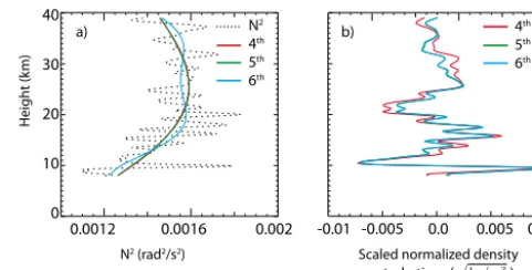
Figure 1. (a) Various (polynomial) fits of the local buoyancy

fre-quency squared (N2(z)), (b) corresponding scaled normalized den-sity perturbations.

By substituting the background density in the form defined by Eq. (2) and by omitting the notation of functional depen-dencies and introducing the notation da(z)_d_z =a0, we gain

N₀2= −g(−a−za0). (5)

Now it comes to the previously mentioned fact thatN₀2

generally evolves very weakly inside layers and with mod-erate jumps on boundaries. Hence, the frequency should be suitable for approximation by selected analytic functions. First, we must create a vertical profile of the perturbed lo-cal buoyancy frequency squared according to

N (z)2= − g

ρ(z)

d(ρ(z))

dz , (6)

which is illustrated in Fig. 1. Then, by fitting the perturbed frequency, we have the formula forN₀2and we can substitute it back to Eq. (5).

Further steps will be illustrated by the simple example of fitting the perturbed local buoyancy frequency squared by a fourth-order polynomial (see Fig. 1) in the form

A4z4+A3z3+A2z2+A1z+A0. (7)

After that we can substitute into Eq. (5) to get the first-order differential equation, which can be (after making a sub-stitutiony=a·z) directly solved to gain an expression for

a(z). Then going back to Eq. (2) we have:

ρ0(z)=

ˆ

ρ0exp −

A4z5

5 +

A3z4

4 +

A2z3

3 +

A1z2 2 +A0z

g −C

!

, (8)

whereAiandCare constants.

(4)

22 1

Figure 2. The dry temperature profile corresponding to the occultation event 2011-03-11 2

04:08:29 UTC. 3

4

5

50

40

30

20

10

0

210 220 230 240 250

H

ei

gh

t (

km

)

Dry temperature (K)

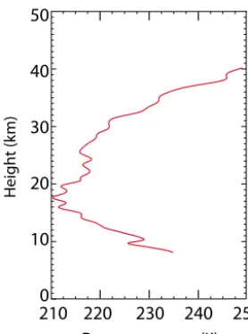
Figure 2. The dry temperature profile corresponding to the

occulta-tion event 11 March 2011, 04:08:29 UTC.

from the previously done fit of the perturbed local buoyancy frequency squared. For ρˆ0, the density value at the lower boundary can be chosen and the integration constant C as a correction toρ0can be assumed to be zero as a first guess. 2.2 Data description and methodology

The method of the density profile separation and identifica-tion of the IGWs is illustrated using data from the Constel-lation Observing System for Meteorology, Ionosphere and Climate (FORMOSAT3/COSMIC, Anthes et al., 2008). We have analysed a sample of 60 observational events spatiotem-porally nearest (prior as well as subsequent) to the 2011 Tohoku earthquake. From this sample, one representative RO profile was chosen from 11 March 2011, 04:08:29 UTC. This occultation event was used for illustration of the results where only a single profile is used. The dry temperature pro-file of this event is depicted in Fig. 2; note the inversion layer around 10 km altitude and the significantly perturbed tropopause. The whole sample of 60 events was averaged for the analysis and results described in Sect. 3.2.1.

Results are computed using only the “dry” profiles of density and temperature. The vertical extent of our analy-sis is 8–40 km and it includes the areas of two basic in-version algorithms for GPS RO – geometrical optics (GO) and radio holography (RH). At the COSMIC Data Analysis and Archive Center (CDAAC) RH (full spectrum inversion method in this case) is applied from ground to the upper tro-posphere and GO from there to the top of the profile. The vertical resolution is therefore variable across the height pro-file, but not less than 1.5 km (Melbourne, 2005). For details about the algorithms and discussion of their usage possibili-ties see e.g. Tsuda et al. (2011).

The used methodology is limited because the tropopause is included in the investigated vertical range too. In the tropopause region assumptions of the Wentzel, Kramers and Brillouin (WKB or ray tracing) theory, that background ve-locity and Brunt–Väisälä frequency vary slowly over a wave cycle (Fritts and Alexander, 2003), are violated. Using this theory we are treating the wave packets as particles mov-ing along rays (Sutherland, 2010) and usmov-ing the WKB ap-proximations we can relate the wave frequency to a wave’s spatial characteristics and background atmosphere properties through a dispersion relation as shown by Fritts and Alexan-der (2003). Polarization relations used for the determination of the IGWs’ parameters from temperature or density profile as proposed by Gubenko et al. (2011) are also a product of WKB approximations.

In the region where the ray theory is not valid, we can-not consider the amplitude envelope as slowly evolving and the relative phase, amplitude and spatial extent of the wave packet may change significantly as it evolves over time. Therefore the results are separated into the parts includ-ing the whole profile (8–40 km) and only the stratosphere (tropopause-40 km). In the whole vertical range, the typi-cal analysis method of vertitypi-cal wave number spectral den-sity (e.g. Steiner and Kirchengast, 2000; Tsuda and Hocke, 2002; Tsuda et al., 2011) would not make much sense as a consequence of the facts discussed above.

Relying only on the linear theory, we will present the re-sults of our method for background separation in the exten-sive region, using the continuous wavelet transform (CWT) and its skeleton as used by Chane-Ming et al. (2000). The wavelet transform was computed using the Morlet wavelet and algorithms proposed by Torrence and Compo (1998).

After the subtraction of the background density, the result-ing density perturbations are further normalized and scaled by the square root of the background density to conserve the kinetic energy as suggested by Hines (1960) and discussed by Sica and Russell (1999). Nevertheless, for the results in the stratospheric region alone, we use only the normalized density perturbations. Thus, we are able to compare directly the vertical wave-number spectra of the density and temper-ature perturbation and evaluate them with theoretical model spectra. This distinction, where needed, is emphasized in the following text.

3 Results

(5)

23 1

Figure 3. a) Various (polynomial) fits of the local buoyancy frequency squared (N2₍_z₎_{)in the} 2

stratosphere, b) corresponding normalized density perturbations. 3

4

5

-0.02 -0.01 0.0 0.01 0.02 2nd

3rd

4th

exp 40

30

20

10

0.0014 0.0016 0.0018 N2

2nd

3rd

4th

a) b)

40

30

20

10

H

ei

gh

t (

km

)

N2_(rad2_/s2₎ _{Normalized density perturbations}

10-4

10-5

10-6

10-7

10-8

10-9

0.1 1.0

PSD (k

m/c

ycle)

Wavenumber (cycle/km) 2nd

3rd

4th

exp temp. sat. spectrum

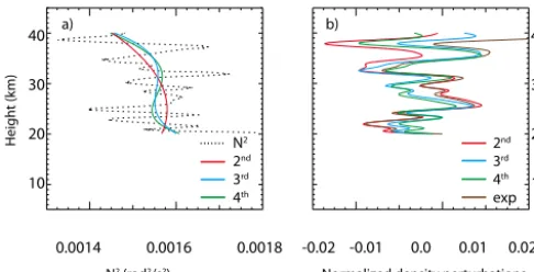
Figure 3. (a) Various (polynomial) fits of the local buoyancy

fre-quency squared (N2(z))in the stratosphere, (b) corresponding nor-malized density perturbations.

3.1 The background issue

In this subsection, the fits of the Brunt–Väisälä frequency squared are shown and discussed. Consequently, after appli-cation of our method, the resulting normalized and scaled density perturbation profiles are given. Additionally, the cor-responding forms of the temperature background are com-puted using the equation of state for dry air and the hy-drostatic balance. Conversely, background density profiles are calculated for various forms of background temperature functional dependence on altitude.

In the stratospheric region (in our case from tropopause up to 40 km), the results are derived using polynomial fits of

N2(z), starting with the second-order polynomial and ending with the fourth order. The second order is the lowest appro-priate one to capture the supposed nonlinear decay ofN₀2. On the other hand, higher order than the fourth-order polynomial can oscillate and even the fourth-order polynomial may gain a wave-like form in this narrow region. Considering the slow changes ofN₀2in the stratosphere and the limited vertical ex-tent of our region, we must be careful not to exaggerate the polynomial order, which could result in filtering of waves with vertical wavelengths in the interval of the IGWs’ likely appearance.

Chane-Ming et al. (2000) introduced a review of studies focused on the vertical wavelengths of dominant modes. In the area of our vertical range, the dominant vertical wave-lengths were smaller than 10 km. Considering the limited height range, Wang and Alexander (2010) suggested that the analysis be limited to vertical scales up to 15 km. Steiner and Kirchengast (2000) and most other relevant studies applied the analysis threshold of the IGWs around 10 km of the verti-cal wavelength. The lower boundary of analysed IGWs’ ver-tical wavelengths should be determined by the Nyquist fre-quency arising from the vertical resolution, but since the dis-cussion about the analysis range for studying IGWs is still open (Luna et al., 2013) we will examine a broad range of vertical scales.

Having theN₀2 profile in the form of a polynomial, the analytical form of the density background can be easily in-ferred from Eq. (8). An illustration of fits to the perturbed lo-cal buoyancy frequency squared and corresponding density perturbations are shown in Figs. 1 and 3. In Fig. 3 we added also the density perturbations resulting from the subtraction of the background in the form

ρ(z)=ρ0exp(−az), (9)

corresponding to an isothermal atmosphere. The other forms of the density background that we use are not so easily trans-ferable in the temperature space.

For example, even when we consider the density back-ground derived from linearN₀2profile

ρ(z)=ρ0exp −

A1z2 2 +A0z

g −C

!

. (10)

The background temperature profile can be derived as fol-lows. Assuming that the background state is the same for all quantities of state and that the background state is in hydro-static balance, we use the equation of state for dry air and the hydrostatic balance equation. After solving the differen-tial equations, the resulting background temperature profile has a quite complicated form:

T0(z)=exp _(A

1z+A0)2 2A1g

·K−

exph(A1z+A0)2 2A1g

i

g32 q

π 2Erf

A_√1z+A0

2A1g

√ A1R

, (11)

whereKis an integration constant,gis the gravitational ac-celeration andRis the gas constant.

If we analyse an inverse problem and try to find out which background density profile corresponds to frequently used temperature backgrounds, we discover that the polynomial fits of temperature are leading to an unphysical background in density space, generally looking like:

ρ0(z)≈

exp[−f (z)]

pol , (12)

wheref is non-specific function of zand pol denotes the original polynomial. Otherwise, if the temperature back-ground is written using goniometric functions, the resulting density profile behaves like an exponential, butf (z) has a very complicated form.

(6)

10-4

10-5

10-6

10-7

10-8

10-9

0.1 1.0

PSD (k

m/c

ycle)

Wavenumber (cycle/km)

2nd

3rd

4th

exp temp. sat. spectrum

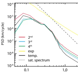
Figure 4. Vertical wave-number power spectral density for the

nor-malized density perturbations from different backgrounds and tem-perature normalized perturbations compared with the theoretical saturated spectra.

As we can see in Fig. 1a, the sixth-order polynomial gains a wavelike pattern with vertical wavelength of approximately 20 km, which is out of the interval of vertical scales normally considered to be gravity wave induced. Taking account of the temperature profile shown in Fig. 2, we can see in Fig. 1b that the tropopause (around 18 km) does not cause enhancement of the gravity wave activity unlike the inversion layer around 10 km altitude. The method is not able to assign correctly such meteorological phenomena with sharp changes of char-acteristics (as inversion layers) to the background, making them an artificial source of IGWs. In general, the perturba-tions are not biased and are centred around zero and due to the scaling, the decrease of the wave activity in the strato-sphere is clearly visible.

3.2 Comparison with temperature 3.2.1 In the stratosphere

In this section, we present a comparison between the normal-ized density perturbations resulting from the polynomial fits of N2(z)and the fit of the temperature profile with a cubic polynomial as used, for example, by Gubenko et al. (2008). We have computed the mean vertical wave-number power spectrum for the sample of 60 profiles. The vertical wave-number spectra of the normalized density and temperature perturbations are further compared with the theoretical shape of saturated spectra for density perturbations induced by the IGWs as derived by Senft and Gardner (1991).

The mean power spectral densities (PSDs) computed for various backgrounds and dry temperature for 60 profiles are depicted in Fig. 4. The presented range of vertical wave-lengths is from 20 km to 400 m. The lower frequency limit was chosen due to the vertical extent of the examined area and the higher frequency limit was chosen as 2 times the Nyquist frequency of the interpolation of data to the height

profile. According to Luna et al. (2013), the adequate choice of the wavelength cutoff for studying gravity waves through RO measurements is still open. For example, Wang and Alexander (2010) limited their analysis to vertical scales be-tween 4 and 15 km, Tsuda and Hocke (2002) applied no min-imum wavelength limit but Marquardt and Healy (2005) ar-gued that in the altitude region below 30 km only tempera-ture fluctuations with vertical wavelengths more than 2 km can be safely interpreted as originating from small-scale at-mospheric waves.

In Fig. 4 in the lower wave-number area, the influence of the background separation is dominant, with higher order fits giving lower powers. The fourth-order fit has the maximum shifted from roughly 12.5 to 7.5 km, unlike the other den-sity and temperature fits. That is a clear consequence of the higher possibility for this order fit to gain a wavelike form in this area (see Fig. 3a) and therefore the decrease of power in the long-wave part. For determination of whether such a long-wave mode is caused by IGW, more information (tem-perature, velocity, and so on) would be needed and then the polarization relations would have to be examined.

Between the vertical wavelengths of about 10 and 2.5 km, the spectra of density from all three fits and the temperature spectrum are similar and their slopes are in good agreement with the theoretically predicted slopes. An important fea-ture emerges at approximately 2.5 km, where the temperafea-ture fluctuation spectrum begins to decrease more rapidly than the density spectra regardless of the fit order. This should clearly be the consequence of the usage of hydrostatic balance in the temperature data retrieval, which excludes nonhydrostatic waves and, according to Steiner and Kirchengast (2000), acts to suppress wave amplitudes. The exponential fit (isothermal atmosphere) is failing to give correct orders of PSD values as well as to capture the feature of a saturated theoretical spec-trum.

3.2.2 Over the whole profile

Since we cannot rely on the theory (derived using WKB ap-proximations) in the full vertical extent, we have chosen the CWT (Torrence and Compo, 1998) method for analysis of the IGWs. Using CWT, we can study the behaviour of our method for the background separation in the tropopause re-gion and track the gravity wave activity behaviour depend-ing on altitude. Further, for the determination of dominant modes and for studying their development with height, we have applied a method of reducing CWT to its skeleton. We have used the same setting for drawing the spectral lines as Chane-Ming et al. (2000).

(7)

P. Šácha et al.: Analysis of internal gravity waves with GPS RO density profiles 4129

24 perturbations from different backgrounds and temperature normalized perturbations compared 2

with the theoretical saturated spectra. 3

4

5

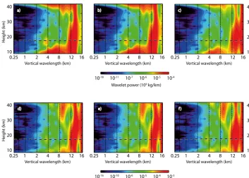
Figure 5. Wavelet power spectra of various perturbations resulting from different background 6

states: Scaled normalized density perturbations resulting from the 6th (a), 5th (b) and 4th (c) 7

order polynomial fits; Normalized density perturbations resulting from the 6th (d) and 5th (e) 8

order polynomial fits; Normalized dry temperature perturbations resulting from the 6th (f) 9

order polynomial fit. 10

10-18₁₀-11₁₀-7₁₀-6₁₀-5₁₀-4

40

30

20

10

40

30

20

10

H

ei

gh

t (

km

)

H

ei

gh

t (

km

)

0.25 1 2 4 8 12 16

Vertical wavelength (km)

Wavelet power (109_kg/km) 0.25 1 2 4 8 12 16

0.25 1 2 4 8 12 16

a) b) c)

10-16₁₀-10₁₀-6₁₀-5₁₀-4₁₀-3

40

30

20

10

40

30

20

10

H

ei

gh

t (

km

)

H

ei

gh

t (

km

)

0.25 1 2 4 8 12 16

Wavelet power (km2₎ 0.25 1 2 4 8 12 16

0.25 1 2 4 8 12 16

d) e) f)

Figure 5. Wavelet power spectra of various perturbations resulting from different background states: scaled normalized density perturbations

resulting from the (a) sixth-, (b) fifth- and (c) fourth-order polynomial fits; normalized density perturbations resulting from the (d) sixth- and

(e) fifth-order polynomial fits; normalized dry temperature perturbations resulting from the (f) sixth-order polynomial fit.

separation of the background in the form of a sixth-order polynomial are shown in Fig. 5f.

The differences between CWTs of different fits as well as between the scaled and unscaled perturbations point to char-acteristic features. The differences between different fits are, as expected, most pronounced in the region of the longer ver-tical wavelengths. This is even more evident when compar-ing the skeletons of CWT in Fig. 6. In general, the differ-ence between the scaled and unscaled perturbations is mainly connected with the theoretically predicted decrease of wave activity in the stratosphere and the shift of wave activity to longer wavelengths with height due to gradual filtering of small-wavelength IGWs above the troposphere (Fritts and Alexander, 2003). That is captured better by the CWT of the scaled perturbations. Nevertheless, there are also unexpected differences between the scaled and unscaled CWTs in the region of wavelengths around 16 km, where the amplitude is around one order higher and constant with height for the scaled case. The temperature CWT behaves similarly to that of the unscaled density perturbations.

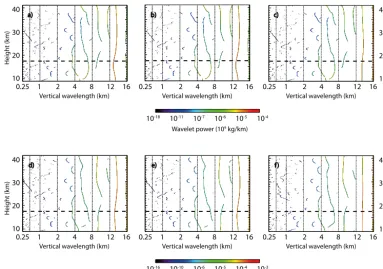
Spectral lines of the CWTs’ maxima are plotted in Fig. 6a– f in the same order as in Fig. 5a–f. From comparison of Fig. 6a–c, we can infer that the dominant mode with the wavelength around 16 km is probably caused by low-quality separation of background. We can argue this because in the cases of the temperature perturbations (Figs. 5f and 6f) and fourth-orderN2(z)fit (Figs. 5c and 6c) where this mode is

the strongest, it has height-constant wavelength regardless of the variable local stability.

Other dominant modes occurring across the different fits and across the whole profile have scales around 13 km and approximately from 5 to 7 km. The skeletons should be com-pared with theN₀2profiles in Fig. 1a because according to, for example, Chane-Ming et al. (2000) the change of the ver-tical wavelength of individual modes with height should be inversely proportional to the local stability.

In our case, in the upper stratosphere, the decreasing wave-length of modes with height suggests the role of nonlinear wave processes acting to limit the amplitude which is re-flected by the cessation of the wavelength growth. On the other hand, in the upper troposphere/lower stratosphere re-gion where, in our case, the stability is growing, we can find increasing wavelength with height, which is evident for ex-ample for the mode with scale of 5–7 km in Fig. 6a. This sug-gests the possible enhancement of this mode’s amplitude by means of wave–wave interactions or possible amplification resulting from some instabilities in the tropopause region.

4 Summary and conclusions

(8)

25 1

Figure 6. Wavelet power spectra skeletons of various perturbations resulting from different 2

background states: Scaled normalized density perturbations resulting from the 6th (a), 5th (b) 3

and 4th (c) order polynomial fits; Normalized density perturbations resulting from the 6th (d) 4

and 5th (e) order polynomial fits; Normalized dry temperature perturbations resulting from 5

the 6th (f) order polynomial fit. 6

10-18₁₀-11₁₀-7₁₀-6₁₀-5₁₀-4 40

30

20

10

40

30

20

10

H

ei

gh

t (

km

)

H

ei

gh

t (

km

)

0.25 1 2 4 8 12 16

Wavelet power (109_kg/km)

0.25 1 2 4 8 12 16

a) b) c)

10-16₁₀-10₁₀-6₁₀-5₁₀-4₁₀-3 40

30

20

10

40

30

20

10

H

ei

gh

t (

km

)

H

ei

gh

t (

km

)

0.25 1 2 4 8 12 16

Wavelet power (km2₎

0.25 1 2 4 8 12 16

d) e) f)

Figure 6. Wavelet power spectra skeletons of various perturbations resulting from different background states: scaled normalized density

perturbations resulting from the sixth- (a), fifth- (b) and (c) fourth-order polynomial fits; normalized density perturbations resulting from the sixth- (d) and (e) fifth-order polynomial fits; normalized dry temperature perturbations resulting from the (f) sixth-order polynomial fit.

and comparison of resulting IGWs’ analyses from density profiles with those from temperature profiles was discussed with regard to theory.

In the process of deriving our method in Sect. 2.1, we de-scribed the quantities defined by Eqs. (3), (4) and (5) as the Brunt–Väisälä or buoyancy frequency. Although this helps to introduce and to understand the separation method, it might be also seen as phenomenologically inconsistent. Such a de-scription would be correct for a fluid where the density is in-dependent of pressure and the density of a fluid particle could be considered unchanged when it was displaced vertically (Sutherland, 2010). In our case this is not true. Therefore, a different naming convention should be used for these quan-tities in future work. For example, using the density scale height (Hρ)definition (e.g. Sutherland, 2010), Eq. (3) can be written as

g Hρ

. (13)

Nevertheless, the naming convention has no influence on the results.

In Sect. 3.1, the problems of the background choice are discussed, correspondence between analytical forms of den-sity and temperature background profiles is examined and the non-physicality of polynomial temperature fit is shown by solving a related differential equation.

A very important result is shown in Sect. 3.2.1. In the high wave-number region from approximately 0.4 cycle km−1 (2.5 km vertical wavelength), the power spectrum of the nor-malized fluctuations derived from dry temperature GPS RO data has lower values than for normalized density fluctua-tions regardless of the background type. Steiner and Kirchen-gast (2000) argued that the likely causes of a tendency of increasing underestimation of spectral power towards higher wave numbers are the GO technique, the local spherical sym-metry assumption and the hydrostatic equilibrium assump-tion. The last of these is confirmed by our results.

(9)

may be already filtered by the local spherical symmetry as-sumption.

In Sect. 3.2.2, the results of CWT and its skeleton do not reveal noticeable differences between the dry temperature and density based IGW analyses. Rather the differences be-tween the scaled and unscaled cases are more important and the role of subjective background choice has visible influ-ence on the longer modes. We do not discuss the propagation or sourcing of waves, which could be tempting especially in the case of modes emerging or ending suddenly in the pro-file. The GPS RO measurement is a “snapshot” of the real atmosphere and no information from the cotangent space is included. Hence, using just a simple profile, we cannot say if or in which direction the mode propagates. Special care must be taken also when interpreting the results of the CWT skele-ton because the vertical behaviour of modes could be also a consequence of fluctuation retrieval rather than of physical processes. That can be seen in Fig. 6 from comparison of the dominant modes between 4 and 8 km vertical wavelength in the upper stratosphere.

In summary, the analysis of IGWs with the GPS RO den-sity profiles bears advantages over the analysis from dry tem-perature profile. Primarily, unlike the temtem-perature, the den-sity background has a familiar form and the consequent anal-ysis is not restricted to hydrostatic waves.

Acknowledgements. The study was supported by the Charles

University in Prague, project GA UK No. 108313, by the Aktion program, by grant no. SVV-2014-26096, and by the Austrian Science Fund (FWF; BENCHCLIM project P22293-N21. UCAR/CDAAC (Boulder, CO, USA) is acknowledged for the provision of RO data. Finally we thank Andrea K. Steiner (WEGC, University of Graz) for fruitful discussions.

Edited by: J. Y. Liu

References

Alexander, P., de la Torre, A., Llamedo, P., Hierro, R., Schmidt, T., Haser, A., and Wickert, J.: A method to improve the determina-tion of wave perturbadetermina-tions close to the tropopause by using a dig-ital filter, Atmos. Meas. Tech., 4, 1777–1784, doi:10.5194/amt-4-1777-2011, 2011.

Anthes, R. A., Bernhardt, P. A., Chen, Y., Cucurull, L., Dymond, K. F., Ector, D., and Thompson, D. C.: THE COSMIC/FORMOSAT-3 MISSION Early Results, B. Am. Me-teorol. Soc., 89, 313–333, doi:10.1175/BAMS-89-3-313, 2008. Chane-Ming, F., Molinaro, F., Leveau, J., Keckhut, P., and

Hauchecorne, A.: Analysis of gravity waves in the tropical mid-dle atmosphere over La Reunion Island (21◦S, 55◦E) with lidar using wavelet techniques, Ann. Geophys., 18, 485–498, doi:10.1007/s00585-000-0485-0, 2000.

Chiu, Y. T. and Ching, B. K.: The response of atmospheric and lower ionospheric layer structures to gravity waves, Geophys. Res. Lett., 5, 539–542, 1978.

Cushman-Roisin, B.: Introduction to Geophysical Fluid Dynamics, Prentice Hall, Englewood Cliff , New Jersey 07632, 1994. Ern, M., Preusse, P., Gille, J. C., Hepplewhite, C. L., Mlynczak, M.

G., Russell, J. M., and Riese, M.: Implications for atmospheric dynamics derived from global observations of gravity wave mo-mentum flux in stratosphere and mesosphere, J. Geophys. Res.-Atmos., 116, D19107, doi:10.1029/2011JD015821, 2011. Foelsche, U., Borsche, M., Steiner, A. K., Gobiet, A., Pirscher, B.,

Kirchengast, G., and Schmidt, T.: Observing upper troposphere– lower stratosphere climate with radio occultation data from the CHAMP satellite, Clim. Dynam., 31, 49–65, 2008.

Fritts, D. C. and Alexander, M. J.: Gravity wave dynamics and eff ects in the middle atmosphere, Rev. Geophys., 41, 1003, doi:10.1029/2001RG000106, 2003.

Garcia, R. R. and Randel, W. J.: Acceleration of the Brewer-Dobson circulation due to increases in greenhouse gases, J. Atmos. Sci., 65, 2731–2739, 2008.

Gardner, C. S. and Shelton, J. D.: Density response of neutral atmo-spheric layers to gravity wave perturbations, J. Geophys. Res.-Space, 90, 1745–1754, 1985.

Gardner, C. S., Senft, D. C., Beatty, T. J., Bills, R. E., and Hostetler, C. A.: Rayleigh and sodium lidar techniques for measuring mid-dle atmosphere density, temperature and wind perturbations and their spectra, in: World Ionosphere/Thermosphere Study, Volume 2, edited by: Liu, C. H., Chapter 6, University of Illinois, 1406 W. Green St., Urbana, Illinois 61801. 148–187, December 1989. Gubenko, V. N., Pavelyev, A. G., and Andreev, V. E.: Determination of the intrinsic frequency and other wave parameters from a sin-gle vertical temperature or density profile measurement, J. Geo-phys. Res.-Atmos., 113, D08109, doi:10.1029/2007JD008920, 2008.

Gubenko, V. N., Pavelyev, A. G., Salimzyanov, R. R., and Pave-lyev, A. A.: Reconstruction of internal gravity wave 5 parameters from radio occultation retrievals of vertical temperature profiles in the Earth’s atmosphere, Atmos. Meas. Tech., 4, 2153–2162, doi:10.5194/amt-4-2153-2011, 2011.

Gubenko, V. N., Pavelyev, A. G., Salimzyanov, R. R., and An-dreev, V. E.: A method for determination of internal gravity wave parameters from a vertical temperature or density profile mea-surement in the Earth’s atmosphere, Cosmic Res., 50, 21–31, doi:10.1134/S0010952512010029, 2012.

Hines, C. O.: Internal atmospheric gravity waves at ionospheric heights, Can. J. Phys., 38, 1441–1481, 1960.

Liou, Y. A., Pavelyev, A. G., Huang, C. Y., Igarashi, K., Hocke, K., and Yan, S. K.: Analytic method for observation of the grav-ity waves using radio occultation data, Geophys. Res. Lett., 30, 2021, doi:10.1029/2003GL017818, 2003.

Liou, Y. A., Pavelyev, A. G., and Wickert, J.: Observation of the gravity waves from GPS/MET radio occultation data, J. Atmos. Sol.-Terr. Phys., 67, 219–228, 2005.

Luna, D., Alexander, P., and de la Torre, A.: Evaluation of uncer-tainty in gravity wave potential energy calculations through GPS radio occultation measurements, Adv. Space Res., 52, 879–882, doi:10.1016/j.asr.2013.05.015, 2013.

Markwardt, C. B.: Non-linear least squares fitting in IDL with MP-FIT, arXiv preprint arXiv:0902.2850, 2009.

(10)

obtained from GPS occultation data, J. Meteorol. Soc. Jpn., 83, 417–428, 2005.

Marshall, A. G. and Scaife, A. A.: Impact of the QBO on sur-face winter climate, J. Geophys. Res.-Atmos., 114, D18110, doi:10.1029/2009JD011737, 2009.

Melbourne, W. G.: Radio occultations using Earth satellites: a wave theory treatment, Vol. 5, Wiley-Blackwell, ISBN 0-471-71222-1, 2005.

Pavelyev, A. G., Wickert, J., Liou, Y. A., Pavelyev, A. A., and Ja-cobi, J.: Analysis of atmospheric and ionospheric wave structures using the CHAMP and GPS/MET radio occultation database, in: Atmosphere and Climate Studies by Occultation Methods, edited by: Foelsche, U., Kirchengast, G., and Steiner, A., Springer Ver-lag, Springer Berlin Heidelberg, 225–242, doi:10.1007/3-540-34121-8_19, 2006.

Pavelyev, A. G., Liou, Y. A., Wickert, J., Gubenko, V. N., Pave-lyev, A. A., and Matyugov, S. S.: New Applications and Ad-vances of the GPS Radio Occultation Technology as Recov-ered by Analysis of the FORMOSAT-3/COSMIC and CHAMP Data-Base, in: New Horizons in Occultation Research: Studies in Atmosphere and Climate, edited by: Steiner, A., Pirscher, B., Foelsche, U., Kirchengast, G., Springer, Berlin Heidelberg, 165– 178, doi:10.1007/978-3-642-00321-9, 2009.

Preusse, P., Eckermann, S. D., and Ern, M.: Transparency of the at-mosphere to short horizontal wavelength gravity waves, J. Geo-phys. Res.-Atmos., 113, D24104, doi:10.1029/2007JD009682, 2008.

Schmidt, T., Wickert, J., De la Torre, A., Alexander, P., Faber, A., Llamedo, P., and Heise, S.: The effect of different background separation methods on gravity wave parameters in the upper tro-posphere and lower stratosphere region derived from GPS radio occultation data, in: 39th COSPAR Scientific Assembly, Vol. 39, July, 1721 pp., 2012.

Schreiner,W., Rocken, C., Sokolovskiy, S., Syndergaard, S., and Hunt, D.: Estimates of the precision of GPS radio occultations from the COSMIC/FORMOSAT-3 mission, Geophys. Res. Lett., 34, L04808, doi:10.1029/2006GL027557, 2007.

Senft, D. C. and Gardner, C. S.: Seasonal variability of gravity wave activity and spectra in the mesopause region at Urbana, J. Geo-phys. Res.-Atmos., 96, 17229–17264, 1991.

Sica, R. and Russell, A.: Measurements of the eff ects of gravity waves in the middle atmosphere using parametric models of den-sity fluctuations. Part I: vertical wavenumber and temporal, J. At-mos. Sci., 56, 1308–1329, 1999.

Steiner, A. K. and Kirchengast, G.: Gravity Wave Spectra from GPS/MET Occultation Observations, J. Atmos. Ocean. Tech., 17, 495–503, 2000.

Sutherland, B.: Internal Gravity Waves, Cambridge University Press, ISBN:9780521839150, 2010.

Tsuda, T. and Hocke, K.: Vertical wave number spectrum of temper-ature fluctuations in the stratosphere using GPS occultation data, J. Meteorol. Soc. Jpn., 80, 925–938, doi:10.2151/jmsj.80.925, 2002.

Tsuda, T., Nishida, M., Rocken, C., and Ware, R. H.: A global mor-phology of gravity wave activity in the stratosphere revealed by the GPS occultation data (GPS/MET), J. Geophys. Res.-Atmos., 105, 7257–7273, 2000.

Tsuda, T., Lin, X., Hayashi, H., and Noersomadi: Analysis of ver-tical wave number spectrum of atmospheric gravity waves in the stratosphere using COSMIC GPS radio occultation data, At-mos. Meas. Tech., 4, 1627–1636, doi:10.5194/amt-4-1627-2011, 2011.

Torrence, C. and Compo, G. P.: A practical guide to wavelet analy-sis, B. Am. Meteorol. Soc., 79, 61–78, 1998.

Vincent, R. A., Allen, S. J., and Eckermann, S. D.: Gravity-wave parameters in the lower stratosphere, in: Gravity Wave Processes, Springer, Berlin Heidelberg, 7–25, 1997.

Wang, L. and Alexander, M. J.: Global estimates of gravity wave parameters from GPS radio occultation temperature data, J. Geo-phys. Res.-Atmos., 115, D21122, doi:10.1029/2010JD013860, 2010.

Wickert J., Schmidt T., Michalak G., Heise S., Arras C., Beyerle G., Falck C., König R., Pingel D., and Rothacher M.:GPS ra-dio occultation with CHAMP, GRACE-A, SAC-C, TerraSAR-X, and FORMOSAT-3/COSMIC: brief review of results from GFZ, in: New horizons in occultation research, edited by: Steiner, A., Pirscher, B., Foelsche, U., Kirchengast, G., Springer, Berlin Hei-delberg, 3–15, doi:10.1007/978-3-642-00321-9, 2009.

Wilson, R., Chanin, M. L., and Hauchecorne, A.: Gravity waves in the middle atmosphere observed by Rayleigh lidars. Part 2: Climatology, J. Geophys. Res., 96, 5169–5183, 1991.