www.drink-water-eng-sci.net/9/19/2016/ doi:10.5194/dwes-9-19-2016
© Author(s) 2016. CC Attribution 3.0 License.
Estimating fast and slow reacting components in surface
water and groundwater using a two-reactant model
Priyanka Jamwal1, M. N. Naveen1,2, and Yusuf Javeed2
1Centre for Environment and Development, Ashoka Trust for Research in Ecology and the Environment
(ATREE), Jakkur 560064, India
2Department of Civil engineering, The National Institute of Engineering, Mysuru, Karnataka 570008, India Correspondence to: Priyanka Jamwal ([email protected])
Received: 11 September 2015 – Published in Drink. Water Eng. Sci. Discuss.: 22 October 2015 Revised: 21 April 2016 – Accepted: 25 April 2016 – Published: 18 May 2016
Abstract. Maintaining residual chlorine levels in a water distribution network is a challenging task, especially
in the context of developing countries where water is usually supplied intermittently. To model chlorine decay in water distribution networks, it is very important to understand chlorine kinetics in bulk water. Recent studies have suggested that chlorine decay rate depends on initial chlorine levels and the type of organic and inorganic matter present in water, indicating that a first-order decay model is unable to accurately predict chlorine decay in bulk water. In this study, we employed the two-reactant (2R) model to estimate the fast and slow reacting components in surface water and groundwater. We carried out a bench-scale test for surface water and groundwater at initial chlorine levels of 1, 2, and 5 mg L−1. We used decay data sets to estimate optimal parameter values for both surface water and groundwater. After calibration, the 2R model was validated with two decay data sets with varying initial chlorine concentrations (ICCs). This study arrived at three important findings. (a) We found that the ratio of slow to fast reacting components in groundwater was 30 times greater than that of the surface water. This observation supports the existing literature which indicates the presence of high levels of slow reacting fractions (manganese and aromatic hydrocarbons) in groundwater. (b) Both for surface water and groundwater, we obtained good model prediction, explaining 97 % of the variance in data for all cases. The mean square error obtained for the decay data sets was close to the instrument error, indicating the feasibility of the 2R model for chlorine prediction in both types of water. (c) In the case of deep groundwater, for high ICC levels (> 2 mg L−1),
the first-order model can accurately predict chlorine decay in bulk water.
1 Introduction
The presence of 0.2 mg L−1 of residual chlorine in drink-ing water is known to reduce public health risks significantly (Arnold and Colford, 2007; Pattanayak et al., 2005). One of the key tasks of water managers worldwide, especially in de-veloping nations, is to maintain residual chlorine levels of drinking water in distribution systems. This requires a higher concentration at entry point in order to ensure that a minimal residual chlorine concentration of 0.2 mg L−1 is retained at any point of time before reaching the end consumers.
To maintain 0.2 mg L−1 of residual chlorine in water, sodium hypochlorite or liquid chlorine is added to the treated
A first-order decay process is generally employed to sim-ulate chlorine decay within the distribution network (Hua et al., 1999; Rossman et al., 1994; Vasconcelos et al., 1997). The model assumes that chlorine decay rate is a function of chlorine levels within the bulk water. However, recent studies have shown that in addition to chlorine levels, other factors like the type of organic/inorganic matter, temperature, and pipe material also affect chlorine decay rates in the distribu-tion system (Al-Jasser, 2007; Mutoti et al., 2007; Hallam et al., 2002).
The total chlorine decay within the water distribution net-work is caused by chlorine reaction (a) in bulk water and (b) with the biofilm attached to the pipe surface, also termed wall decay (Al-Jasser, 2007; Hallam et al., 2002; Powell et al., 2000). For prediction of chlorine decay over time, models require accurate estimation of chlorine reaction in bulk water and with the biofilm on the pipe wall surface. Pilot loop set-ups/simulators are employed to estimate the contribution of wall reactions to chlorine decay (Frias et al., 2001; Lehtola et al., 2006; Rossman et al., 1994, 2006). This is achieved by subtracting the bulk reaction rate from the total chlorine de-cay rate in the pipe loop. Various authors have argued about the need to accurately model bulk decay before making an attempt to estimate the contribution of wall decay (Fisher et al., 2011).
Chlorine decay kinetics depends on the type and amount of dissolved organic matter (DOM) and inorganic matter present in bulk water. DOM is derived primarily from decay-ing organisms such as plants or algae, and is often classified into humic and non-humic substances such as proteins, car-bohydrates, and lipids. Generally speaking, DOM from ma-rine and aquatic sources is more enriched in aliphatic struc-tures, while DOM from terrestrial/higher plant sources is rich in aromatic compounds (Chen et al., 2010). The inorganic compounds in surface water are derived from the dissolution of minerals present in the bedrock as water flows, whereas groundwater dissolves minerals as it percolates through the vadose zone as well as during its stay in the saturated zone. Therefore, in comparison to surface water, groundwater con-tains high levels of inorganic substances such as nitrates, manganese, arsenic, and iron.
Several studies have shown that in homogeneous systems, chlorine exhibits faster reaction rates with ammonia, sulfates, nitrates, nitrites, arsenic, and iron as compared to manganese (Mn (II)) (Deborde and Von Gunten, 2008). Therefore, given different characteristics of the components (organic and inor-ganic) present in surface water and groundwater, the precur-sors to chlorine reactions can be divided into fast and slow reacting fractions (Gallard and von Gunten, 2002). Table 1 presents the list of possible fast and slow reacting compo-nents in different types of water.
The two-reactant model (2R model) is a simplified second-order decay model which uses notional fast and slow reacting agents involved in second-order reactions with chlorine over long travel periods within the distribution network (Fisher et
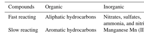
Table 1.Fast and slow reacting components present in different types of water.
Compounds Organic Inorganic
Fast reacting Aliphatic hydrocarbons Nitrates, sulfates, ammonia, and nitrites Slow reacting Aromatic hydrocarbons Manganese Mn (II)
al., 2011). The second-order reaction rates and the resulting 2R model are given by the following equations:
dCf
dt = −Kf·Cf·Ccl, (1)
dCs
dt = −Ks·Cs·Ccl, (2)
dCcl
dt =
dCf
dt +
dCs
dt , (3)
where Ccl is the concentration of residual chlorine levels
(mg L−1),CfandCsare the concentrations of fast and slow
reducing agents (mg L−1), and Kf and Ks are the fast and
slow reaction rate coefficients (L mg−1h−1).
The initial concentration of fast and slow reactants (Cos
andCof) and their respective decay coefficients (KsandKf)
can be estimated using the AQUASIM software (Fisher et al., 2011).
So far, first- and second-order chlorine decay models have been calibrated and tested for different types of test wa-ter under varying conditions such as temperature, type of treatment, and re-chlorination (Fisher et al., 2012; Mutoti et al., 2007; Rossman, 2006). All prior studies have esti-mated the chlorine decay parameters for water from differ-ent sources (variable water quality). The results obtained are specific and suitable for predicting chlorine decay in water supply networks of the source water for which the studies were conducted. This study aims to estimate the chlorine de-cay parameters using the 2R model relevant to local condi-tions found in southern India, where hard rock aquifers are abundant, and compare them with surface water parameters. We employed the 2R model to estimate optimal parameters for prediction of residual chlorine in both surface water and groundwater. The model was calibrated separately for test water with initial chlorine levels ranging from 1 to 5 mg L−1.
To establish the suitability of the 2R model, we also validated it against two chlorine decay data sets.
2 Methodology
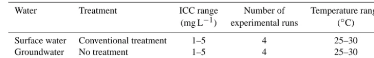
Table 2.Characteristics of the data set.
Water Treatment ICC range Number of Temperature range
(mg L−1) experimental runs (◦C)
Surface water Conventional treatment 1–5 4 25–30
Groundwater No treatment 1–5 4 25–30
2.1 Chlorine decay data sets
Chlorine decay tests and data for calibration and validation of the 2R model were obtained by conducting bench-scale residual chlorine decay tests at the ATREE water and soil laboratory.
Groundwater and surface water samples were obtained from the respective sources and water quality characteris-tics were determined as presented in Table 3. The test water was stored in amber glass bottles, while sodium hypochlo-rite was added to attain the desired initial chlorine concen-trations (ICCs). The bench-scale tests for both types of water were run at ICC-1, 2, 4.5, and 5 mg L−1. The amber glass
bottles were kept in an incubator set at ambient temperature (25 to 30◦C). During the day, hourly samples were drawn from the bottles and free chlorine levels were measured for 72 h. Free chlorine in the test water was measured using a Merck Spectroquant® Picco colorimeter. The free chlorine measurement range of the instrument is 0.05 to 6.00 mg L−1 (APHA, 2005). The decay test results obtained were within the measurement range of the instrument.
2.2 Model parameter estimation
The AQUASIM software was used to estimate optimal pa-rameter values for the 2R model to obtain the best fit for the three decay data sets (ICC-1, 2, and 5 mg L−1; bench-scale laboratory experiments). Optimal parameters are the values that allow the model to predict chlorine decay in each type of water as accurately as possible. As explained by Fisher et al. (2012), the AQUASIM software calculates the sum of squared differences between each experimental data point and the corresponding model prediction, assuming an initial set of parameter values. This sum is derived by the variance of the data to form a chi square (χ2). Using the simplex tech-nique it then systematically varies the parameter values to search for a set that produces the best fit (minimizesχ2). The coefficient of determination (R2) was also obtained which in-dicates the total variance in the data set explained by the 2R model regardless of the distance between the decay curves. To measure the 2R model accuracy for chlorine prediction, we also estimated the root mean square error (RMSE) for the data sets.
We calibrated the 2R model using chlorine decay data sets for initial chlorine levels of 1, 2, and 5 mg L−1. The opti-mal parameters for groundwater and surface water were de-termined separately. After calibration, the 2R model was
val-idated using two data sets, i.e. of ICC-2 mg L−1 (a subset of the calibration data set) and ICC-4.5 mg L−1(independent chlorine decay data set).
3 Results
3.1 Chlorine decay and water quality
The results of bench-scale chlorine decay tests are presented in Fig. 1. The graph presents the fraction of chlorine remain-ing in test water at different ICCs. The data present two inter-esting findings: (i) the decay rate decreases with an increase in initial chlorine levels and (ii) the chlorine decay rate in surface water is greater than that of groundwater. The above results are in conjugation with the other studies that suggest that the first-order decay model is unable to predict chlorine decay in bulk water, and the chlorine decay rate depends on the ICC and level of organic/inorganic matter present in the test water (Fisher et al., 2011; Hua et al., 1999; Rossman, 2006).
As shown in Table 2, the ambient temperature during this study fluctuated between 25 and 30◦C. The
tempera-ture alone could not explain the variation in the first-order decay constant at different ICCs. Therefore we employed the 2R model to predict the chlorine decay in bulk water. As per the literature review, none of the earlier studies have used the 2R model to estimate fast and slow reacting compo-nents of groundwater from deep hard rock aquifers. Fisher et al. (2011) estimated decay parameters for shallow and deep groundwater from the Wanneroo aquifer (Fisher et al., 2015; Warton et al., 2006), which could not be applied as-is to predict chlorine decay in deep groundwater from hard rock aquifers. The decay parameter, estimated by the 2R model, depends on the quality of the source water. Therefore in this study, an attempt has been made to estimate decay parame-ters specific to the local water sources and conditions.
In the next section, we employ the 2R model to estimate fast and slow reacting components in test waters. In addition, we will also test the feasibility of the 2R model in predicting chlorine decay in test waters.
3.2 2R model calibration and validation
Table 3.Water quality parameters of test water.
Parameter Surface water Standard deviation Groundwater Standard deviation
(n=3) (n=3)
pH 7.19 0.47 6.75 0.01
Conductivity (muS cm−1) 434 30 1150 17
Nitrates (mg L−1) 3 1 177 20
Hardness (mg L−1) 180 56 352 8
Alkalinity (mg L−1) 196 4 165 3
Figure 1. Fraction of chlorine remaining in surface water and groundwater at different initial chlorine levels.
The 2R model predicted optimal values for four param-eters simultaneously by minimizing the chi-squared (χ2) value. Minimization of χ2 was readily achieved using the optimization technique available within the AQUASIM pa-rameter estimation procedure. The optimal values with the associatedχ2value are presented in Table 4.
Figure 2 presents the decay curves obtained from the sim-ulation using optimized parameter values for the calibration data sets. We observed good agreement between chlorine residual data and the model estimates for all ICCs, both for surface water and groundwater.
Theχ2values obtained for surface water and groundwa-ter were 0.18 and 0.48, respectively. The R2 values were greater than 0.98 for surface water and 0.99 for groundwa-ter, indicating that only 2 and 1 % variance in the
calibra-Figure 2.Chlorine decay in surface water (a) and groundwater (b): markers – measured chlorine values; curves – values simulated by 2R models.
Table 4.Comparison of optimal parameter values obtained for different test waters.
Source Treatment ICC range Cof Cos Kf Ks Cos/Cof χ2 R2 type (mg L−1) (mg L−1) (mg L−1) (L mg−1h−1) (L mg−1h−1)
Surface water1 Conventional treatment 1–5 0.51 2.88 2.55 0.0069 6 0.18 0.978 Groundwater1 No treatment 1–5 0.003 0.67 8.07 0.013 223 0.48 0.998 Surface water2 Conventional treatment 1–4 0.808 3.88 0.261 0.0102 5 0.18 0.992 Surface water2 No treatment 1–4 0.761 2.69 0.199 0.0066 4 0.97 0.987 Surface water2 Not known 1–4 0.917 1.98 6.18 0.085 2 0.844 0.987
1Bench-scale test (our study).2Bench-scale test (Fisher et al., 2012).
In groundwater, the ratio of slow to fast reacting compo-nents was 30 times greater than that of the surface water. This suggests that, as groundwater travels through the vadose zone, most of the fast reacting organic matter is consumed by microorganisms, leaving behind the non-biodegradable or-ganic/inorganic matter (slow reacting component) (He et al., 2006; McCarty et al., 1981). The slow reacting components are difficult to oxidize; therefore, over time, high levels of residual chlorine were observed in groundwater. It also sug-gests that in the absence of fast reacting components, first-order decay models could accurately predict chlorine decay in groundwater at ICCs greater than 2 mg L−1.
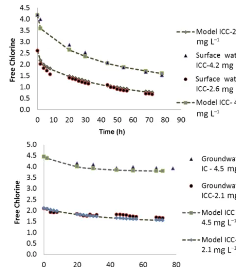
3.3 Validation of the 2R model
The 2R model was fitted for experimental data sets – (a) sur-face water (ICC-2.6 and 4.2 mg L−1) and (b) groundwater (ICC-2 and 4.5 mg L−1), as shown in Fig. 3.
First we calibrated the 2R model with decay data sets, commencing with the highest and lowest ICCs, as the extrap-olation outside the calibration range is less reliable. Then we validated the model by using two chlorine decay data sets, i.e. one from the calibration data set (ICC-2 mg L−1) and one from the other data set that has not been used for the model calibration (ICC-4 mg L−1).
The R2 value obtained for both the data sets of surface water was greater than 0.98, indicating that only 2 % of the variance remains unexplained by the 2R model. This sug-gests the suitability of the 2R model for chlorine prediction in surface water. In the case of groundwater,R2values of 0.89 and 0.94 were obtained for decay tests at 2 and ICC-4.5 mg L−1, respectively. The reason for the lowerR2values for the validated data for groundwater is thatR2is a measure of fit involving the error relative to the variance in the data. The groundwater data have lower variance than surface water data and at lower ICC groundwater data have lower variance than the higher ICC data. Therefore, even with the same level of error in all data, the groundwater chlorine decay data sets showed lowR2values as compared to the surface water chlo-rine decay data sets.
To check the prediction accuracy of the 2R model, we estimated the mean square error for both surface water and groundwater data sets. The values obtained were±0.07 and
Figure 3.Validation of the 2R model for surface water and ground-water at different ICCs.
±0.05 mg L−1 for surface water and groundwater, respec-tively, which is close to the instrument measurement error (±0.05 mg L−1). This indicates that the parameter estimates
obtained could accurately predict chlorine decay in surface water and groundwater.
4 Conclusions
For both types of water, the observed chlorine residual val-ues in bulk water closely matched the 2R model predicted values (ICC-1 to 5 mg L−1). The 2R model calibration and
validation range was well within the chlorine residual range encountered in water distribution networks (0–6 mg L−1). Therefore, we can conclude with a reasonable degree of con-fidence that these invariant sets of model parameters obtained for surface water and groundwater if used in conjunction with the EPANET-MSX (Multi-Species extension) model will sig-nificantly assist public utilities in dealing with water quality issues in water distribution networks.
This study is also important in the context of urban ar-eas in developing countries where 50 % of the water demand (Deccan plateau region – southern India) is met by ground-water pumping (Grönwall et al., 2010). The groundground-water is pumped to overhead tanks, chlorinated, and supplied through a piped water connection. As stated above, the results of this study in conjunction with a sufficiently accurate prediction of wall decay will enable water management agencies to de-termine the ICC levels that allow residual targets at system extremities to be met.
Acknowledgements. Financial support for this research came from the Department of Science and Technology, Government of India grant number SR/FTP/ETA-91/2010 titled “Water Distribu-tion Network Study on Fate and Transport of Contaminant and its Decontamination by Pilot-Scale Tests”. The authors are grateful to the referees for valuable suggestions and comments which have led to the profound discussion of the results. We are also grateful to Praveen Raje Urs – Lab Analyst from the ATREE Water and Soil Lab – for helping with analysis of water samples.
Edited by: R. Shang
References
Al-Jasser, A. O.: Chlorine decay in drinking-water transmission and distribution systems: Pipe service age effect, Water Res., 41, 387–396, 2007.
APHA: Standard Methods for examination of water and wastewater, 21st Edn., American Public Health Association (APHA), USA, 2005.
Arnold, B. F. and Colford, J. M.: Treating water with chlorine at point-of-use to improve water quality and reduce child diarrhea in developing countries: a systematic review and meta-analysis, Am. J. Trop. Med. Hyg., 76, 354–364, 2007.
Chen, M., Price, R. M., Yamashita, Y., and Jaffé, R.: Comparative study of dissolved organic matter from groundwater and surface water in the Florida coastal Everglades using multi-dimensional spectrofluorometry combined with multivariate statistics, Appl. Geochem., 25, 872–880, 2010.
Deborde, M., and Von Gunten, U. R. S.: Reactions of chlorine with inorganic and organic compounds during water treatment– kinetics and mechanisms: a critical review, Water Res., 42, 13– 51, 2008.
Fisher, I., Kastl, G., and Sathasivan, A.: Evaluation of suitable chlo-rine bulk-decay models for water distribution systems, Water Res., 45, 4896–4908, 2011.
Fisher, I., Kastl, G., and Sathasivan, A.: A suitable model of com-bined effects of temperature and initial condition on chlorine bulk decay in water distribution systems, Water Res., 46, 3293– 3303, 2012.
Fisher, I., Kastl, G., Sathasivan, A., Cook, D., and Seneverathne, L.: General Model of Chlorine Decay in Blends of Surface Wa-ters, Desalinated Water, and GroundwaWa-ters, J. Environ. Eng., doi:10.1061/(ASCE)EE.1943-7870.0000980, 2015.
Frias, J., Ribas, F., and Lucena, F.: Effects of different nutrients on bacterial growth in a pilot distribution system, Antonie Van Leeuwenhoek, 80, 129–138, 2001.
Gallard, H. and von Gunten, U.: Chlorination of natural organic matter: kinetics of chlorination and of THM formation, Water Res., 36, 65–74, 2002.
Grönwall, J. T., Mulenga, M., and McGranahan, G.: Groundwater, self-supply and poor urban dwellers: A review with case studies of Bangalore and Lusaka, Human Settlements Working Paper, International Institute for Environment, London, UK, ISBN 978-1-84369-770-1, 87 pp., 2010.
Hallam, N. B., West, J. R., Forster, C. F., Powell, J. C., and Spencer, I.: The decay of chlorine associated with the pipe wall in water distribution systems, Water Res., 36, 3479–3488, 2002. He, P., Xue, J., Shao, L., Li, G., and Lee, D.-J.: Dissolved organic
matter (DOM) in recycled leachate of bioreactor landfill, Water Res., 40, 1465–1473, 2006.
Helbling, D. E. and VanBriesen, J. M.: Free chlorine demand and cell survival of microbial suspensions, Water Res., 41, 4424– 4434, 2007.
Hrudey, S. E.: Chlorination disinfection by-products, public health risk tradeoffs and me, Water Res., 43, 2057–2092, 2009. Hua, F., West, J. R., Barker, R. A., and Forster, C. F.: Modelling
of chlorine decay in municipal water supplies, Water Res., 33, 2735–2746, 1999.
Lehtola, M. J., Laxander, M., Miettinen, I. T., Hirvonen, A., Var-tiainen, T., and Martikainen, P. J.: The effects of changing wa-ter flow velocity on the formation of biofilms and wawa-ter quality in pilot distribution system consisting of copper or polyethylene pipes, Water Res., 40, 2151–2160, 2006.
McCarty, P. L., Reinhard, M., and Rittmann, B. E.: Trace organics in groundwater, Environ. Sci. Technol., 15, 40–51, 1981. Mutoti, G., Dietz, J. D., Arevalo, J., and Taylor, J. S.: Combined
chlorine dissipation: Pipe material, water quality, and hydraulic effects, J. Am. Water Works Ass., 99, 96–106, 2007.
Pattanayak, S. K., Yang, J. C., Whittington, D., and Kumar, K. C. B.: Coping with unreliable public water supplies: averting expen-ditures by households in Kathmandu, Nepal, Water Resour. Res., 41, W02012, doi:10.1029/2003WR002443, 2005.
Powell, J. C., Hallam, N. B., West, J. R., Forster, C. F., and Simms, J.: Factors which control bulk chlorine decay rates, Water Res., 34, 117–126, 2000.
Richardson, S. D.: Disinfection by-products and other emerging contaminants in drinking water, TrAC-Trend. Anal. Chem., 22, 666–684, 2003.
Rossman, L. A.: The effect of advanced treatment on chlorine decay in metallic pipes, Water Res., 40, 2493–2502, 2006.
Singer, P. C.: Humic substances as precursors for potentially harm-ful disinfection by-products, Water Sci. Technol., 40, 25–30, 1999.
Vasconcelos, J. J., Rossman, L. A., Grayman, W. M., Boulos, P. F., and Clark, R. M.: Kinetics of chlorine decay, J. Am. Water Works Ass., 89, 54–65, 1997.