Shortest Geometric Paths Analysis in Structural Biology

(1)

University of Pennsylvania

ScholarlyCommons

Publicly Accessible Penn Dissertations

Winter 12-15-2009

Shortest Geometric Paths Analysis in Structural

Biology

Ryan G. Coleman

University of Pennsylvania, ryan.g.coleman@gmail.com

Follow this and additional works at:

http://repository.upenn.edu/edissertations

Part of the

Computational Biology Commons

,

Structural Biology Commons

, and the

Theory and

Algorithms Commons

This paper is posted at ScholarlyCommons.http://repository.upenn.edu/edissertations/31

Recommended Citation

(2)

Shortest Geometric Paths Analysis in Structural Biology

Abstract

The surface of a macromolecule, such as a protein, represents the contact point of any interaction that

molecule has with solvent, ions, small molecules or other macromolecules. Analyzing the surface of

macromolecules has a rich history but analyzing the distances from this surface to other surfaces or volumes

has not been extensively explored. Many important questions can be answered quantitatively through these

analyses. These include: what is the depth of a pocket or groove on the surface? what is the overall depth of the

protein? how deeply are atoms buried from the surface? where are the tunnels in a protein? where are the

pockets and what are their shapes? A single algorithm to solve one graph problem, namely Dijkstra’s shortest

paths algorithm, forms the basis for algorithms to answer these many questions. Many distances can be

measured, for instance the distance from the convex hull to the molecular surface while avoiding the interior

of the surface is defined as Travel Depth. Alternatively, the distance from the surface to every atom can be

measured, giving a measure of the Burial Depth of given residues. Measuring the minimum distance to the

protein surface for all points in solvent, combined with topological guidance, allows tunnels to be located.

Analyzing the surface from the deepest Travel Depth upwards allows pockets to be catalogued over the entire

protein surface for additional shape analysis. Ligand binding sites in proteins are significantly deep, though

this does not affect the binding affinity. Hyperthermostable proteins have a less deep surface but bury atoms

more deeply, forming more spherical shapes than their mesophilic counterparts. Tunnels through proteins can

be identified, for the first time tunnels that are winding or bifurcated can be analyzed. Pockets can be found all

over the protein surface and these pockets can be tracked through time series, mutational series, or over

protein families. All of these results are new and for the first time provide quantitative and statistical

verification of some previous hypotheses about protein shape.

Degree Type

Dissertation

Degree Name

Doctor of Philosophy (PhD)

Graduate Group

Genomics & Computational Biology

First Advisor

(3)

(4)

(5)

Acknowledgement

The author wishes to thank friends, family, teachers, professors, mentors, thesis

committee members, advisors, fellow students and lab members for the many

excellent shared experiences in the past and yet to come.

The author particularly wishes to thank his advisor for offering an academic home for

many years, providing scientific and non-scientific guidance, helping to curb my

awkward sentence construction, handing out key advice at just the right moment,

giving me a great rotation project that became the basis for this thesis, and

providing generous financial support.

Financial support from the NSF (MCB02-35400) and NIH (GM48130) is gratefully

acknowledged, as well as support from NIH Structural Biology Training Grant

(GM008275) and the Computational Genomics Training Grant (T32HG000046) from

(6)

ABSTRACT

SHORTEST GEOMETRIC PATHS ANALYSIS IN STRUCTURAL BIOLOGY

Ryan G. Coleman

Kim A. Sharp

The surface of a macromolecule, such as a protein, represents the contact point of

any interaction that molecule has with solvent, ions, small molecules or other

macromolecules. Analyzing the surface of macromolecules has a rich history but

analyzing the distances from this surface to other surfaces or volumes has not been

extensively explored. Many important questions can be answered quantitatively

through these analyses. These include: what is the depth of a pocket or groove on

the surface? what is the overall depth of the protein? how deeply are atoms buried

from the surface? where are the tunnels in a protein? where are the pockets and

what are their shapes? A single algorithm to solve one graph problem, namely

(7)

topological guidance, allows tunnels to be located. Analyzing the surface from the

deepest Travel Depth upwards allows pockets to be catalogued over the entire

protein surface for additional shape analysis. Ligand binding sites in proteins are

significantly deep, though this does not affect the binding affinity. Hyperthermostable

proteins have a less deep surface but bury atoms more deeply, forming more

spherical shapes than their mesophilic counterparts. Tunnels through proteins can be

identified, for the first time tunnels that are winding or bifurcated can be analyzed.

Pockets can be found all over the protein surface and these pockets can be tracked

through time series, mutational series, or over protein families. All of these results

are new and for the first time provide quantitative and statistical verification of some

(8)

List of Tables

Table 2-1 Timing analysis of travel depth code ...30

Table 2-2 Travel Depths of Selected Macromolecular Features ...33

Table 3-1 Representative Timings and Algorithm Statistics...89

Table 3-2 Numbers of Tunnels of Various Types in the OPM database ... 106

Table 4-1 Summary of Differences in Mean Values of Geometric Measures ... 133

Table 5-1 !-lactamase Structure Comparison ... 197

Table 5-2 Enzyme Shape Clustering... 204

(14)

List of Illustrations

Figure 2-1 Travel Depth 2D Example ...21

Figure 2-2 Travel Depth of DNA ...32

Figure 2-3 Travel Depth of Streptavidin...34

Figure 2-4 Travel Depth on a Tunnel...36

Figure 2-5 Travel Depth on a Deep Pocket ...38

Figure 2-6 Travel Depths of Protein Surface and Binding Site ...40

Figure 2-7 Travel Depth Histogram ...42

Figure 2-8 Travel Depth Correlated with Size ...44

Figure 2-9 Travel Depth versus Affinity ...46

Figure 2-10 Travel Depth, Buried Area, Affinity...48

Figure 2-11 Binding Site Travel Depth versus Ligand Size ...50

Figure 2-12 Travel Depth of tRNA...52

Figure 2-13 Travel Depth of magnesium binding surface in RNA structures...54

Figure 2-14 Normalized depth of magnesium binding surface in RNA structures ...55

Figure 2-15 Travel Depth of Very Deep Pockets ...57

Figure 3-1 Surface Triangulation ...73

(15)

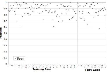
Figure 3-8 Span across Training/Test Sets ...95

Figure 3-9 Comparison of CHUNNEL and HOLE ...96

Figure 3-10 Radius Change along Porin Paths...99

Figure 3-11 Porin Paths ... 101

Figure 3-12 Residue Enrichment for Porins ... 102

Figure 3-13 The 5 Paths in Aquaporin ... 104

Figure 3-14 Residue Enrichment of Transmembrane Paths in OPM...107

Figure 3-15 Residue Enrichment in Alpha Helical OPM ... 109

Figure 3-16 Residue Enrichment in Beta Barrel OPM... 110

Figure 3-17 Paths in a Complicated Membrane Protein ... 112

Figure 3-18 Residue Enrichment for Branched Side Tunnels ... 114

Figure 4-1 Packing in Hyperthermostable Proteins ... 131

Figure 4-2 Interatomic Distances in Hyperthermostable Proteins... 135

Figure 4-3 Wadell Sphericity in Hyperthermostable Proteins ... 136

Figure 4-4 Travel Depth in Thermostable Proteins... 138

Figure 4-5 Size-Scaled Travel Depth in Thermostable Proteins ... 139

Figure 4-6 Burial Depth in Hyperthermostable Proteins... 141

Figure 4-7 Example Structure Pair Colored by Travel Depth and Burial Depth ... 142

Figure 4-8 Size-Scaled Travel Depth for the Larger Hyperthermostable Set ... 144

Figure 4-9 Residue Specific Burial Depth in Thermostable Proteins ... 146

Figure 4-10 Histogram of Burial Depth of Alanine... 148

Figure 4-11 Equal Wadell Sphericity, Different Travel Depth and Burial Depth Example ... 153

Figure 5-1 Pockets Example... 167

(16)

Figure 5-3 Pocket Finding Comparison ... 188

Figure 5-4 Pocket Finding Comparison – Binding Sites and Mouths ... 190

Figure 5-5 Adenylate Kinase Transition Visualization ... 192

Figure 5-6 Adenylate Kinase Transition Properties... 194

Figure 5-7 Adenylate Kinase Heatmap... 195

Figure 5-8 !-lactamase comparisons... 201

Figure 5-9 Protein Tyrosine Phosphatome Non-transmembrane Domain Comparison... 210

Figure 5-10 Protein Tyrosine Phosphatome Receptor Comparison... 213

(17)

Chapter 1 Introduction

The amazing property of macromolecules, especially proteins, is that they form

precise three dimensional structures by folding. These three dimensional structures

are the active forms which perform all the necessary biochemistry to maintain life in

all forms. These structures have a specific shape, which along with other properties

like charge determine the specific activity and function of each protein. This thesis

examines new methods of analyzing the shape of these macromolecules and the

results obtained from such methods.

Atomic Radii and Macromolecular Surfaces

There is a rich history of treating atoms as spheres and constructing surface models

that model the solute/solvent boundary in structural biology. The van der Waals

radius of an atom is a model that allows the size of atoms or molecules to be

understood in terms of spheres that cannot overlap due to steric constraints. The

intermolecular force that leads to this radius was postulated by Johannes Diderik van

der Waals when he developed a model that showed liquids and gases could be made

of the same matter, given that molecules existed and they had this finite size and

some attraction to each other 1; 2_{. For all work done in this thesis, the radii of the}

atoms involved (mainly the heavy atoms in biological molecules: carbon, nitrogen,

(18)

gas kinetic properties and critical densities and packing among other desirable

properties 3_.

The van der Waals radii are used to represent a macromolecule as a set of

overlapping spheres in their specific position determined by how the macromolecule

is folded. By choosing a probe to represent solvent, commonly sized between 1.2Å

and 1.8Å, a surface can be constructed that represents the boundary between solute

and solvent. The surface can be constructed from the center of the probe sphere, as

it moves as close as possible to the macromolecule (the solvent accessible surface),

or it can be constructed from the front of probe sphere (the molecular surface). An

early review on the subject of these surfaces and the areas and volumes is by

Richards 4_{. Many other advances in surface generation and analysis have been}

forthcoming5; 6; 7; 8; 9; 10; 11; 12_{. As the probe radius varies, the position of normal}

protein atoms leads to a fractal surface 13_{. Using these surfaces to analyze}

protein-water interactions has been reviewed by Levitt and Park 14_{and Raschke}15_{. Overall,}

any new analysis must be automated and fast to analyze the genomic scale data now

present in the Protein Data Bank 16_.

(19)

little other work has been done owing to the complicated algorithmic nature of the

problem. The distance of each atom to the surface is the simplest to implement, as

there are no disallowed regions and it can be computed trivially by comparing the

distance of each atom center to all surface atoms.

In this thesis, various different distances from and to this molecular surface are

computed, using a grid representation and Dijkstra’s shortest paths algorithm 23_to

approximate the distances. This allows computation of the distance of the molecular

surface from the convex hull while avoiding the molecular interior, a useful

construction that allows computation of what is called Travel Depth throughout this

work. This allows for the first time the depth of pockets on the protein surface to be

computed. Also, the distance of each atom from the molecular surface can be

computed within this framework. Finally, the distance from the molecular surface

into solvent can be computed, leaving ridges of maximal distance in the solvent that

can be exploited along with topological guidance to find tunnels all the way through

these surfaces.

In the rest of this introduction, some background on the computational geometry

and graph theory techniques used is given, followed by some background on the

various application areas to be examined along with a brief preview of the methods

(20)

Computational Geometry and Graph Theory

The exact methods of constructing surfaces used for this work uses one of two

methods, either a gaussian approximation method designed to mimic the reentrant

molecular surface24_{or a variation of the inkblot algorithm that colors grid points}

within the van der Waals plus probe radius and then erases those within the probe

radius of the surface to model the reentrant probe surface. Both methods use a grid

spaced at a resolution, typically 1Å, and produce a fully triangulated surface,

something which not all methods do. The various algorithms present here work on

these triangulated surfaces and their underlying grids, however the algorithms could

be modified to run on any triangulated surface by imposing a grid or other structure

to represent the volume.

In several algorithms used here, the convex hull surface of this molecular surface is

also calculated. In three dimensions, the Qhull code, which is algorithmically optimal

and also very fast in practice, 25_{was used. The convex hull is the smallest surface}

with no invaginations or dimples that encloses the underlying surface or point set. In

two dimensions it can be visualized by wrapping a rubberband around a set of

(21)

this is unnecessary. From here, the algorithm proceeds to compute the shortest

paths from the initiation set to all other allowed points 23_{. This is accomplished by}

using one data structure that holds the list of unseen points and another that is the

tree of connections already made. The exact nature of these data structures changes

the computational complexity of the algorithm but does not affect the results, for

review see relevant chapters of the text of Cormen et al 28_{. By keeping track of the}

closest points not yet seen and adding the closest point, the algorithm runs until all

points have been seen or the termination surface has been reached. Since this

problem has optimal subproblems, that is the shortest distance from A to C that

passes through B is the shortest distance from A to B added to the distance from B

to C, this algorithm can be completed quickly in terms of computational complexity

as well as real computer time. This algorithm is referred to as multiple source

shortest paths, Dijkstra’s shortest paths or just shortest paths.

Note that the general problem of computing shortest paths in three dimensions with

obstacles has been shown to be NP-hard 29_{, in other words it is likely that no}

polynomial time solution exists as it would mean polynomial time solutions exist to

many other common problems thought to be exponential. However, as the

construction of this proof involves creating obstacles of very fine complexity, we

avoid this lower bound since proteins, while fractal in nature, have obstacles of a

(22)

Surface Depth

Many features of macromolecules are often referred to as deep or shallow. Grooves

in DNA are often referred to as deeper or shallower and qualitative depths were

assigned to the various canonical forms 30; 3132_{. No quantitative measure of this}

depth existed. Also, many binding sites in enzymes are called deep, or binding sites

of protein-protein interactions are called shallow, again this qualitative description

had little physical meaning and no quantitative method.

Chapter 2 is a description of the algorithm invented to quantitatively measure the

depth of the protein surface including that of pockets, grooves and even tunnels.

Briefly, this involves computing the distance from the convex hull to the

macromolecular surface, while avoiding the molecule interior. This algorithm

measures the depth to all points on the molecular surface and the entire

intermediate volume between the molecular surface and the convex hull. Several

applications are included, for instance examining a large set of protein-ligand

co-crystal structures with experimental binding affinity data 33; 34_{. Understanding the}

structural features of binding sites is important for many reasons. The structural

(23)

Concurrent with this work on Travel Depth, a procedure to compute distances from a

point of interest to the convex hull was published, called CAVER 36_{. This procedure is}

different in several ways, first it requires the user to input a point of interest from

which the distance to the convex hull is calculated. Second, surfaces are not

explicitly constructed, instead a modified shortest paths algorithm finds the path that

passes as far from the atoms as possible on the way to the convex hull. This

procedure does not compute the distance to all surface and intermediate volume

points, and cannot aid in visualization of the surface by coloring according to depth.

Finally, no genomic scale analysis was completed. Any analysis possible with CAVER

is possible with Travel depth, however the inverse is not true.

Ion Channels and Pores

Ion channels and pores are membrane spanning proteins that allow substrates to

pass from one side of the membrane to the other. The process of membrane

transport is extremely important biologically, and is involved in many processes like

nutrient import or signaling. Though progress in determining their structures is

behind that of soluble proteins, the number of structures is rising at similar rates

now 37; 38_{, and numbers more than 200.}

Finding the holes that allow these substrates to pass presents a challenge

computational task even once the structure is known. Some ions are very small,

smaller than the heavy atoms that make up the proteins themselves. These tunnels

often vary in diameter as they pass through the membrane, for instance they usually

(24)

only one type of ion to pass through. These paths may not follow a straight line,

though the original potassium channel structure does 39_.

The previous work on finding and analyzing these holes is called HOLE 40; 41_{. HOLE}

needs a starting point and direction, but proceeds from there by finding the largest

circle that can be placed in each z-slice through the protein in the direction given.

This procedure works well when very small steps are taken and when the starting

point and direction are given correctly. However, it cannot identify paths that take a

winding route and cannot deal with bifurcated paths. Also, it will attempt to identify a

hole in the protein even when none exists, no topological checking is done to ensure

that each path is through a hole.

In Chapter 3, the method called CHUNNEL is presented. The first step in CHUNNEL is

to measure the shortest distance from the protein surface to all solvent points, which

leaves a maximal ridge in three dimensions near the centers of all tunnels. This is

combined with several topological procedures to guide the hole finding procedure

and ensure that each hole is actually a hole and that each hole found is topologically

distinct from all others found. This procedure works for all holes regardless of the

(25)

Concurrent with CHUNNEL, several other methods were published and are discussed

here. MOLE 44_{is an extension of CAVER}36_{, which again computes distances from a}

point of interest provided by the user to the convex hull, along a path optimized to

be far from the atoms. Instead of using a grid as before, the new path points are at

Voronoi vertices 45_{created from the protein atoms. Again, user input is required and}

no topology checking is completed, so paths are not guaranteed to be topologically

distinct. MolAxis is similar in approach in that it uses Voronoi vertices instead of grid

points, but again, user input is required to find the paths and no topological checks

are done on paths found to ensure that they are tunnels46_{. Neither of these methods}

can perform the fully automatic analysis enabled by CHUNNEL, neither are run on

the entire set of transmembrane protein structures for instance, neither find the

complete set of topologically distinct holes.

Using Voronoi vertices created from atom centers is however an interesting

technique. Since a Voronoi edge exists where any three atom centers are

equidistant, an edge will be present throughout the length of any tunnel, connecting

Voronoi vertices of atoms lining the tunnel. This seems possibly superior to using

grid points, as very fine grids may be necessary to find the smallest tunnels of

interest, for instance chloride channels. Combining the Voronoi methods with the

methods to compute the distance from the surface into solvent and topological

checking would likely be the a good combination approach, and is discussed in

(26)

Thermostability

The structural basis for thermostability of protein structures has been examined from

many perspectives. Proteins from hyperthermophilic organisms maintain their

stability even at temperatures as high as 80 degrees C. Understanding the structural

basis for thermostability is important due to the many applications like protein

design47_{. Examinations of the differences between these structures and those from}

mesophiles have commonly included analyzing the differences in exposed surface

area 48; 49; 50; 51; 52; 53; 54; 55_{. However, few if any studies have examined the}

distribution of residue burial, or distance from the atoms to the molecular surface.

Also, no study had examined the number or depth of pockets, or more generally, the

overall shape differences between hyperthermostable proteins and mesostable

homologues.

Both Burial Depth, the distance of each atom to the molecular surface, and Travel

Depth, the distance of the molecular surface from the convex hull avoiding the

protein interior, were used to analyze a dataset of thermostable and mesostable

pairs of proteins 51_{. These analyses are presented in Chapter 4, leading to the}

(27)

many applications where a good pocket definition is necessary. The field of functional

site location, similarity between sites and docking ligands into those sites is reviewed

by Campbell et al 58_.

In Chapter 5 the CLIPPERS method is introduced. Building on top of the Travel

Depth analysis, CLIPPERS analyzes all pockets on the protein surface, using a very

liberal definiton of pocket, which generates a hierarchy of nested pockets that

completely cover the protein surface. After finding pockets, their shape features are

easily computed, and pockets can then be compared and clustered. Pockets can be

tracked throughout transition pathways with time, across mutations, with different

binding partners, or across diverse families of protein structures. This work will be

published as all other work in this thesis has been59_{. There are many other pocket}

finding methods, reviewed in Chapter 4, however CLIPPERS is the first to completely

cover the protein surface with pockets and also to compare them based on shape

alone, not alignments or by residues.

Summary

By using the shortest paths method on geometric graphs, distances between

surfaces and/or volumes can be easily quantified. These distances, along with other

techniques, allow algorithms that can measure the depth of an entire

macromolecular surface, or the depth of all the atoms within the surface. Also, these

distances form the basis for methods to automatically catalog and measure both

(28)

applications, all made possible through consistent application of the shortest paths

(29)

Chapter 2

The bulk of this chapter was previously published 35_.

Summary

Depth is a term frequently applied to the shape and surface of macromolecules,

describing for example the grooves in deoxyribonucleic acid (DNA), the shape of an

enzyme active site, or the binding site for a small molecule in a protein. Yet depth is

a difficult property to define rigorously in a macromolecule, and few computational

tools exist to quantify this notion, to visualize it, or analyze the results. We present

our notion of travel depth, simply put the physical distance a solvent molecule would

have to travel from a surface point to a suitably defined reference surface. To define

the reference surface, we use the limiting form of the molecular surface with

increasing probe size: the convex hull. We then present a fast, robust approximation

algorithm to compute travel depth to every surface point. The travel depth is useful

because it works for pockets of any size and complexity. It also works for two

interesting special cases. First, it works on the grooves in DNA, which are unbounded

in one direction. Second, it works on the case of tunnels, that is pockets which have

no 'bottom', but go through the entire macromolecule. Our algorithm makes it

straightforward to quantify discussions of depth when analyzing structures.

High-throughput analysis of macromolecule depth is also enabled by our algorithm. This is

demonstrated by analyzing a database of protein-small molecule binding pockets,

(30)

show significant, but subtle effects of depth on ligand binding localization and

strength.

Introduction

Depth is a term frequently applied to the shape and surface of macromolecules. For

example, enzyme active sites are routinely described as shallow or deep. Small

ligand binding sites on proteins are also frequently described in term of depth. Depth

is just one facet of the property 'binding pocket shape' one would like to define

quantitatively, to aid for example, in screening a large library of potential ligands, or

in docking of a candidate ligand. Groove depth is one of the fundamental terms used

to describe the differences in structure of the A, B and Z forms of DNA 30; 31; 60_{. In}

spite of the common use of the term depth, it is a surprisingly difficult property to

define rigorously in a macromolecule. Discussions of depth in the literature, although

intuitively reasonable, are usually qualitative. The concept of depth is thus difficult to

subject to rigorous analysis or to extract the most information from. A large part of

the difficulty in analyzing depth is due to the complexity and range of shapes

adopted by macromolecules. Protein surfaces are fractal in nature 13_{, adding to the}

(31)

bottom of the pocket to the nearest surface, while easy to define and compute, will

be a very misleading and grossly underestimating measure of depth. These

difficulties are reflected in the fact that there are few computational tools to quantify

the concept of depth, to visualize it, or analyze the results. To address this problem,

we present here our notion of travel depth, simply put the physical distance a

solvent molecule would have to travel from a surface point to a suitably defined

reference surface. The concept of travel depth was designed to avoid the 'short

circuiting' error described above, and also to solve the problem of a reference level.

We first define the concept of travel depth, and the reference level used by it, then

present a fast, robust approximation algorithm to compute travel depth to every

surface point. Selected examples using very different molecular shapes are used to

demonstrate that our definition of depth works for special cases, and that it conforms

to our intuition, so confirming that we have introduced a 'good' definition for depth

and that our approximate numerical implementation of it is reasonable. We then

describe some applications of our algorithm, including a high throughput application

to a small molecule binding database.

Theory and Methods

Definition of travel depth

Any measure of depth must start with the questions: Depth of what, and from what?

In this work, we are concerned with the depth of any point on the molecule's

surface. Two definitions of surface predominate for macromolecules, the solvent

(32)

the probe radius, which is almost universally taken to be that of water (usually

values between 1.4Å and 1.8Å are used). Many algorithms exist for computing these

idealized surfaces. Most, but not all, produce a triangulated form of the surface,

primarily for display using standard computer graphic routines 10; 12; 24; 61_{. Our}

algorithm assumes a simple closed triangulated surface. The surface must be

orientable and connected, though these are not strong requirements; The latter

disallows only cavities. For the broadest applicability of our method, we make no

other assumption about how the surface was produced, or what it should look like. In

practice we use the molecular surface as generated by the algorithm in the GRASP

macromolecular graphics program 24_{implemented as a stand-alone program}62_using

a probe radius of 1.8Å and standard atomic radii 3_{. Though we test only this surface}

generation scheme and the resulting triangulated surfaces, our definition and

algorithm generalize to any triangulated surface generation scheme.

Our definition of travel depth is that for each point on the molecular surface, the

travel depth is the minimum distance a solvent probe would have to travel through

the solvent from that surface point to get to the reference level. A natural and

parameter independent reference level is provided by the convex hull of the

(33)

The next step is to compute the minimal distance from every surface point to the

convex hull while respecting the boundary of the molecular surface. In other words,

the travel path along which the distance is computed must lie outside the molecular

surface in the solvent. We note that computing such a minimal distance between two

points while avoiding obstacles is exactly the shortest path planning problem

commonly encountered in robotics, and that an exact solution to the problem is

NP-hard. Our solution, described below, is to approximate this minimal distance in such

a way that it was easy to code and run in a short time so that we could establish

what the depth measure would look like on real examples, and whether it would be

useful in structural analysis.

Calculation of travel depth: Preprocessing

The first step is to remove cavities, defined as completely enclosed solvent pockets

in the molecular surface. The triangles that represent these cavities are removed

from the surface and are not used in later calculations. Since there is no way for the

solvent probe to travel from a closed cavity surface to the convex hull without

passing through the macromolecule itself, travel depth does not apply to these

surfaces. We note, though, that simple Euclidean distance to the nearest part of the

external molecular surface would provide a satisfactory definition of the minimum

depth of a closed cavity.

Two important pre-processing steps are done at this stage. First, the longest edge of

any triangle in the surface is found and the length saved for later. Also, all the points

(34)

structure oriented along one grid axis 26_{. This helps improve the running time, as}

described later, but it is non-essential to the algorithm.

Calculation of travel depth: Mapping onto Grid

The macromolecule and a region of the surrounding solvent are embedded in a cubic

grid of dimensions K x L x M. For convenience, the grid extends to one grid cube

beyond the minimum and maximum coordinate of the molecular surface in each

orthogonal direction, so that the border is completely outside the surface. The

default grid spacing used in our algorithm is 1Å, however the algorithm and code

generalize to any spacing. The only consideration is for the spacing to be small

enough to approximate well the topology of the given molecular surface. For

instance, when a probe radius P=1.8Å is used, as in our surfaces, the maximum

concavity of any section of the molecular surface is limited to that of the probe

radius. From this, a maximum allowable grid spacing, G, can be calculated from the

formula

!

G

=

2P

3

(2-1)

(35)

1.4Å). This assumption ignores problems caused by a very coarse surface, though

this assumption is relaxed and a solution to problems caused by this in our algorithm

are discussed later.

The next step of the algorithm is to find the convex hull of the molecular surface.

There are many O(n log n) algorithms for computing the convex hull in three

dimensions. We use available code from Qhull or Quickhull, an optimized and robust

package 25_.

Calculation of travel depth: Classifying Grid Points

After construction of the convex hull each point lying at the center of each grid cube

must be checked to see whether it lies inside or outside the convex hull and inside or

outside the molecular surface. The convex hull can be represented as a list of

outward facing triangles. A sufficient check for being outside the convex hull is to

check the point against each triangle and surface normal to see which side it is on. A

point that is outside any convex hull triangle is outside the entire convex hull. Doing

this check for each point in the grid is sufficient to determine which points are

outside the convex hull and which are inside. Next, points inside the convex hull are

assigned to either the outside or the inside of the molecular surface. This step is the

most time consuming portion of the entire algorithm. The problem is that

determining whether a point is inside or outside a general triangulated surface

requires global information. It is not sufficient to check a point against every surface

triangle. However, an appropriate geometric property can be used to solve this

(36)

will intersect an even number of triangles. Lines are constructed in one orthogonal

direction of the grid such that they each pass through a set of grid points. Moving

from grid point to grid point along this line from one side of the grid until the first

triangle is met assigns all those points to the outside. Each time a triangle is

encountered, the inside/outside assignment switches. This procedure is continued

until the opposite side of the grid is reached. In this manner, when a complete set of

lines through the grid in one direction have been processed, the correct assignment

has been made for all the points. In practice, since a line of grid points is used in this

step, all their inside or outside checks can be done at once: Each triangle from the

surface can be checked to see if it intersects this line, and to find the point of

intersection if it exists. After this, the previously described procedure can be used to

determine on which side of the surface each point on that line lies.

Naïvely, each triangle could be tested against each line. However, a more efficient

procedure which drastically cuts down the number of intersection checks uses both

of the preprocessing steps mentioned earlier. After picking a dimension along which

the lines will be constructed, the other two dimensions are chosen as the orthogonal

directions to construct a 2 dimensional orthogonal range search tree from all the

(37)

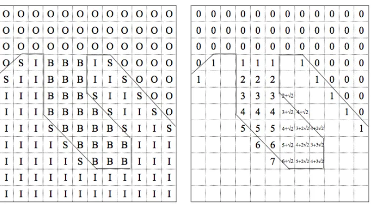
Figure 2-1 Travel Depth 2D example

Two schematic two-dimensional examples of the Travel Depth Algorithm. Left: an

example of a piece of a macromolecule, the grid superimposed on it, and class

assignments made: outside convex hull (class O), inside the molecular surface but

containing at least one molecular surface point (class S), inside molecular surface

and not containing any molecular surface points (class I), and between the convex

hull and molecular surface (class B). Right: the travel depths assigned to each grid

(38)

test quickly reduces the number of triangle intersection checks that must be done.

Though these checks each take constant time, they can be very slow, as they involve

evaluating several matrix determinants. To unambiguously determine inside and

outside, our algorithm assumes that these lines will not intersect a triangle across its

face, or through a single vertex. These special cases, if they occur, are easy to

detect and the points can be slightly perturbed until the ambiguity no longer occur.

At this point each grid cube has been classified into one of four categories based on

the location of its center and whether it contains any molecular surface points. Either

outside the convex hull (class O), between the convex hull and molecular surface

(class B), inside the molecular surface but containing a molecular surface point (class

S) or finally inside the molecular surface but containing no molecular surface points

(class I). A small example is shown in the left panel of Figure 2-1. Class I cubes are

ignored in the rest of this work, as no depth needs to be calculated for them.

Calculation of travel depth: Assignment of Travel Depth to Grid Points

It remains to approximate the minimum distance that a probe sphere would need to

travel to get from each surface point to the convex hull. This travel depth is assigned

(39)

assigned depth, which is usually the case, the neighbor that results in the minimum

depth di is chosen. Symbolically.

!

d

_i

=

j

min(

d

_j

+

dist

(

i

,

j

))

(2-2)

where j ranges over all neighbors of i. This procedure is repeated until no new depth

assignments are made.

A key requirement to correctly propagate depth with respect to the topology of the

molecular surface is the appropriate definition of neighboring cubes in equation 2-2.

For a class O or B cube, any of the 26 immediately adjacent cubes of class O, B or S

are considered neighbors. Additionally molecular surface edges which have an

endpoint in a class O or B cube and another endpoint in a class O, B, or S cube make

those two cubes neighbors. For class S grid cubes, any adjacent cube of class O or B

is a neighbor. However, for a class S cube only class S grid cubes that are connected

to it by a molecular surface edge are considered neighbors, even if the two S class

cubes are adjacent. There may be adjacent class S grid cubes that do not have a

molecular surface edge between them, for example when two distant parts of the

molecular surface approach each other very closely without meeting. It is important

not to propagate the travel depth across this gap.

The neighbor distances in equation 2-2 are defined as follows: Each grid cube has 6

adjacent cubes that share one face, 12 adjacent cubes that share only an edge and 8

adjacent cubes that share only a vertex. The distances to these three types of

(40)

units respectively. Additionally, cubes of class S can have additional neighbors

defined by edges of the molecular surface which have endpoints in the two grid

cubes, i and j. Their distance is also the Euclidean distance between the grid cube

centers.

Starting from the class O grid cubes with depth 0, the neighboring grid cubes are

assigned a depth according to equation 2-2, then the neighbors of the neighbors are

assigned and so on. In this way the depth propagates in towards the molecular

surface, and into the class S cubes, but it does not propagate through the

macromolecule since the depth assignment is not propagated into class I cubes. This

is illustrated in the right panel of Figure 2-1. After the assignment phase terminates,

the depth is converted from grid units into a physical distance by multiplying by the

grid spacing. This results in a calculation of the shortest paths from the class O cubes

to all class B and class S cubes, given the neighbor and distance definitions above.

The depth assignment phase of the algorithm is speeded up by using Dijkstra’s

algorithm for shortest paths on a graph 28_{and using available code that implements}

a key component of that algorithm, a priority heap. Dijkstra’s algorithm keeps track

(41)

At this stage, all that remains is to assign each surface point a depth based on the

grid cube it is located in, resulting in a computed travel depth for each point on the

surface. The travel depth is also computed for all the grid cubes B between the

molecular surface and the convex hull as well as the grid cubes I that contain surface

points. Although the travel depth assignment of points between the convex hull and

the molecular surface is not used in the applications of travel depth described here, it

is a property that may prove useful in future applications like docking.

Presentation of results

To visualize the results of our algorithm we used the macromolecular graphics

package PyMOL 64_{. The triangulated molecular surface can easily be read into this}

program, along with travel depth values, and a red-green-blue color gradient

assigned to each point of the surface based on travel depth. Red represents a travel

depth of zero, with increasing depth indicated as the color changes from green to

blue. The depth represented by blue is set either to the maximum value for that

molecule, or to a fixed value to compare of a set of molecules. Color values at each

point along each edge and triangle are interpolated using the standard approach to

produce a smooth visualization of depth 64; 65_{. Further refinements, such as}

displaying only surface in a certain range of depth may be useful for particular

applications, and are straightforward with our algorithm.

Robustness, errors and timing analysis

Depending on the size of the macromolecule and the resolution at which the

(42)

be quite coarse. In this case regions of the surface may not conform well to the

estimates of maximum concavity. This may result in small crevices or tunnels which

violate the maximum concavity assumption. These errors are accounted for by the

molecular surface edges that define grid cube adjacencies. The only level of

coarseness that may cause a problem is where two parts of the surface approach

each other very closely, less than the grid spacing. In these cases, the travel depth

would propagate between these surfaces when it should not. However, to violate this

assumption requires a violation of the maximum convexity assumption, which

corresponds to a severe underestimation of the size of an atom or adjacent atoms

forming such a barrier.

There are two sources of error in our approximation algorithm, each of which can be

reduced at the cost of increasing the running time of the algorithm. The first source

of error comes from the grid orientation. The approximate distance can be

overestimated if a significant part of the path traveled is diagonal with respect to the

grid axes. The worst case is when the actual distance should be down two grid units

and over one grid unit in both other directions, the path length here is !6, while the

approximation given is 1 grid unit down and then one diagonal step of length !3.

(43)

The second source of error lies in the discretization of the distance, again from the

use of the grid cubes to approximate the distance. Using smaller grid cubes, at a

cost of increasing the running time, can reduce this error. In practice, there is little

reason to get an extremely accurate measure of this distance, as there are already

sources of uncertainty regarding the travel depth property, and indeed in the

molecular surface construct itself. It would be hard to argue that differences of some

small travel depth distance like 1Å had any real physical meaning.

Our algorithm has both a reasonable asymptotic running time when the complexity is

analyzed, and a reasonable running time in practice. Also, following the philosophy of

keeping the code as simple as possible, time spent coding and debugging was

minimized, available pieces of code like PyMOL 64_{and a priority heap}63_{were used}

when possible.

We have highlighted the practical runtime issues throughout the description of the

algorithm. The algorithm also has a reasonable running time when analyzed

asymptotically 28_{. Without the orthogonal range search tree speedup mentioned, the}

running time is

(2-3)

where p is the number of points on the molecular surface, c is the number of

triangles on the convex hull, t is the number of triangles on the molecular surface, d

is the number of grid cubes in any dimension, and e is the number of edges, which is

!

O p

log

p

+

cd

3

+

(

t

+

d

)

d

2

+

(

d

3

+

e

)log

d

3

(44)

linear in terms of t and d3_{. The first term in equation 2-3 comes from the convex hull}

construction, the second term from the checks for each grid cube to see if it is inside

or outside the convex hull. The third term comes from the checks to see if each grid

cube is inside or outside the molecular surface. The fourth term is the cost of the

propagation step using the shortest path algorithm and amortized time cost priority

heap.

With the orthogonal range search tree speedup in place, there are two additional

components to consider, the O(t) steps to find the longest triangle edge, the O(t log

t) steps to build the orthogonal range search tree (faster algorithms exist, but are

harder to code 26_{). The}_O((t+d)d2₎_{term to check each grid cube becomes}_O((log2_(t)

+ k + d)d2₎_{step to do a range search query and then}_k_{checks must be done, where}

k is the number of triangles returned from the range search. Also, it should be noted

as was later revealed by our timing analysis that the orthogonal range search idea

should probably be applied to the inside/outside convex hull routine, changing the

O(cd3₎_{time into}_{O(c log c + ((log}2_{(c) + d)d}2₎₎_{as the time for the convex hull checks}

now outweighs the time for the molecular surface checks as we have it implemented.

(45)

factor k representing how many triangles are returned from an average range

query. Though an initial penalty must be paid, this provides an overall faster

approach as the number of triangles increases. This allows us to use very fine

triangulated surfaces and still maintain reasonable runtimes, or use very coarse

triangulated surfaces to get good exploratory results.

To give some estimate of the processing time involved, we provide the following

timing analysis, conducted using one processor of a dual processor machine (Intel

2.4 GHz chip, 4797 BogoMIPS, 1 gigabyte RAM) running RedHat Linux 9.0. Different

parts of the algorithm were timed separately. Two test PDB files were used, s a

representative small protein, cyclic bovine pancreatic trypsin inhibitor, PDB code

1K6U. To represent larger more complicated proteins, the 6 chain biological unit of

pertussis toxin was used, taken from PDB code 1PRT. For these two samples we

constructed molecular surfaces of varying fineness, the number of triangles in each

is reported, along with times in seconds for each of the three main phases of our

algorithm. All these results are shown in Table 2-1. It should be noted that while the

orthogonal range search tree speedup was in place for the molecular surface, it was

not in place for the convex hull code here.

We note that during even the largest test case examined, only about 200 megabytes

of available memory were in use, suggesting that memory usage is not a limiting

factor in our algorithm, even though no formal asymptotic space analysis was

conducted. The runtime for the large example at fine granularity represents an

(46)

Table 2-1 Timing analysis of travel depth code

PDB Code 1K6U 1PRT

Level of Detail coarse medium fine coarse medium fine

Number of Triangles 3644 8148 30896 5940 13780 57836

Inside/outside

Convex Hull (s) 14 21 53 14 241 443

Inside/outside

Molecular Surface (s) 4 5 12 5 48 153

Depth Assignment(s) 9 10 15 9 126 149

(47)

statistical analyses were done at a more medium granularity setting, which proved

sufficient.

Results

The first tests of the travel depth algorithm were designed to see if the definition

conformed to one’s qualitative intuition about depth in macromolecules. In other

words, is the definition of travel depth reasonable and useful? We used a variety of

structures that had qualitatively different surface topographies. The first is duplex

DNA, to which the term groove depth is commonly applied. We evaluated the depth

of the major and minor grooves in A, B and Z canonical forms of DNA. 15 base pairs

of A-T were generated with the routine NUCGEN 66_{in canonical A form, crystal}

structures 1BNA67_{and 3ZNA}32; 68_{were used for the B and Z forms respectively. It}

should be noted the structure 3ZNA was constructed by duplicating base pairs

present in the crystal to achieve the length shown, and is therefore considered a

theoretical model in the PDB. Our travel depth algorithm gives intuitively reasonable

results, shown in Figure 2-2. All surfaces are colored from red (travel depth 0 Å) to

green (travel depth 7 Å), then finally to blue (travel depth 14 Å). It is clear that the

major and minor grooves of the B-form are nearly the same depth, whereas the

major groove of the A-form is much deeper than the minor groove of A-form or

either groove of the B-form. Also, what would usually be the minor groove has

turned into a very deep groove in the Z-form, and the major groove has almost no

depth. We summarize these results quantitatively in Table 2-2. This is in good

agreement with the standard description of these grooves 30; 31; 60_{. Specifically, “in}

(48)

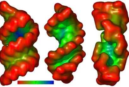
Figure 2-2 Travel Depth of DNA

Travel Depth coded molecular surface of the three canonical forms of DNA, from left

to right, A, B, and Z. All surfaces are colored from red (travel depth 0Å) to green

(travel depth 7 Å), then finally to blue (travel depth 14 Å) as indicated by the color

(49)

Table 2-2 Travel Depths of Selected Macromolecular Featuresa Major Groove Max Depth Minor Groove Max Depth Major Groove Average Depth Minor Groove Average Depth

A-DNA 13.7 5.0 8.6 3.6

B-DNA 10.0 9.1 4.6 5.6

Z-DNA 4.2 10.8 2.0 6.5

Binding Site Average Depth Binding Site Max Depth Tunnel Depth at Center Ring Around Tunnel Depth

Tunnel (1A0Q) 10.6 18.0 23.0 18.0

Horseradish Peroxidase

(1ATJ) 18.8 24.0

Streptavidin-Biotin

(1MK5) 8.5 10.0

(50)

Figure 2-3 Travel Depth of Streptavidin

An example binding pocket color coded by travel depth. This example is PDB code

1MK5, a biotin/streptavidin complex, the biotin binding site has a maximum travel

(51)

groove very deep, the minor groove shallow…” 30_{. Also, B-DNA is described: “This}

means that major and minor grooves are of comparable depth…” 30_{. Finally, Z-DNA is}

described: “With the helix axis passing down the minor groove, that groove is

extremely deep, whereas the major-groove edge of each base pair is pushed out to

the perimeter of the helix, giving the groove zero depth” 30_.

To further illustrate that our algorithm is intuitively correct, we show three other

examples. First, a simple well-known pocket was analyzed, that of streptavidin

bound to biotin (PDB code 1MK5). The result is shown in Figure 2-3. This clearly

illustrates that travel depth can quantitate a pocket near the surface. Next, a tunnel

is shown in Figure 2-4 from the FAB fragment (PDB code 1A0Q 69_{). The travel depth}

algorithm works well in this case. Despite the fact the tunnel has no bottom the

middle of the tunnel is correctly identified as the deepest point. Also, the tunnel in

Figure 2-4 is additionally characterized by the maximum distance for which a solid

connected ring of surface points exists all the way around the tunnel, which is 18 Å.

Finally, horseradish peroxidase (PDB code 1ATJ) is shown, which has a very deep

active site. Figure 2-5 shows the result, which illustrates a case where a purely

Euclidean distance algorithm would fail, as the deepest part of the pocket is closer to

the other side of the protein than the one the substrate must enter from. A summary

of various features on these previous six examples is shown in Table 2-2.

As an example of a high throughput data base application of the travel depth

algorithm, we examined the small molecule binding structural database PDBbind 33;

34_{. All 900 structures were used from the 2003 refined set}34_{. The proteins each bind}

(52)

(53)

Figure 2-4 Travel Depth on a Tunnel

(Preceeding Page) An example tunnel color coded by travel depth. This is a FAB

fragment from PDB code 1A0Q. The top view looks down on the tunnel, the bottom

view is a side view that has been cutaway through the tunnel.

Figure 2-5 Travel Depth on a Deep Pocket

(Following Page) An example deep pocket color coded by travel depth. Two views of

horseradish peroxidase, taken from PDB code 1ATJ. The bottom view is a cutaway

showing one view of the pocket with a maximum depth near the ligand of 24 Å . A

straight line Euclidean metric from the deepest point of this pocket would travel

(54)

(55)

as well as separate files for protein and ligand. Binding data for this set is from either

the dissociation constant ( –log Kd) or competitive inhibitor concentration (- log Ki),

both referred to here for brevity as –log K. This database was chosen over other

available options because the structures and binding data had been hand checked

and gathered from original sources, and the structure files were easily accessible,

downloadable in modified, in clean form within one archive file. This allowed us to

perform the analysis with only minor conversion of data formats, and no further

editing or checking of input files. We note that 13 of these structures had ligands

completely enclosed in cavities, inaccessible to solvent, and therefore only 887

structures were used whenever the ligand site was analyzed. The protein atom

coordinates were used to construct the molecular surface at a medium setting of

surface coarseness. We assume that sampling the travel depth at these surface

points gives us an accurate and representative picture of the depth of the protein, or

of a ligand binding site for instance. Under this assumption, averaging the travel

depth across the surface points is an acceptable way to measure the overall travel

depth of a protein, as is done later.

To test the hypothesis that ligands are in deeper pockets rather than shallower

pockets, the protein surface points were divided into two classes, those near ligand

atoms representing the binding site, and the rest. For each atom in the ligand, the

single nearest surface point was found and included in the binding site if it was

within an arbitrary threshold of 4Å. This method gave a simple way of partitioning

the surface into the binding site and the rest of the surface, erring on the side of

(56)

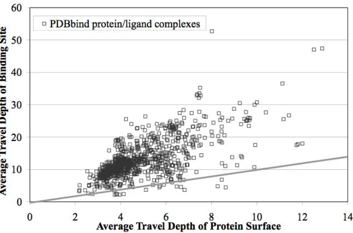
Figure 2-6 Travel Depths of Protein Surface and Binding Site

Average travel depth of entire protein surface plotted against average travel depth of

just the binding site, db for each structure in the PDBbind dataset. The y=x line is

(57)

2-6. In the figure, for each protein the average depth of the binding site surface, db,

is plotted against the average depth of non-binding site surface, dn. The vast

majority of the points lie above the x=y line indicated on the figure, demonstrating

that the binding site is almost always a pocket, as expected.

Next, the distribution of depths of ligand binding sites was compared to the

distribution of the overall surfaces, across the entire 887 complexes. For comparison,

a small control dataset with proteins not known to bind any ligands was analyzed as

well 70_{. We note that 1TGF was left out of the control dataset since it is no longer in}

the PDB. We removed the waters, ions and buffers found in these control structures

for the analysis. The histograms showing the depths of the surface points in each

category over the entire dataset are shown in Figure 2-7. The since the number of

surface points in each set is so different, the data has been normalized so that the

area under each curve is equal. The figure shows there is a clear but not complete

preference for deeper points to be near a ligand binding site. Interestingly, the width

of the histogram for proteins that bind a ligand is greater than that for the control,

'non-binding' proteins. This indicates that binding proteins tend to have a rougher, or

more corrugated surface. This raises the possibility that some proteins are

intrinsically more ‘bindable’ than others due to the kind of surface topography they

have.

Finally, to calculate the statistical significance that the ligands had some bias to be

near deeper surface points, a permutation p-value test was conducted. For each

protein, the complete set of surface points was assembled, including both the ligand

(58)

Figure 2-7 Travel Depth Histogram

A histogram comparing travel depths of different structure subsets: A control set

with no known ligands, the PDBbind set, and just the binding pockets of the

(59)

equal in number to those in the ligand binding site was taken, and the average depth

found. This random selection was repeated five million times. The p-value is the

number of times this selection had greater than the average depth of the true ligand

binding site db divided by the number of random sets. With five million random

permutations, the lower bound on the possible p-value is 2x10-7_{. This test gives a}

good measure of whether the ligand bound to each protein is bound in a deep pocket

more often that random. A more complete estimate would use all the potential ligand

binding sites on the surface, and calculate the average depth for each. However,

generating all the possible ligand binding sites is a rather complicated problem, one

which is usually solved by only sampling some of the possible binding sites 71; 72_.

The complete results of the permutation tests on the PDBbind dataset are given as

Table A-1, along with the average depth of the binding site. To summarize the

results, 13 of 900 structures contained ligands that were completely enclosed in

cavities, inaccessible to the outside solvent. Excluding those in cavities, 48 of 887

structures had a p-value greater than 0.05, so the remaining 839 structures had

ligands which were in significantly deep pockets under this criteria. Under the

strictest requirement tested, that of having a p-value less than 2x10-7_{, 688 of 887}

structures had ligands buried in these significantly deep pockets.

In Figure 2-8 we examine the relationship between protein size and average surface

depth using the PDBbind data set. As a robust measure of protein size that could

easily be computed for the entire data set we used the total number of heavy atoms.

Assuming very similar packing densities for all proteins, number of heavy atoms

(60)

Figure 2-8 Travel Depth Correlated with Size

Average travel depth of the entire protein (") and just the binding site (o) plotted vs.

the cube root of the number of heavy atoms, for proteins in the PDBbind dataset.

(61)

root of the number of heavy atoms since for a largely globular set of proteins this

metric should scale well with the linear dimension of the protein. Indeed, for the

mean surface depth averaged over the entire protein surface there is an excellent

linear correlation (R2_{=0.84). Thus average depth increases linearly with protein size.}

Not surprisingly, larger proteins can have deeper pockets, but for the average depth

to increase with protein size larger proteins must also have more pockets of

significant depth, i.e. be rougher. The scaling law indicates that average travel depth

is an indicator of overall surface roughness, and a good reflection of the fractal

nature of the protein surface, as was discovered previously by analysis of surface

area13_{. The fact that the fractal nature of the protein surface also emerges from a}

quite different analysis based on depth provides additional validation of the concept

of travel depth. Looking at depth data from just the ligand binding sites, there is still

some correlation with protein size, but the significantly smaller variance in travel

depth is explained by protein size (R2_{=0.47). This may include effects from the}

smaller amount of averaging involved in using a small subset of the protein surface.

A straightforward question to answer with the binding affinity data from the PDBbind

dataset is whether binding affinity of the ligand (-log K) correlates with the average

travel depth at which the ligand is bound. A priori, one might expect deeper pockets

to have greater affinity, based on the idea that a deeper pocket would make more

interactions with the ligand. On the other hand, the amount of surface area one

could bury or interactions one could make when binding a small ligand is limited by

the ligand size. For a given amount of surface burial or number of interactions, one

(62)

Figure 2-9 Travel Depth versus Affinity

Mean ligand binding site travel depth, db, plotted against experimental binding

affinity for the PDBbind dataset. Only ligands bound significantly deep (p-value <

Shortest Geometric Paths Analysis in Structural Biology

University of Pennsylvania

ScholarlyCommons

Publicly Accessible Penn Dissertations

Winter 12-15-2009

Shortest Geometric Paths Analysis in Structural

Biology

Ryan G. Coleman

Follow this and additional works at:

http://repository.upenn.edu/edissertations

Part of the

Computational Biology Commons

,

Structural Biology Commons

, and the

Theory and

Algorithms Commons

Recommended Citation

Shortest Geometric Paths Analysis in Structural Biology

The surface of a macromolecule, such as a protein, represents the contact point of any interaction that

molecule has with solvent, ions, small molecules or other macromolecules. Analyzing the surface of

macromolecules has a rich history but analyzing the distances from this surface to other surfaces or volumes

has not been extensively explored. Many important questions can be answered quantitatively through these

analyses. These include: what is the depth of a pocket or groove on the surface? what is the overall depth of the

protein? how deeply are atoms buried from the surface? where are the tunnels in a protein? where are the

pockets and what are their shapes? A single algorithm to solve one graph problem, namely Dijkstra’s shortest

paths algorithm, forms the basis for algorithms to answer these many questions. Many distances can be

measured, for instance the distance from the convex hull to the molecular surface while avoiding the interior

of the surface is defined as Travel Depth. Alternatively, the distance from the surface to every atom can be

measured, giving a measure of the Burial Depth of given residues. Measuring the minimum distance to the

protein surface for all points in solvent, combined with topological guidance, allows tunnels to be located.

Analyzing the surface from the deepest Travel Depth upwards allows pockets to be catalogued over the entire

protein surface for additional shape analysis. Ligand binding sites in proteins are significantly deep, though

this does not affect the binding affinity. Hyperthermostable proteins have a less deep surface but bury atoms

more deeply, forming more spherical shapes than their mesophilic counterparts. Tunnels through proteins can

be identified, for the first time tunnels that are winding or bifurcated can be analyzed. Pockets can be found all

over the protein surface and these pockets can be tracked through time series, mutational series, or over

protein families. All of these results are new and for the first time provide quantitative and statistical

verification of some previous hypotheses about protein shape.

Dissertation

Doctor of Philosophy (PhD)

Genomics & Computational Biology

Acknowledgement

Table of Contents

List of Tables

List of Illustrations

Chapter 1

Introduction

Atomic Radii and Macromolecular Surfaces

Computational Geometry and Graph Theory

Surface Depth

Ion Channels and Pores

Thermostability

Summary

Chapter 2

Summary

Introduction

Theory and Methods

Definition of travel depth

!

G

=

2P

3

!

d

=

min(

d

+

dist

(

i

,

j

))

Presentation of results

Robustness, errors and timing analysis

!

O p