Exploring The Universe With The Atacama Cosmology Telescope: Polarization-Sensitive Measurements Of The Cosmic Microwave Background

(1)

University of Pennsylvania

ScholarlyCommons

Publicly Accessible Penn Dissertations

2017

Exploring The Universe With The Atacama

Cosmology Telescope: Polarization-Sensitive

Measurements Of The Cosmic Microwave

Background

Marius Lungu

University of Pennsylvania, mlungu@sas.upenn.edu

Follow this and additional works at:

https://repository.upenn.edu/edissertations

Part of the

Astrophysics and Astronomy Commons

This paper is posted at ScholarlyCommons.https://repository.upenn.edu/edissertations/2990 For more information, please contactrepository@pobox.upenn.edu.

Recommended Citation

Lungu, Marius, "Exploring The Universe With The Atacama Cosmology Telescope: Polarization-Sensitive Measurements Of The Cosmic Microwave Background" (2017).Publicly Accessible Penn Dissertations. 2990.

(2)

Exploring The Universe With The Atacama Cosmology Telescope:

Polarization-Sensitive Measurements Of The Cosmic Microwave

Background

Abstract

Over the past twenty-five years, observations of the Cosmic Microwave Background (CMB) temperature fluctuations have served as an important tool for answering some of the most fundamental questions of modern cosmology: how did the universe begin, what is it made of, and how did it evolve? More recently, measurements of the faint polarization signatures of the CMB have offered a complementary means of probing these questions, helping to shed light on the mysteries of cosmic inflation, relic neutrinos, and the nature of dark energy. A second-generation receiver for the Atacama Cosmology Telescope (ACT), the Atacama Cosmology Telescope Polarimeter (ACTPol), was designed and built to take advantage of both these cosmic signals by measuring the CMB to high precision in both temperature and polarization. The receiver features three independent sets of cryogenically cooled optics coupled to transition-edge sensor (TES) based polarimeter arrays via monolithic silicon feedhorn stacks. The three detector arrays, two operating at 149 GHz and one operating at both 97 and 149 GHz, contain over 1000 detectors each and are continuously cooled to a temperature near 100 mK by a custom-designed dilution refrigerator insert. Using ACT's six meter diameter primary mirror and diffraction limited optics, ACTPol is able to make high-fidelity measurements of the CMB at small angular scales (l ~ 9000), providing an excellent complement to Planck. The design and operation of the instrument are discussed in detail, and results from the first two years of observations are presented. The data are broadly consistent with /\CDM and help improve constraints on model extensions when combined with temperature measurements from Planck.

Degree Type

Dissertation

Degree Name

Doctor of Philosophy (PhD)

Graduate Group

Physics & Astronomy

First Advisor

Mark Devlin

Subject Categories

(3)

EXPLORING THE UNIVERSE WITH THE ATACAMA COSMOLOGY TELESCOPE: POLARIZATION-SENSITIVE MEASUREMENTS OF THE

COSMIC MICROWAVE BACKGROUND Marius Lungu

A DISSERTATION in

Physics and Astronomy

Presented to the Faculties of the University of Pennsylvania in

Partial Fulfillment of the Requirements for the Degree of Doctor of Philosophy

2017

Supervisor of Dissertation

Mark Devlin, Professor of Physics

Graduate Group Chairperson

Joshua Klein, Professor of Physics

Dissertation Committee

(4)

ABSTRACT

EXPLORING THE UNIVERSE WITH THE ATACAMA COSMOLOGY

TELESCOPE: POLARIZATION-SENSITIVE MEASUREMENTS OF THE

COSMIC MICROWAVE BACKGROUND

Marius Lungu

Mark Devlin

Over the past twenty-five years, observations of the Cosmic Microwave Background

(CMB) temperature fluctuations have served as an important tool for answering some of

the most fundamental questions of modern cosmology: how did the universe begin, what is

it made of, and how did it evolve? More recently, measurements of the faint polarization

signatures of the CMB have offered a complementary means of probing these questions,

helping to shed light on the mysteries of cosmic inflation, relic neutrinos, and the nature of

dark energy. A second-generation receiver for the Atacama Cosmology Telescope (ACT),

the Atacama Cosmology Telescope Polarimeter (ACTPol), was designed and built to take

advantage of both these cosmic signals by measuring the CMB to high precision in both

temperature and polarization. The receiver features three independent sets of cryogenically

cooled optics coupled to transition-edge sensor (TES) based polarimeter arrays via

mono-lithic silicon feedhorn stacks. The three detector arrays, two operating at 149 GHz and one

operating at both 97 and 149 GHz, contain over 1000 detectors each and are continuously

cooled to a temperature near 100 mK by a custom-designed dilution refrigerator insert.

Us-ing ACT’s six meter diameter primary mirror and diffraction limited optics, ACTPol is able

to make high-fidelity measurements of the CMB at small angular scales (` _∼ 9000),

pro-viding an excellent complement to Planck. The design and operation of the instrument are

discussed in detail, and results from the first two years of observations are presented. The

data are broadly consistent with ΛCDM and help improve constraints on model extensions

(5)

LIST OF TABLES

3.1 Estimated O-ring leak-rates for the ACTPol vacuum shell . . . 60

3.2 Nominal properties of ACTPol’s three LPE filter stacks . . . 81

3.3 Measured TES detector parameters for ACTPol’s three arrays . . . 103

4.1 Summary of two-season ACTPol D56 night-time data . . . 110

4.2 Internal consistency tests . . . 119

4.3 Null test results from custom maps . . . 129

(8)

LIST OF FIGURES

1.1 The cosmic timeline . . . 3

1.2 Slow-roll scalar field inflation . . . 12

1.3 The CMB blackbody spectrum . . . 19

1.4 Map of the primary CMB temperature anisotropies . . . 21

1.5 The CMB temperature angular power spectrum . . . 24

1.6 Quadrupole Thomson scattering . . . 26

1.7 E and B-mode polarization . . . 27

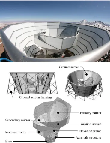
2.1 The Atacama Cosmology Telescope structure . . . 30

2.2 Optical depth and PWV at the ACT site . . . 32

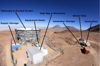
2.3 Annotated view of the ACT site . . . 34

2.4 The ACT optical design . . . 36

2.5 The primary and secondary reflectors . . . 36

2.6 Model of a photogrammetry system . . . 40

2.7 Nighttime reflector surface shape deviations. . . 45

2.8 Planet-based PSF maps at different secondary positions . . . 47

2.9 Daytime reflector misalginments and deformations . . . 49

2.10 Encoder data and residuals for a typical scan . . . 54

2.11 Scan pattern produced by the ACTPol observing strategy . . . 54

3.1 The ACTPol cryostat in the laboratory . . . 56

3.2 Three-dimensional model of the ACTPol cryostat . . . 58

3.3 Rendering of the cold-plate assembly . . . 62

3.4 Upper optics tube assembly . . . 63

3.5 Upper optics tubes installed in the receiver . . . 64

3.6 Annotated cross-section of the optics tube assemblies . . . 65

3.7 Lower optics tube assembly . . . 67

3.8 Lower optics tubes installed in the receiver . . . 68

3.9 The ACTPol cold optics . . . 70

3.10 Silicon lens metamaterial AR coating . . . 75

3.11 Model of a capacitive mesh . . . 77

3.12 Metal-mesh low-pass edge filter . . . 79

3.13 Transmission spectra for the PA2 LPE filter stack . . . 80

3.14 Single band silicon platelet feedhorn array . . . 84

3.15 Measured performance of a single band feedhorn . . . 86

3.16 Design and performance of a multichroic feedhorn . . . 87

3.17 Detector array module assembly . . . 89

3.18 Electro-thermal model of a TES bolometer . . . 91

3.19 Detector array wafer assembly . . . 99

3.20 Single band detector wafer . . . 100

3.21 Multichroic detector wafer . . . 102

(9)

4.2 White noise and inverse variance in D5, D6, and D56 . . . 111

4.3 Two-season ACTPol beam window functions . . . 112

4.4 Polarized beam sidelobes and transfer functions . . . 114

4.5 Comparison of ACTPol and Planck temperature maps . . . 116

4.6 TB and EB power spectra . . . 121

4.7 Cross-correlation of ACTPol and Planck . . . 122

4.8 Noise levels in ACTPol two-season maps . . . 123

4.9 ACTPol power spectra for individual patches . . . 124

4.10 Two-season optimally combined 149 GHz power spectra . . . 124

4.11 Stacked temperature and E-mode polarization maps . . . 126

4.12 Difference betweenPlanckand ACTPol power spectra . . . 127

4.13 Distribution ofχ2 _{for null tests . . . .} ₁₂₈

4.14 Effect of aberration on CMB power spectra . . . 131

4.15 ACTPol BB power spectra compared to others . . . 132

4.16 Comparison of ACT andPlanckCMB power spectra . . . 135

4.17 Effect of aberration on the peak position parameterθ . . . 137

4.18 Residuals between ACTPol power spectra and best-fit ΛCDM . . . 138

4.19 Cosmological parameter uncertainty reduction . . . 139

4.20 Comparson of ACTPol ΛCDM parameters to others . . . 140

4.21 ΛCDM parameters from different ACTPol spectra . . . 140

4.22 Comparison of ΛCDM parameters between ACTPol andPlanck . . . 143

4.23 Estimates of the lensing parameterAL . . . 143

(10)

Chapter 1 The Cosmic Microwave Background

When we look at the night sky, we are not only able to observe the countless stars, galaxies

and other celestial bodies that make up our visible universe, but we also see the large, dark,

and seemingly empty spaces that separate all these bright objects. Were we to look at the

same sky with eyes sensitive to the microwave part of the electromagnetic spectrum, things

would look quite a bit different: the entire universe would be aglow with radiation in all

directions. Even areas that earlier appeared as voids in the visible would now be filled with

microwave radiation at nearly the same intensity as every other part of the sky. What we

would be observing is a phenomenon known as the Cosmic Microwave Background (CMB)

- the oldest light in the universe and a relic of the Big Bang itself.

The theoretical origins of the CMB (and for that matter, those of the hot Big Bang

model of the early universe) may be traced back to the work of Alpher, Herman, and

Gamow in the mid-twentieth century. In a series of papers published in 1948, they argued

that the elements were formed in a hot (∼109 _{K), rapidly expanding universe dominated}

by radiation [9, 41], and even offered an estimate for its present-day temperature of 5 K [8].

It was not until 1964, however, that the first definitive detection of this radiation was made

when Penzias and Wilson reported an excess noise temperature of 3.5 K in a horn antenna

at Bell Labs [83]. Dicke, Peebles, Roll, and Wilkinson, working independently on a detection

(11)

new era in modern cosmology: over the next five decades, countless instruments (including

the Atacama Cosmology Telescope Polarimeter (ACTPol), the subject of this dissertation)

would be designed and deployed to measure the CMB with great precision. In this chapter,

I will review the origins of this radiation as well as some of the features that make it such

a powerful tool to unlocking the many mysteries of our universe.

1.1 Cosmic Evolution

The history of our universe - as we understand it today - is one that encompasses physics

at all scales: from the smallest quantum interactions to the large-scale evolution of stars,

galaxies, and the fabric of space and time itself. The most compelling theory of cosmic

evolution stipulates that it all began nearly 14 billion years ago with the rapid expansion

of a spacetime singularity with infinite energy density1 _{into a hot primordial plasma - an}

event more commonly known as the Big Bang. This expansion is now thought to have

been accelerated by a period of cosmic inflation in which the size of the universe grew by

more than 25 orders of magnitude in a matter of only _∼10−32 _{seconds; tiny gravitational}

fluctuations - originally quantum in nature - were suddenly magnified to macroscopic scales,

laying the seeds for early structure formation. As the universe continued to expand after

inflation (albeit more slowly), its temperature began to drop and conditions became

favor-able for particle formation. At first this was limited to elementary species such as quarks

and neutrinos, but eventually protons, neutrons and even complete atomic nuclei began to

emerge. By the time the universe was only _∼30 minutes old, most of the baryonic matter

(in the form of ionized light elements) had already been produced, leaving behind a tightly

coupled photon-baryon plasma in thermal equilibrium.

Over the next 380,000 years, the primordial plasma cooled with the steady expansion

of the universe, but remained opaque to radiation due to the efficient Thomson scattering

of photons by free electrons. Baryons in the plasma were prevented from undergoing

gravi-1_{Not much is known about the universe in this state, and it is entirely conceivable that traditional physical}

(12)

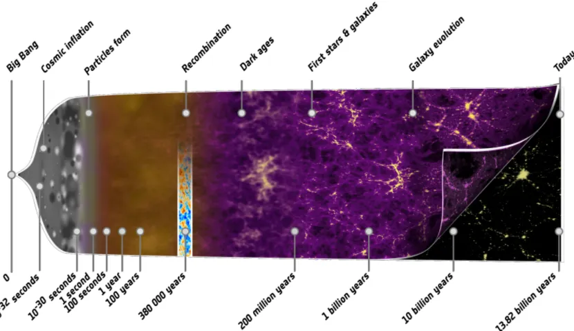
Figure 1.1: Annotated visualization of the cosmic timeline spanning the age of the universe, starting with the Big Bang and ending at present day. From left to right: a period of cosmic inflation (grey) results in the rapid expansion of the universe into a tightly-coupled photon-baryon plasma (brown). Photons decouple from the plasma during recombination, allowing baryons and dark matter to gravitationally collapse into large-scale structure (purple/black). See text for additional details. Figure courtesy of ESA - C. Carreau.

tational collapse because of their Coulomb interaction with these photon-coupled electrons,

but this was not the case for all massive particles: an exotic form of matter known as cold

dark matter (CDM)2_{, which only couples to other particles via gravity, is thought to have}

contributed to the growth of inflationary gravitational fluctuations throughout this period.

As the plasma temperature dropped below the ionization threshold, the free-electron

frac-tion began to decline rapidly as neutral hydrogen was formed, rendering Thomson scattering

ineffective. It was during this epoch of recombination that the universe became

transpar-ent, with photons streaming freely in all directions - the origin of the CMB radiation we

observe today. Once decoupled from photons, baryonic matter was free to interact with

the underlying dark matter density fluctuations, forming increasingly massive filamentary

structures as the universe continued to expand. This early era of unimpeded gravitational

2

(13)

collapse became known as the Dark Ages (due to the lack of significant sources of radiation)

and lasted until the local matter density became large enough to form the first stars and

galaxies - approximately 200 million years after the Big Bang. As increasingly larger and

more complex objects such as galaxy clusters began to coalesce and evolve over the next

few billion years, large scale structure started to take on the familiar hierarchical framework

we observe today. While the universe continued to steadily evolve in this manner through

present times, its expansion began to accelerate over the past 4 billion years - a phenomenon

that has been attributed to the presence of a mysterious dark energy. Figure 1.1 provides a

useful visualization of the cosmic timeline described above, highlighting many of the

impor-tant epochs and events. Since numerous observable properties of the CMB depend critically

on the physics that drive these events, a closer examination is certainly warranted.

1.1.1 Foundations

Before diving into the various physical phenomena of interest, we must first consider the

dynamical foundations of the universe in which they take place. Let us begin by invoking

the cosmological principle, which posits that the universe is both spatially homogeneous

and isotropic at sufficiently large scales3_{. Since the latter is supported by a variety of}

observational evidence (including the CMB), and the former holds true for our observable

universe and has yet to be otherwise falsified, this seems like a good starting point. Following

Carroll [22], let us explore the behavior of such a universe by introducing its metric:

ds2 =₋dt2+a2(t)

dr2

1₋κr2 +r 2_d_Ω2

(1.1)

wherea(t) is a time-dependent scale factor,ris the radial coordinate, dΩ2 ₌_dθ2_{+ sin}2_{θ dφ}

is the spherical surface metric, κ is a curvature parameter, and we have set c = 1. This

is known as the Friedmann-Robertson-Walker (FRW) metric, and describes a maximally

spatially symmetric universe that is either negatively curved (κ < 0), positively curved

(κ >0), or completely flat (κ= 0). Since the dynamics are ultimately governed by general

3

(14)

relativity, we will use this metric to find solutions to Einstein’s equation:

Gµν ≡Rµν−

1

2Rgµν = 8πGTµν (1.2)

where Gµν is the Einstein tensor, Rµν is the Ricci tensor (and R ≡ Rµµ its trace), gµν is

the metric tensor, Tµν is the energy-momentum tensor, and G is Newton’s gravitational

constant. This may also be written in the following, slightly more convenient form:

Rµν = 8πG

Tµν−

1 2T gµν

(1.3)

whereT =Tµ

µ is the trace of energy-momentum tensor.

Since Rµν depends only on the metric, we do not need any additional information to

evaluate the left-hand side of Equation 1.3. For the FRW metric given in Equation 1.1, the

Ricci tensor is diagonal, with the only non-zero components being:

R00=₋3a¨ ˙

a

R11=

a¨a+ 2 ˙a2_{+ 2}_κ

1−κr2

R22=r2 a¨a+ 2 ˙a2+ 2κ

sin2θ (1.4)

where ˙a and ¨aare the first and second derivatives of the scale factor with respect to time.

That leaves the right-hand side of Equation 1.3, for which we need to define Tµν. Since

we have already assumed isotropy and homogeneity in choosing the metric, let us extend

these assumptions to the mass and energy constituents of the universe by modeling them as

a perfect fluid at rest (in co-moving coordinates) with time-dependent energy density ρ(t)

and isotropic pressurep(t). The energy-momentum tensor for such a fluid is given by:

(15)

where we have chosen to write the tensor with one raised index for the sake of convenience.

This allows us to re-write Equation 1.3 as follows:

Rµν = 8πG

gµαTαν−

1

2(3p−ρ)gµν

(1.6)

Since both sides of the above are diagonal, we are left with four separate equations. As a

consequence of isotropy, however, only two of these are actually independent:

H2₌ 8πG

3 ρ−

κ

a2 (1.7)

¨

a a =−

4πG

3 (ρ+ 3p) (1.8)

where we have introduced the Hubble parameter H _≡ dln(_dta) = a˙

a - a measure of the

logarithmic expansion rate. Equations 1.7 and 1.8 are collectively known as the Friedmann

equations; taken together, they dynamically relate the geometry (expansion and curvature)

of the universe to the energy density and pressure of its constituents.

To gain a more detailed understanding, it is helpful to write the first Friedmann equation

in terms of a parameter called the critical density, which is defined as:

ρc=

3H2

8πG (1.9)

With this change of variables, Equation 1.7 becomes:

ρc=ρ−

3κ

8πGa2 (1.10)

The above equation provides a useful relation between curvature and energy density in an

FRW universe: if the total energy density is equal to the critical density, κ must be zero

- the universe is flat. If, on the other hand, the total energy density is not equal to the

critical density, the universe must have non-zero curvature (positive if it is less than, and

(16)

compact form by writing it in terms of the density parameter Ω _≡ ρ/ρc, which measures

the ratio of total energy density to the critical density:

1 = Ω + Ωκ (1.11)

where we have defined Ωκ=−_H2κ_a2 as the curvature “density” parameter4. Since the total energy density of the universe is a sum of its constituent species, we may likewise expand

Ω as a sum of the individual density parameters:

Ω = Ωm+ Ωr+ ΩΛ (1.12)

where the subscripts m,r, and Λ refer to matter, radiation, and dark energy, respectively.

Recent observations of the CMB have shown the present-day universe to be spatially flat

(Ωκ,0 <0.005) with a matter density parameter of Ωm,0= 0.3089±0.0062 and a negligible

contribution from radiation [89]. According to Equations 1.11 and 1.12, this implies that

the majority of the energy density in the universe today (_∼ 70%) is in the form of dark

energy - a conclusion which is supported by measurements of other cosmological probes [62].

But what exactly is dark energy, and why does it dominate the universe today? Though

there are numerous theories and explanations, one of the most common (and also simplest)

models is that of a cosmological constant Λ in Einstein’s equation:

Gµν+ Λgµν = 8πGTµν (1.13)

This results is an additional energy density term in the first Friedman equation (1.7):

ρΛ=

Λ

8πG (1.14)

Since Λ is (by definition) a constant, the dark energy density remains static as the universe

evolves with the scale factor. This is not, in general, true for the other components that

4

(17)

contribute to the total energy density. To understand why, let us examine the conservation

of the energy-momentum tensorTµ

ν, which is defined in Equation 1.5:

0 =∇µTµν =∇µTµαgαν (1.15)

where _∇µ is the covariant derivative. The ν = 0 component of the above equation yields

the following useful relation between the energy densityρ and the scale factora:

0 =_∇µTµ0g0ν =∇µTµ0= ˙ρ+ 3

˙

a

a(ρ+p) (1.16)

Because we are only considering perfect fluids, the pressure will depend linearly on the

energy density, yielding the following equation of state:

p=wρ (1.17)

where w is a constant. We may thus eliminate the pressure dependence in Equation 1.16

and are left with a simple first order differential equation inρ:

˙

ρ

ρ =−3(1 +w)

˙

a

a (1.18)

Integrating Equation 1.18 and setting the present day scale factor to one (a0 = 1), we obtain

a powerful expression for the evolution of the energy density:

ρ=ρ0a−3(1+w) (1.19)

Based on Equations 1.14 and 1.19, it is obvious that we must have wΛ =−1 for dark

energy described by a cosmological constant (which is why it is often referred to a as a

fluid with negative pressure). The energy density of matter, on the other hand, scales

with the particle density and thus inversely with volume; since volume in an FRW universe

(18)

radiation, ρ also scales with (relativistic) particle density, but the evolution of the particle

(e.g. photon) energies themselves must now be taken into account. The wavelength5 _λ _of

relativistic particles grows with the scale factor just like any other linear spatial separation,

effectively resulting in a redshift. For particles emitted in the past (scale factor a) and

observed today (a0 = 1), this cosmological redshiftz is defined as:

a= 1

1 +z (1.20)

Since the individual energy of these particles scales as λ−1_{, the overall energy density of}

radiation must therefore scale asρr=ρr,0a−4 with an equation of statewr= 1/3. Inserting

these scaling relations into Equation 1.7 while making a few other substitutions, we obtain

a dynamical model for the evolution of the universe in terms of the present-day values of

some important cosmological parameters:

H(z)2=H₀2

Ωr,0(1 +z)4+ Ωm,0(1 +z)3+ Ωκ,0(1 +z)2+ ΩΛ,0

(1.21)

where ΩΛ,0 = ₃_HΛ2 0

is the present-day dark energy density parameter andH0≈70 km/s/Mpc

is the Hubble constant - the current value of the Hubble parameter. From Equations 1.19

and 1.21, we see that dark energy has not always been as important a factor as it is today;

both radiation (z&3000) and matter (3000&z &0.5) have, in different epochs, played a

dominant role in the expansion history of the universe.

1.1.2 Inflation

The cosmological dynamics that we introduced in the previous section do quite well at

explaining the evolution of the universe into its present-day form. There are, however,

a number of different fine-tuning problems that emerge when reconciling our observations

with the initial conditions, two of which are particularly severe: the horizon and the flatness

problem. The latter, as the name suggests, is based on the very low value of spatial curvature

5

(19)

measured in the universe today. To better understand why this might be a concern, recall

the curvature “density” parameter introduced in Equation 1.11:

Ωκ(z) =−

κ

H2₍_z₎(1 +z)

2 _(1.22)

whereH2₍_z_{) is given by Equation 1.21 and we have substituted the redshift}_z_{for the scale}

factor a(Equation 1.20). To get a sense of how Ωκ evolves, let us differentiate the above

expression with respect to redshift:

dΩκ

dz =−2 Ω 2

κ(z)

H2 0 κ

Ωr,0(1 +z) +

Ωm,0

2 −

ΩΛ,0

(1 +z)3

(1.23)

Note that - with the exception of fairly low redshifts (z . 0.7) - the quantity inside the

brackets will always be positive, meaning that the sign of dΩκ

dz will match that of Ωκ. Hence,

if Ωκ is positive, it will continue to increase; likewise, if it is negative, it will continue to

decrease. A flat universe is thus an unstable equilibrium throughout much of cosmic history,

with even the slightest curvature quickly growing larger during the radiation and matter

dominated eras; in early times, _|Ωκ| would had to have been many orders of magnitude

smaller than it is today. Why should the universe have been so precisely flat in the past?

The horizon problem arises from the finite age of the universe and the associated

limita-tions on causality. Let us examine the largest comoving distance over which particles could

have conceivably communicated with each other since the big bang by considering the path

of a photon. In a flat universe6_{, the total comoving distance that photons traveling along}

null geodesics will traverse sincet= 0 is given by the particle horizon:

dp=

Z t

0 dt0 a(t0₎ =

Z a

0

dln(a0)

a0_H (1.24)

Any two points separated by comoving distances greater than dp would thus have never

had the chance to be in causal contact with each other. Up to the epoch of recombination

6

(20)

and the release of the CMB, the universe had been either matter or radiation dominated;

the particle horizon at that time may therefore be computed by substituting Equation 1.21

into Equation 1.24 and neglecting the dark energy (and curvature) term:

dp(acmb) =H0−1

Z acmb

0

da0

p

Ωr,0+ Ωm,0a0

= 2H

−1 0

Ωm,0

p

Ωr,0+ Ωm,0acmb−

p Ωr,0

(1.25)

The comoving distance between an observer on Earth and a point on the surface of last

scattering for CMB photons may likewise be computed, though for simplicity we will neglect

dark energy and assume a matter dominated universe7_:

∆r=H₀−1

Z 1

acmb

da0

p

Ωm,0acmb

≈2H₀−1 (1.26)

Compared to ∆r, the particle horizon of the CMB is quite a bit smaller (more than an

order of magnitude); since two parts of the universe from which the CMB originated may

be separated by up to 2∆r (i.e those in opposing directions on the sky), there must have

been a large number of patches on the surface of last scattering that could not have been

in causal contact with one another. So how is it possible that the CMB we observe is so

homogeneous across the entire sky? Or, put another way, why should we expect causally

disconnected parts of the universe to end up in such a precisely homogeneous state?

A solution to both the horizon and the flatness problem is provided by a period of

rapid exponential expansion, or inflation, in the very early universe. Since an exponentially

expanding scale factor requires that the Hubble parameter be roughly constant, the integral

on the right hand side of Equation 1.24 will diverge at low values of a. Hence, there is no

particle horizon during inflation: all scales must have been in causal contact at very early

times. A constant Hubble parameter also drives down curvature: since Ωκ ∝(aH)−2, an

exponentially increasing scale factor results in a rapidly flattening universe. While there

7

(21)

φ V(φ)

φstart φend

Inflation

Reheating

log(t) log(a)

a_∝eHt

Inflation

a∝

√_t

Radiation

Figure 1.2: Left: A qualitative sketch of scalar field inflation. A scalar fieldφdrives inflation by starting to slowly roll down a potential V(φ) at φstart until its kinetic energy becomes

too large atφend. At that point, inflation is no longer sustainable and a period of reheating takes place as φdecays into other energetic particles while oscillating at the bottom of the potential. Right: The evolution of the scale-factor: during inflation, the growth of a is exponential, but then converges to the expansion rate of a radiation dominated universe.

are many differing theories and models that describe the underlying physics of inflation,

one of the most simple is that of a homogeneous scalar fieldφin a potentialV(φ) [14]. The

equations of motion for such a field evolving in a flat gravitational background are given by:

¨

φ+ 3Hφ˙+V0 = 0 (1.27)

H2 = 3 8πG

1 2φ˙

2₊_V

(1.28)

where a prime denotes a derivative with respect toφ. Since the Hubble parameter must be

approximately constant during inflation to guarantee exponential expansion, the quantity

enclosed by brackets on the right-hand side of Equation 1.27 should not vary much with time.

One way to achieve this is to impose a “slow-roll” condition, where φslowly “rolls down”

the potential V over a period of time which is sufficiently long to sustain the inflationary

expansion. This condition may be expressed quantitatively as:

˙

φ2 V and _|φ¨_{| |}3Hφ˙_|,_|V0_| (1.29)

(22)

that such a state is maintained. These requirements may also be expressed in terms of the

potential by defining the two slow-roll parameters εφ and ηφ:

εφ= 4πG

V0

V

2

(1.30)

ηφ= 8πG

V00

V (1.31)

where εφ,|ηφ| 1 throughout the inflationary epoch. As φ finally gains enough kinetic

energy such that 1 2φ

2_≈_V_{, the slow-roll parameters grow to order unity and inflation comes}

to an end. What follows is a transition to radiation domination: asφoscillates at the bottom

of the potential and decays into a series of energetic particles, the universe begins to reheat

from the highly overcooled state that resulted from exponential expansion. This evolution

of the scalar field, along with the behavior of the scale factor, is shown in Figure 1.2.

So far, our description of inflation has been a macroscopic one, with φbehaving like a

classical field within its potential. But this does not provide a complete picture: we must

also account for possible quantum fluctuations of the field:

φ(t,x) = ¯φ(t) +δφ(t,x) (1.32)

where ¯φ(t) is the underlying homogeneous field (described above). Since these fluctuations

affect the local evolution of the scale factor, they have the ability to induce both scalar and

tensor perturbations in the metric (the latter of which corresponds to propagating

gravita-tional waves). A powerful prediction of inflation is that the fluctuation power spectrum be

nearly scale invariant; this may be understood by considering the amplitude of an individual

Fourier mode, which initially scales with its wavenumberk. As the universe exponentially

expands during inflation, k will shrink proportional to a−1_{, resulting in a rapid decrease}

in the amplitude. Once the wavelength (∼k−1_{) expands beyond the Hubble horizon} _H−1_,

however, the mode can no longer evolve and the amplitude is frozen out at ∼ k/a = H.

(23)

mode will freeze out at nearly the same amplitude. The resulting dimensionless spectrum

is thus very close to scale invariant, depending only onH (or equivalentlyV):

Pφ(k) = 8πG

H2

4π2

k=aH

≈ (8πG)

2

3

V

4π2

k=aH

(1.33)

where the vertical bar indicates that either H orV should be evaluated when a particular

mode exits the horizon (k = aH). The corresponding spectra of scalar (PR) and tensor

(Pt) fluctuations in the metric are then given by:

PR(k) =

8πG

8π2 H2 εφ

k=aH

≈ (8πG)

2

24π2 V εφ

k=aH

(1.34)

Pt(k) =

2(8πG)

π2 H 2

k=aH

≈ 2(8πG)

2

3π2 V

k=aH

(1.35)

where we have chosen to define the scalar fluctuations in terms of invariant comoving

cur-vature perturbations R, which include both gravitational and density perturbations:

R=ψ ₋ 1

3

δρ

¯

ρ+ ¯p (1.36)

For convenience, these spectra are often parameterized by wavenumber k and their

corre-sponding spectral indices ns and nt, such that:

PR(k) =AR(k0)

k k0

ns−1

(1.37)

Pt(k) =At(k0)

k k0

nt

(1.38)

where k0 is an arbitrary pivot scale. Note that for slow-roll scalar field inflation, it can be

shown that the spectral indices are directly related to the slow-parameters εφand ηφ:

ns= 1 + 2ηφ−6εφ (1.39)

(24)

Although other models of inflation differ in their particular formulation and

parameter-ization of both ns and nt, they all predict some degree of deviation from perfect scale

invariance. This effect has actually been observed in the scalar perturbation spectrum,

with recent measurments revealing a slighly negative tilt (ns= 0.9667±0.0040) [89].

1.1.3 Primordial Plasma

Following inflation and the subsequent period of reheating, the universe still remained in an

incredibly dense and energetic state (especially when compared to modern times).

Temper-atures in excess of 1015_{K inhibited the formation of all but the most elementary of particles}

(e.g. quarks, electrons, neutrinos, and photons) while ensuring that those which did form

remained highly relativistic - this marked the beginning of the radiation dominated era. As

the universe expanded and the temperature dropped, heavier particles began to decay or

were annihilated in matter-antimatter collisions, while lighter particles were held in

con-stant thermal equilibrium with the radiative environment. At temperatures below 1012 _K,

strong interactions between the remaining quark species became powerful enough to bind

them, leading to the formation of protons and neutrons - the first baryons in the universe.

Weak interactions, on the other hand, lost their effectiveness at lower temperatures; below

1010 _{K, particles such as neutrinos and neutrons, which had originally been held in thermal}

equilibrium by these interactions, began to decouple from the primordial plasma. Since

neutrinos interact primarily via the weak force (and to a lesser extent, gravity), they were

no longer bound to other particles after decoupling and began free-streaming in the form

of a cosmic neutrino background (CNB). The CNB constitutes a significant fraction of the

total radiative energy density in the universe while the neutrinos remain relativistic, with

a density parameter comparable to that of photons [2]:

Ων =Neff

7 8

4 11

4/3

Ωγ (1.41)

where Ωγ is the photon density parameter and Neff is the effective number of neutrino

(25)

interac-tions with protons, eventually become bound in atomic nuclei when the temperature drops

below 109 _{K during the epoch of Big Bang nucleosynthesis (BBN). While BBN is}

respon-sible for the primordial abundances of a variety of light elements and their isotopes (e.g.

deuterium, tritium, helium-3, lithium and beryllium), the overwhelming majority of

neu-trons are captured in the form of Helium-4. The primordial helium abundance thus serves

as an important indicator for the nuclear evolution of the early universe.

At the end of the BBN era, the primordial plasma was predominantly composed of

photons, free electrons, and atomic nuclei, all of which interacted via frequent Coulomb,

Compton, and Thomson scattering events. The result was a tightly-coupled photon-baryon8

fluid whose dynamics were governed by gravity, internal pressures, and a characteristic speed

of sound that depended on the relative energy densities of the constituent species [50]:

cs=

1 p

3(1 +R) (1.42)

where R _≡ 3₄ρb

ργ is the baryon-photon density ratio. Since cosmic inflation had induced

small scale-invariant perturbations in the energy density and gravitational potential, this

fluid did not exist in a state of spatial equilibrium: on scales equal to the contemporaneous

sound horizon s =R

csdη (where η is the conformal time variable), photons and baryons

began falling into nearby gravitational potential wells. As the fluid began to compress at the

bottom of the potential, increasing photon radiation pressure drove it back apart, inducing

an oscillatory pattern in the local energy density; during radiation domination (R 1) and

absent any damping or other secondary effects, these acoustic oscillations are given by:

δρ(η) =δρ,0cos(ks)≈δρ,0cos

kη

√

3

(1.43)

whereδρ=δρ/ρis the relative density perturbation. As the universe grows older, the sound

horizon expands, allowing additional modes to begin oscillating at larger scales. Modes well

outside the sound horizon (kη1), however, remain frozen at their initial amplitudes.

8

(26)

1.1.4 Recombination

The photon-baryon plasma remained tightly coupled while electron-photon scattering

inter-actions were able to maintain kinetic equilibrium. As the universe cooled with its expansion,

however, the efficiency of these interactions began to decline; consider the Thomson

scat-tering rate Γ of a photon as a function of the scale factora[31]:

Γ =Xe

σT

mp

ρm,0a−3 (1.44)

where Xe is the free electron fraction, ρm,0 is the matter energy density today, mp is the

proton rest mass, σT is the Thomson scattering cross section, and the effects of helium

nuclei have been neglected9_{. When this rate falls below the Hubble time} _H−1_{, scattering}

becomes inefficient and photons begin to decouple from their baryonic counterparts. Since

the universe was either radiation or matter dominated throughout much of its history, the

Hubble parameter scales by at mostH∝a2 _{(see Equation 1.21), making decoupling}

practi-cally inevitable. Nevertheless, the actual timing and duration of this process were governed

by the dynamics of another important event: the “recombination”10 _{of electrons and}

pro-tons to form neutral hydrogen nearly 380,000 years after the Big Bang. The free electron

fraction in the plasma may be reasonably approximated using the Saha ionization equation:

X2

e

1₋Xe

= 1

ne+nH

"

meT

2π

3/2

e−(me+mp−mH)/T

#

(1.45)

where ne and nH are the electron and hydrogen number densities, and me, mp, and mH

are the electron, proton, and hydrogen rest masses. Since the mass of hydrogen is less the

sum of the individual proton and electron masses, Equation 1.45 predicts a steep decline

inXe as the temperature drops below a critical threshold. This is precisely what occurred

during the epoch of recombination, resulting in a relatively rapid decoupling of photons as

the scattering rate fell well below H−1 _{- this is the radiation we now observe as the CMB.}

9_{This does not significantly alter the qualitative description of the scattering process.}

10

(27)

1.2 Models and Measurements

The field of modern cosmology has come a long way since the day Penzias and Wilson

first made their pivotal discovery. Thanks to a plethora of highly sensitive measurements,

computer assisted modeling, and theoretical insights, we now have a robust understanding

of both the spatial and spectral properties of the CMB, and how these relate to some

of the most important events in the early universe. The radiation is well described by a

blackbody spectrum, has a nearly uniform temperature across the entire sky, and is almost

completely unpolarized. Tiny anisotropies in both temperature and polarization break this

perfect mold, but also allow us to test a large variety of cosmological models with increasing

precision. Combined with data from the infrared, visible, and X-ray part of the spectrum,

the CMB has become an invaluable asset to exploring the fundamental physics of the cosmos.

1.2.1 Spectral Properties

It is easy to think of the origin of CMB photons as the surface of last scattering during

recombination, but this is merely what its name suggests: a point in time at which these

photons last scattered. Their true origin may actually be traced back to the early days of

the primordial plasma at a redshift of z& 2_×106_{, when photon emission and absorption}

via radiative Compton scattering was highly efficient [58]. At that point, the plasma was in

complete thermal equilibrium, with a blackbody radiation temperature in excess of 106 _K.

Since the universe expanded adiabatically into its present state, we should expect the CMB

to retain this blackbody spectrum, albeit at a much lower temperature. This is indeed

the case: detailed spectral measurements made by the FIRAS instrument on the Cosmic

Background Explorer (COBE) satellite have shown the CMB to be a near perfect blackbody

(rms deviations _O(10−5_{)), with a temperature of} _T

CMB = 2.725±0.001 K [37, 38]. The

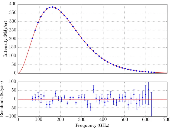
measured spectrum and blackbody residuals are shown in Figure 1.3.

As the universe expanded and the primordial plasma cooled, radiative Compton

(28)

Figure 1.3: The CMB blackbody spectrum measured by the FIRAS instrument on the COBE satellite. The plot at the top shows the measured spectrum (blue) and the curve for a theoretical blackbody spectrum with temperature T = 2.725 K (red). The plot on the bottom shows the residuals between the data and the blackbody curve - note the differing scales on the y-axes. Data based on measurements provided in Table 4 of Fixsen et al. [38].

and dissipation could no longer be completely thermalized and now had the potential to

induce distortions in the CMB blackbody spectrum. At relatively high redshifts (z&105_),

traditional Compton scattering was still effective at preserving kinetic equilibrium [23],

implying that any distortions produced at that time must conform to a Bose-Einstein

dis-tribution. The modified spectrum is then given by:

Iµ(ν) =

2hν3 c2

1

ekB Thν +µ₋₁

(1.46)

where T is the photon temperature and µ is a frequency-dependent chemical potential

which vanishes in the limit of complete thermal equilibrium. Consequently, these

high-redshift distortions are known as “µ-type” distortions; they may arise from phenomena

(29)

scattering also becomes inefficient, bringing an end to kinetic equilibrium in the plasma and

allowing more complex “y-type” distortions to be produced. One of the most significant

of these is the thermal Sunyaev-Zel’dovich (tSZ) effect, whereby low-energy photons are

boosted to higher frequencies by inverse Compton scattering off energetic electrons. The

resulting spectral distortion ∆ItSZ is given by [108]:

∆ItSZ(ν) =y xex

ex₋₁

xe

x_{+ 1}

ex₋₁ −4

I0(ν) (1.47)

where x = _khν

BT, I0 is the original spectrum, and the Compton y-parameter y - which

measures the strength of the distortion - is defined as:

y= σT

mec2

Z

nekBTedl (1.48)

wherene,Te, andmeare the electron number density, temperature, and mass, respectively,

σT is the Thomson cross section, and the integral is evaluated along the path of the radiation.

While measurements by FIRAS have limited the total magnitude of diffuse µ and y-type

distortions to be less than 9_×10−5 _{and 15}_×₁₀−6_{, respectively, localized values of}_{y >}₁₀−4

have been measured for the tSZ effect in the presence of massive galaxy clusters [76].

1.2.2 Temperature Anisotropies

One of the most elementary yet consequential properties of the CMB is how remarkably

isotropic it is11_{- every direction one looks on the sky, its temperature is incredibly uniform.}

Much of this radiation’s scientific potential, however, is not found in its isotropy, but in

the many small, yet interesting departures from it. The largest of these anisotropies takes

the form of a simple dipole pattern on the sky, whose origin is the relativistic Doppler shift

induced by the relative motion of the Earth with respect to the CMB rest frame:

∆T

T =βcosθ (1.49)

11

(30)

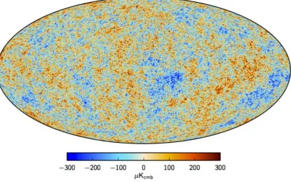
Figure 1.4: Post-processed full-sky map of the primary CMB temperature anisotropies in galactic coordinates as measured by the Planck satellite and presented in Planck Collabo-ration et al. 2016a [87]. These fluctuations are a reflection of the density and gravitational potential perturbations at the time of photon decoupling over 13.4 billion years ago.

where β is our relative velocity with respect to the CMB (expressed as a fraction of the

speed of light), and θ is the angular displacement on the sky with respect to the velocity

vector. The magnitude of this effect is of order 10−3 _{K - only a small fraction of the}

CMB blackbody temperature, but still orders of magnitude greater than any other observed

fluctuations. In 1992, the DMR instrument on the COBE satellite was the first to detect

the intrinsic temperature anisotropies of the CMB on large angular scales (_∼ 10◦_{) at an}

amplitude of order 10−5 _{K [107]; a more recent, higher resolution measurement made by}

the Planck satellite [87] is shown in Figure 1.4. The origin of these tiny temperature

fluctuations may be traced back to the last scattering of CMB photons during the epoch

of recombination (§1.1.4): spatial inhomogeneities in the energy density resulting from the

(31)

induce local variations in the temperature of the plasma. These differences are then reflected

in the temperature-shifted spectra of free-streaming CMB photons after decoupling.

The fluctuations we observe today are actually not a perfect image of those found on

the surface of last scattering; the transfer function between the two, which incorporates a

number of additional physical effects, is given by the Sachs-Wolfe equation [66]:

Θ_|obs = (Θ0+ψ)|dec+ ˆn·vb|dec+

Z η0

ηdec

φ0+ψ0

dη (1.50)

where Θ ≡ ∆T

T is the temperature fluctuation in a given direction ˆn, ψ and φ are the

gravitational potential and spatial distortion, respectively, vb is the bulk velocity of the

photon-baryon fluid, and η is the conformal time variable. The subscripts ’dec’ and ’0’

refer to the time of decoupling and today, and primes indicate derivatives with respect to

conformal time. The first term on the right-hand side of Equation 1.50 is known as the

Sachs-Wolfe effect and captures the interaction of photons with their local gravitational

environment: photons scattering from over-dense regions experience a red-shift as they

climb out of gravitational potential wells, while those from under-dense regions experience a

corresponding blue-shift. This results in warmer regions appearing slightly cooler and colder

regions slightly warmer than they otherwise would; on large scales, where gravitational

potentials did not have the opportunity to decay prior to decoupling, this effect is strong

enough to invert the temperature fluctuations. The second term in Equation 1.50 is simply

the Doppler shift produced by bulk motions in the photon-baryon fluid at the time of

decoupling; it is most pronounced on scales at which acoustic oscillations are transitioning

between minima and maxima (i.e the bulk velocity is highest). The third term, which is

known as the integrated Sachs-Wolfe effect (ISW), describes the impact of time-varying

gravitational potentials and spatial distortions on the photon temperature spectrum. If,

for example, a photon traverses a decaying potential well, it will experience a net increase

in energy since the initial blue-shift during infall will be larger in magnitude than the

subsequent redshift (when the potential is weaker). Slowly varying gravitational potentials

(32)

1.2.3 Angular Power Spectrum

Maps such as the one shown in Figure 1.4 are not only visually striking, but also contain

a wealth of information about the various physical processes responsible for producing the

CMB temperature fluctuations (including those described in in the previous section). A

powerful method for extracting this information is to examine the statistical properties of

the fluctuations by computing their two-point correlation function in angular space. Since

we observe the CMB on the surface of a sphere, it is natural to expand its temperature field

on the sky in a geometrically appropriate basis of spherical harmonicsY`m:

Θ(ˆn) =

∞

X

`=1

`

X

m=−`

a`mY`m(ˆn) (1.51)

where ˆnis a given direction on the sky,`andmare the multipole moment and azimuthal de-gree of freedom of the spherical harmonics, respectively, and we have ignored the monopole

term`= 0 (i.e. the average temperature). The complex coefficientsa`m, which specify the

amplitude and phase of each harmonic mode, are given by:

a`m =

Z

d3_k

2π2 (−i)

`_Y

`m(ˆk) Θ`(k) (1.52)

where Θ`are the Fourier-space multipole moments of the temperature fluctuations Θ. Since

these coefficients describe a Gaussian random field, the expectation value for any particular

a`m must vanish; all their statistical information is thus contained within the two-point

correlation function, which may be written as:

ha`ma∗`0_m0i=δ_``0δ_mm0C_` =δ_``0δ_mm0 1 2π2

Z _dk k

Θ`(k)

R(k)

2

PR(k)

!

(1.53)

where R and PR are the scalar curvature perturbations and their dimensionless power

spectrum, respectively, as defined in §1.1.2. The quantitiesC`, which are expanded inside

the brackets in the above equation, are known as the angular power spectrum - they encode

(33)

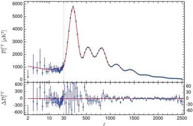
Figure 1.5: Angular power spectrum of the CMB temperature fluctuations as measured by the Planck satellite and presented in Planck Collaboration et al. 2016b [92]. The spectrum is plotted as the power per logarithmic interval_D`=`(`+1)C`/(2π). The red curve represents

the best-fit cosmological model for the data, with the corresponding residuals plotted in the bottom panel. Note the difference in the data at high and low multipoles, as indicated by the dotted line at`= 30. This is due to the use of different spectral estimation algorithms.

observe today. While a highly precise measurement of this spectrum over a broad range

of angular scales12 _{would be a valuable asset to modern cosmology, there is a fundamental}

statistical limitation on the uncertainty which increases significantly at large angular scales

(small `). Consider the best estimator ˆC` for the true angular power spectrumC` given a

measured set of spherical harmonic expansion coefficients ˜a`m:

ˆ

C`=

1 2`+ 1

`

X

m=−`

|a˜`m|2 (1.54)

where we were able to take the average over all values of m due to the statistical isotropy

of the temperature fluctuations (and thus the spectrum). Since the number of available

12

(34)

azimuthal degrees of freedom decreases at lower values of`, we should expect the statistical

uncertainty of the estimation to increase; this is indeed the case, with the variance of the

estimator defined in Equation 1.54 scaling as:

h( ˆC`−C`)2i=

2 2`+ 1C

2

` (1.55)

This “cosmic variance”, as it is more commonly known, is a reflection of the fact that we

can only measure a single realization of the universe from our fixed location here on Earth.

The CMB temperature angular power spectrum - or TT spectrum - measured by the

Planck satellite is shown in Figure 1.5; it contains a number of interesting features that are

directly related to some of the physics discussed earlier in this chapter. The most prominent

of these is a series of harmonic peaks that start oscillating near a multipole of`_∼200, and

then continue with decreasing amplitude down to smaller angular scales. These peaks are

the result of the acoustic oscillations in the photon-baryon fluid (_§1.1.3): the first peak

represents modes that have undergone a single compression between the time they entered

the sound horizon and the time of photon decoupling, while the second represents those

that have undergone both a compression and a rarefaction in the same time interval. The

pattern continues at higher values of`, but with an increasingly damped amplitude due to

the scattering of photons between hot and cold regions of the plasma toward the end of

the decoupling epoch. The scale of the peaks is determined by the angular size the sound

horizon at decoupling, which depends on the expansion history of the universe and therefore

its curvature and the energy densities of its constituents. The peak amplitudes, on the other

hand, are specifically sensitive to the baryon density, since a higher baryon/photon ratio

enhances compression and reduces rarefaction. Note that the power spectrum does not

vanish between peaks - this is due to maxima of the Doppler effect (§1.2.2) at scales where

the fluid velocity is greatest. At relatively large angular scales (` < 30), the spectrum is

reasonably flat, forming what is known as the Sachs-Wolfe plateau. It consists of modes that

never entered the sound horizon prior to decoupling, and whose amplitude is determined by

(35)

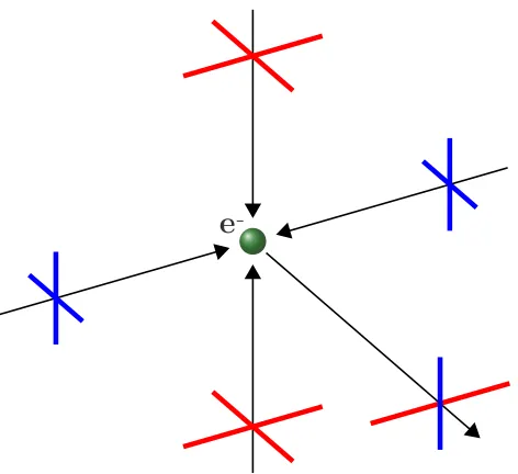
e

Figure 1.6: An electron surrounded by a quadrupole temperature anisotropy in its local radiation environment. Red and blue lines indicate polarization components from hotter and colder temperatures, respectively. During Thomson scattering, this pattern produces a net linear polarization which aligns with the cold axis of the quadrupole.

1.2.4 Polarization

Fluctuations in temperature are not the only anisotropies of great interest: in 2002, the

DASI experiment [61] made the first detection of the faint polarization signature of the CMB

at an amplitude of order 10−6_{K, opening the door to a whole new era of precision cosmology.}

Unlike the intrinsic temperature fluctuations, polarization of the CMB is mostly a scattering

phenomenon, requiring a quadrupole anisotropy in the local radiation environment in order

to be produced. This situation is shown schematically in Figure 1.6: since only those

polarization components perpendicular to the final propagation direction are effectively

Thomson scattered, a temperature quadrupole will generate a net linear polarization parallel

to its cold axis. While the photon-baryon fluid was tightly coupled prior to recombination,

the local temperature was well-equilibrated and any anisotropy would have been rapidly

destroyed. Polarization of the CMB would thus have only been possible during the epoch

of decoupling, a time when photon diffusion was taking place and the Thomson scattering

(36)

Figure 1.7: E and B-mode polarization patterns illustrated in terms of the coordinate-referenced Stokes parameters Q and U. The E-mode patterns exhibit even parity while those of the B-mode exhibit odd-parity. The reference coordinate system for Q and U is shown in the center. Figure courtesy of Sigurd Naess.

Polarized signals are typically expressed in terms of the Stokes parameters - a

coordi-nate dependent basis that decomposes the electric field of the radiation into an intensity

componentI, two linear polarization componentsQandU, as well as a circular polarization

component V. Since there is no mechanism by which circular polarization is generated in

the CMB, we ignore V and express the remaining parameters in terms of the orthogonal

components of the electric field vectorE in thex-ycoordinate system defined in Figure 1.7:

I =_|Ex|2+|Ey|2 (1.56)

Q=_|Ex|2− |Ey|2 (1.57)

(37)

Although these parameters can fully describe the CMB polarization fluctuations, they still

require a reference coordinate system to be defined. Ultimately, we would like to characterize

the polarization components in the same manner as the temperature by measuring their

angular power spectra. Since Q and U are not rotationally invariant, they can not be

expanded in terms of spherical harmonics. Thus, let us define two different orthogonal

polarization fieldsE and B that do not depend on a choice of coordinates and satisfy:

E(ˆn) =

∞

X

`=1

`

X

m=−`

aE_`mY`m (1.59)

B(ˆn) =

∞

X

`=1

`

X

m=−`

aB_`mY`m (1.60)

whereaE

`m andaB`m are complex spectral coefficients. The E-mode and B-mode polarization

patterns are shown in Figure 1.7. E-mode patterns are either tangential or radial and

exhibit even parity, while the B-mode patterns resemble spirals and exhibit odd parity.

CMB polarization produced by a scalar temperature perturbation quadrupole will always be

in the form of E-modes, while that produced by the gravitational wave induced quadrupole

of tensor perturbations may be in either form. Gravitational lensing by large scale structure

between us and the surface of last scattering may also produce B-modes by breaking the

(38)

Chapter 2 The Atacama Cosmology Telescope

Sitting on top of a desert plateau in northern Chile, the Atacama Cosmology Telescope

(ACT) is one of the largest CMB observatories in the world. ACT was originally

commis-sioned back in 2006 for the Millimeter Bolometer Array Camera (MBAC), a multi-frequency

receiver designed to measure the CMB temperature anisotropies on small scales [111]. The

telescope itself stands 12 meters tall and is surrounded by a slightly taller (13 meter)

sta-tionary ground screen that serves to shield the receiver from spurious ground emission. The

movable portion of the structure weighs approximately 40 tons and contains the elevation

drive, the primary and secondary reflectors, an additional co-moving ground-screen, as well

as a temperature-controlled cabin that houses the receiver and all associated electronics

(see Figure 2.1). In 2013, ACT was retro-fitted to house the new ACTPol cryostat (see

§3) - while many of the telescope’s original components remained untouched, parts of the

receiver cabin had to be modified to accommodate the instrument’s larger footprint (∼1.5

m3_{). Additional adjustments also had to be made to the position of the secondary reflector}

in order to re-focus the optical system - these are described in §2.2.

2.1 Location

The ACT site is located at an elevation of 5,190 meters on a small plateau at the foot of

(39)

(40)

South) permits observations over more than 50% of the sky and allows for overlap with many

other millimeter and optical surveys near the celestial equator . One of the primary reasons

for choosing this location, however, is its exceptionally dry weather and limited atmosphere,

both of which are equally important to making high signal-to-noise measurements of a

cosmic signal at millimeter wavelengths. The Earth’s atmosphere not only absorbs part of

the incoming signal before it reaches the ground, but also emits radiation at a (typically)

much higher intensity in the same spectral band. This extra atmospheric emission increases

the in-band loading on the detectors, elevating noise levels and reducing the overall dynamic

range of the instrument.

2.1.1 Atmospheric Optical Depth

To understand the relationship between elevation, water content, and emission / absorption

in the atmosphere, one must examine total optical depth τ. This is because both

atmo-spheric transmittance _T and brightness temperature TB at a given frequencyν depend on

this quantity1_:

T(ν) =e−τ(ν)X (2.1)

TB(ν) =Tatm1₋e−τ(ν)X (2.2)

where Tatm is the effective temperature of the atmosphere and X is known as the airmass

- a dimensionless parameter that depends on one’s observing angle with respect to zenith.

Thus, larger optical depth results in both reduced signal transmittance and greater

atmo-spheric emission (i.e. brightness temperature). Given an atmosphere composed of multiple

constituent species (e.g. N2, O2, H2O) and neglecting the effects of scattering, we can define

τ as follows:

τ(ν) =X

i

τi(ν) =

X

i

Z ∞

z0

κi(ν)ρi(z0)dz0 (2.3)

1

(41)

Figure 2.2: Left: Optical depth at the ACT site for typical PWV values during the nominal observing season, simulated using the ALMA ATM model. Two oxygen absorption lines at 60 and 117 GHz as well as a water absorption line at 183 GHz are clearly visible. Also shown are the approximate locations of the ACTPol observing bands at 97 and 149 GHz. Right: Distribution of PWV values during ACTPol CMB observations from April 2015 through January 2016 - the median value during this period was 0.97 mm. The data was taken by a six-channel 183 GHz radiometer at the Atacama Pathfinder Experiment (APEX), approximately 8 km from the ACT site.

whereτi,κi, andρi(s0) are the optical depth, absorption coefficient, and elevation-dependent

density of species i, respectively, and z0 is the observer’s elevation. We immediately see

that optical depth increases as elevation decreases2 _{or the density of a constituent species}

increases. Furthermore, it is worth noting that the total water content in the atmospheric

column, typically referred to as precipitable water vapor (PWV), is simply the integral of

its density3_{. Thus, the optical depth due to water}_τ

w is directly proportional to PWV:

τw(ν) =κw(ν)

Z ∞

z0

ρw(z0)dz0=κw(ν)×PWV (2.4)

The Atacama Large Millimeter Array (ALMA), situated _∼ 10 km from the ACT site at

an elevation of 5040 meters, has developed sophisticated code for simulating atmospheric

optical depth based on Juan Pardo and Jos´e Chernicharo’s Atmospheric Transmission at

Microwaves (ATM) model [82]. The left side of Figure 2.2 shows the output of this model

2_{Making the realistic assumption that, on average, density does not increase with altitude.}

3

(42)

for various levels of PWV when configured for ACT’s elevation, as well as the approximate

locations of the ACTPol observing bands. The most significant contribution to the optical

depth comes from the H2O absorption line at 183 GHz, especially in the 149 GHz band

for higher values of PWV, although the O2 absorption lines at 60 and 117 GHz also play

a role. While the PWV range used to simulate optical depth is typical of ACT’s nominal

operating season from April through December (see the right side of Figure 2.2), average

values frequently exceed 3 mm during the remainder of the year, restricting observations.

However, it is important to note how these numbers compare to those at most other locations

around the world: on a “dry” winter day in Philadelphia (elevation = 12 meters, PWV =

8 mm), for example, the optical depth would reach 0.28 at 149 GHz - over ten times the

median value at the ACT site during a typical observing season.

2.1.2 Site Logistics

In addition to ALMA, numerous other millimeter observatories are located near the ACT

site. These include the Atacama Pathfinder Experiment (APEX), POLARBEAR, the

Cos-mology Large Angular Scale Surveyor (CLASS), and, until recently, the Atacama B-mode

Search (ABS). Despite the presence of these neighboring experiments, ACT’s location is still

considered remote by most standards. The nearest incorporated settlement, the town of

San Pedro de Atacama (population∼2000), is situated over 40 km away - about a one hour

drive on partially paved roads. San Pedro is also the location of ACT’s base station and

housing compound4_{, which serves as the telecommunications gateway to the outside world}

via a 10 Mbps internet link. Communications between the ACT site and the low elevation

base station are enabled by a two-way line-of-sight broadband microwave link operating at

5 GHz and a typical bandwidth of 100 Mbps, permitting large volume data transfers and

remote access to the telescope 24 hours a day.

Due to the site’s distance from the nearest inhabited areas, everything was designed

to be almost entirely self-contained. Electricity is generated on the premises by two 150

4_{Due to low oxygen levels at ACT’s high elevation site, visiting researchers are housed in a less harsh}

Exploring The Universe With The Atacama Cosmology Telescope: Polarization-Sensitive Measurements Of The Cosmic Microwave Background

University of Pennsylvania

ScholarlyCommons

Publicly Accessible Penn Dissertations

2017

Exploring The Universe With The Atacama

Cosmology Telescope: Polarization-Sensitive

Measurements Of The Cosmic Microwave

Background

Marius Lungu

Follow this and additional works at:

https://repository.upenn.edu/edissertations

Part of the

Astrophysics and Astronomy Commons

Recommended Citation

Exploring The Universe With The Atacama Cosmology Telescope:

Polarization-Sensitive Measurements Of The Cosmic Microwave

Background

TABLE OF CONTENTS

LIST OF TABLES

LIST OF FIGURES

Chapter 1

The Cosmic Microwave Background

1.1

Cosmic Evolution

1.2

Models and Measurements

e

Chapter 2

The Atacama Cosmology Telescope

2.1

Location