Obesity and Health-Care Costs in Switzerland: Dealing with Endogeneity in Non-Linear Regression Models

(1)

a Department of Business and Economics (WWZ), University of Basel, Peter Merian-Weg 6, P.O. Box, CH-4002 Basel, Switzerland. Email: stefan.meyer@unibas.ch.

Stefan Meyera

JEL-Classification: I11, I12, C26

Keywords: obesity, health expenditure, measurement errors, endogeneity, control functions

SUMMARY

(2)

1 BMI is defined as the individual’s body weight (kg) divided by the square of height (m2 ). 2 According to the Federal Statistical Office (FSO), this trend has been most pronounced among

men and elderly people. In 2012, for instance, 50.5 per cent of all Swiss men above the age of 15 were either overweight or obese, amounting to a BMI above 25 kg/m2 _{(FSO, 2012).} 3 In a follow-up study with 2006 data, Finkelstein et al. (2009) report even more pronounced

outcomes. Across all payers, obese people faced per capita spending that was up by 42 per cent (USD 1,429) compared to normal-weight individuals. In aggregate, the annual medical burden of obesity was found to be 9.1% of total medical spending.

1. Introduction

In Switzerland, the prevalence of obesity, defined as a body mass index (BMI) of at least 30 kg/m2, has increased significantly over the last decades.1 Between 1992 and 2012, the number of obese adults in Switzerland has more than dou-bled, reaching 10.3% of the total population in 2012. Over the same period, the share of people who were classified as overweight (25 b BMI 30) rose from 24.9% to 30.9% (FSO, 2012).2

This trend is troubling, as overweight and obesity are linked to many severe health conditions. Among other diseases, obesity is associated with an increased risk of myocardial infarction, stroke, type 2 diabetes, cancer, hypertension, osteo-arthritis, asthma, sleep apnoea and respiratory problems (Cawley and Meyer-hoefer, 2012). Consequently, obesity is seen as a major driver of rising health-care expenditure (HCE) in the USA and other industrialised countries. Using a representative sample of the U.S. population, Finkelstein, Fiebelkorn, and Wang (2003) computed aggregate overweight- and obesity-attributable medical spending for the United States. On the individual level, the study shows that in 1998 the average increase in annual medical spending associated with obesity was 37.4 per cent, amounting to USD 732 per person. For the U.S. population as a whole, the authors concluded that aggregate expenditure attributable to obesity was about 5.3% of total HCE.3 _{Using Swiss prevalence data and literature-based}

estimates of the relative risks, Schmid et al. (2005) estimated the overweight-attributable cost fraction of 18 related diseases. Their findings indicate that in 2001, direct and indirect health-care costs of overweight and obesity amounted to CHF 2,691 million, representing 5.9% of total HCE in Switzerland. Taking into account uncertainty in parameter assumptions, the authors estimated the effective costs to be in a range between 4.7 and 7.1% of total HCE.

(3)

4 On the one hand, the robustness checks help us determine whether our findings are robust to changes in the underlying model structure. Even more importantly, the falsification tests will provide evidence with regard to the specificity of our instruments.

Inevitably, this system gives rise to moral hazard, as part of the costs are external to the individual. For instance, people freely decide upon their level of preven-tion effort. With regard to overweight, they implicitly control their body weight by choosing the amount of caloric intake and the level of physical activity. When deciding upon their weight, they consider the private costs of being overweight. If people are insured against health risks, these costs are considerably smaller than the total social costs of an unhealthy body weight. As a result, this optimisation problem leads to a weight that does not necessarily coincide with the socially opti-mal weight. A higher equilibrium weight leads to increased HCE, which in turn is mainly borne by the public sector. We then face economic distortions, which arise from the disparity between social costs and private costs. Given these moral-hazard issues, government programmes aimed at reducing the prevalence of obesity are justified measures to increase social welfare (Parks, Alston, and Okrent, 2012).

To determine the extent of economic distortions, we aim to estimate the causal effect of overweight and obesity on health-care demand. Using survey data from the Swiss Household Panel (SHP), we analyse how overweight and obesity affect the utilisation of inpatient and outpatient care. To deal with reporting errors and endogeneity in weight, we first perform an error-correction approach. In a second step, the corrected BMI values are used to estimate an instrumental variable (IV) regression, which takes care of simultaneity and omitted variables. Applying this two-step method is crucial, since IV regression on its own is unable to eliminate biases arising from non-classical measurement errors (see O’Neill and Sweetman, 2013).

(4)

5 Measurement errors are said to be non-classical if they are correlated with the true unobserved value.

6 Moreover, this bias does not vanish as the sample size increases.

The remainder of this paper is organised as follows. Section 2 discusses the potential sources of endogeneity in self-reported body data from health surveys. In Section 3, we introduce the SHP data and outline our estimation strategy. In Section 4, we present the empirical results and perform robustness checks and falsification tests. Section 5 discusses the major findings and draws a conclusion.

2. Reporting Errors and Endogeneity in BMI

We are interested in measuring the causal effect of obesity on health-care demand. When using survey data on self-reported BMI, however, there are at least three limitations that may bias the results.

Numerous studies have shown that standard regression techniques lead to biased estimates due to systematic misreporting of self-reported weight and height (Plankey et al., 1997; Villanueva, 2001; Burkhauser and Cawley, 2008; O’Neill and Sweetman, 2013). There is a large body of evidence that suggests that self-reported BMI tends to underestimate true BMI. O’Neill and Sweet-man (2013) emphasise the importance of controlling for misreportings in weight and height, demonstrating that the reporting errors are likely to be non-classical errors.5 _{Using a representative sample of U.S. residents, Cawley and Burkhauser}

(2006) argue that (young) women are more likely to underestimate their body weight, while men are prone to overestimate their actual weight. It is well-known that measurement errors in survey data are associated with the so-called attenu-ation bias in OLS. The respective coefficients are dwarfed towards zero, while the effect is strongly related to the significance of the measurement error.6

Con-sequently, researchers may draw incorrect conclusions if they fail to account for the fact that their variable of interest is measured with error.

(5)

7 See Frederick, Loewenstein, and O’Donoghue (2002) for an extensive review of theoreti-cal formulations and empiritheoreti-cal research on intertemporal choice and time discounting. 8 This is a well-known and basic result from the simultaneous equations literature, often referred

to as the simultaneous equations bias (Cameron and Trivedi, 2005).

among individuals.7 People who place a higher weight on future benefit may in turn be willing to take preventive measures now to maintain their health (e.g., stop smoking, drink responsibly, maintain a healthy body weight). As a result, this (unobserved) rate of time preference is likely to be correlated with health-care demand and BMI. With regard to our econometric model, treating the BMI as an exogenous variable will thus lead to biased coefficients due to its correlation with the error term. However, the direction of the bias cannot be predicted a priori. People with a low personal discount rate will be less prone to overweight and obesity. Still, the effect of patience on health-care use is ambiguous: A healthy lifestyle per se may lower the use of health-care services due to an improved state of health. Nevertheless, health-conscious individuals also undergo more medi-cal check-ups than their counterparts, which, for instance, will be reflected in a higher number of outpatient visits.

(6)

9 It is often argued that the number of outpatient visits are best described by a hurdle model. However, we are mainly interested in the causal effect of obesity on the total demand for out-patient care. Furthermore, the principal-agent relationship is largely irrelevant when studying the impact of weight on physician visits. Consequently, using a one-stage approach is the more efficient approach. Moreover, with regard to the inpatient sector, a two-stage model tends to be inadequate in any case. Usually, people are either admitted to hospital by their referring phy-sician or they may have to go there in an emergency. Thus the inpatient admission is hardly the outcome of a decision-making process by the individual. As regards the health-care costs, Buntin and Zaslavsky (2004) found the differences between one-part and two-part models to be very small and non-systematic. The authors therefore suggest using the one-stage for-mulation “if total costs are of interest” (Buntin and Zaslavsky, 2004, p. 540).

As there is no a priori justification for how the three sources of endogene-ity add up, the direction of the bias is ambiguous. Put differently, to study the causal health effect of obesity, we have to address all three issues simultaneously.

3. Methods

3.1 Estimation Strategy

We aim to estimate the impact of obesity on health-care demand and costs. As we are interested in the overall effect of weight on health outcomes, we use a one-stage approach.9 _{We first present the basic nonlinear model that is used to}

conduct our analysis. We then show how reporting errors and endogeneity can be dealt with within this framework.

3.1.1 The Basic Model

Econometrically, we aim to estimate the following regression model

( ) ,

it w it it it it

y f C BMI xaCHu F (1)

where f(¸) is a known nonlinear function, BMI_itdenotes the measured (over-) weight variable of individual i at time t, x_it[1,x1

it,x 2

it,...,x K

it ] is a vector of

covari-ates, including individual characteristics, canton and time fixed effects, and the constant, b_wand C, are the coefficients to be estimated, and e_itis the error term. The variable u_itis an unobservable confounder that is both correlated with the outcome y_itand the endogenous variable, BMI_it. For instance, u_itcaptures the time preference and the lifestyle choices of the individual.

(7)

10 Cawley and Burkhauser (2006) provide separate regression estimates for men and women of different ethnic groups on the basis of measured data, self-reported data and age. As the authors show, sex-specific error correction is crucial, since the reporting errors also depend on the sex of the respondent: For example, the authors found that (young) women are more likely to underestimate their body weight, while men are prone to overestimate their actual weight.

the real value and a reporting error (BMIiteit ). Second, we do not observe the

confounding variable uit. As a consequence, the causal effect of weight on our

outcome variable yit cannot be determined in this framework.

We follow two steps in order to cope with the issues of endogeneity and report-ing errors. First, we control for the reportreport-ing errors in body weight and height. The application of the IV regression is sufficient in most studies that exhibit endogeneity and measurement errors in an explanatory variable. As O’Neill and Sweetman (2013) show, this is true even in the case of non-classical errors (i.e., Cov(BMIit ,eit ) v 0. Still, we have to account for the measurement errors before

employing the IV regression. The reason is simple enough: In the second stage, we aim to use the mean BMI of relatives (i.e., parents, children) to instrument for the respondent’s BMI. Consequently, our instrument is also subject to errors in reporting. In general, the IV estimates may still be unbiased if the instrument is measured with error. However, if the reporting errors of the instrument and the endogenous variable are correlated, this argument no longer holds.

3.1.2 Measurement Errors and Endogeneity

As we cannot rule out correlation in reporting errors, we employ the conditional expectation (CE) approach as described in Lyles and Kupper (1997). This pop-ular method of error correction was first mentioned by Armstrong and Oakes (1982), who applied CE to a cohort mortality study.

Using estimate correction equations, we predict measured weight and height on the basis of self-reported weight and height, sex, and age. To do so, one requires validation data from a survey that covers self-reported and measured BMI. To our knowledge, however, there is no Swiss survey that offers information on the extent to which people misreport their body data. Therefore, we have to employ the formulas provided by Cawley and Burkhauser (2006) for white males and females in the United States to calculate expected BMI from self-reported data.10 _{Several other studies have made use of the estimates of Cawley and}

(8)

11 Applying the formulas to our data, the average BMI for males increases from 23.83 to 23.90 (0.3%) and from 22.45 to 23.08 (2.8%) for females.

12 In linear models, the most popular approach to dealing with endogeneity is the two-stage least squares (2SLS) estimator. In the first stage of 2SLS, auxiliary regressions are estimated using adequate instrumental variables. The results are then used to generate predicted values for the endogenous variables. In the second stage, the outcome variable of interest is regressed on the covariates and the endogenous variables, which have been replaced by the predicted values from the first stage.

Expressed in mathematical terms, we estimate the following equations:

₂ 2

1 2 3 4 ,

k

it it

it k it k it k k

E l B H age H age H l H l

where l {weightmeasure,heightmeasure}, l{weightreport,heightreport},k {male,female},

and B and H are the parameters suggested by the authors. On the basis of these corrected values for weight and height, it is straightforward to obtain error-adjusted BMI.11

In a second step, we account for other sources of endogeneity; i.e., omitted variables and simultaneity. At a first glance, it might be tempting to apply the 2SLS method to the nonlinear case.12 In fact, applications of 2SLS in nonlin-ear health econometric contexts are quite common (see, e.g., Holmes and Deb, 1998; Cawley, 2000; Fox, 2003; Meer and Rosen, 2004). However, Wind-meijer and Santos Silva (1997) and, more recently, Wooldridge (2014) have pointed out that the consistency property of 2SLS in the fully linear models does not extend to the use of the two-stage approach in nonlinear models. This claim is supported, for instance, by the findings of Terza, Bradford, and Dismuke (2008). Using simulation studies, the authors show that substantial bias in the estimation of causal effects can result from applying conventional IV regression in nonlinear settings.

We follow the control function (CF) approach suggested by Cameron and Trivedi (2013) to account for endogeneity in our nonlinear model. Akin to 2SLS, the CF method comprises two estimation steps. First, we estimate the first stage auxiliary regression

( ) ,

it it it it

BMI g xaEzaR u (2)

(9)

13 A couple of studies in the field of health economics have made use of the CF approach to cope with endogeneity in nonlinear frameworks (see, e.g., Lindrooth and Weisbrod, 2007; Shea et al., 2007; Shin and Moon, 2007).

14 We also estimate the model (1) without the use of further polynomials of the instrument (i.e., the just-identified model), and (2) with BMI and BMI squared (see Section 4.1).

is the unobservable confounder that is correlated with BMIit, and yit via (1). In a

next step, we can simply compute uˆitBMIitg(xitaEˆzitaRˆ). The estimated residual term, uˆ ,it is then substituted for the unobservable confounders in the

nonlinear regression model. Replacing uit for its estimate, (1) becomes

ˆ

( ) .

it w it it it it

y f C BMI xaCHu F (3)

As we now explicitly control for the unobservable confounders, BMIit can be

estimated consistently (Terza, Basu, and Rathouz, 2008). Moreover, the exo-geneity of BMIit can be tested directly in the model. Under the hypothesis of no

endogeneity, yit is uncorrelated with the unobservable confounder, i.e. H0 (see

Hausman, 1978). To correct for the inclusion of an estimated value in (3), we calculate our standard errors using 5,000 bootstrap iterations that are clustered at the individual level (Cameron and Trivedi, 2013).

The reason that the CF approach works is simple: If we knew the parameters from the auxiliary regression (i.e., E and R), we would implicitly know the values of uit by (2). These variables then could be included in (1) among the observable

controls. In other words, the endogeneity in BMI_itwould cease to exist. Even though we do not know u_it, we can predict it by performing the auxiliary regres-sion in (2) and thereby obtain consistent estimates of the true u_it.13

3.1.3 Instrumental Variables

As with other IV regression approaches, however, the CF method strongly relies on valid instruments, z_it. In our case, we have to find instruments that are pow-erful predictors for the BMI of the respondent, without being correlated with the unobserved confounders in the main model (i.e., Cov[z,u]0). We aim to use the weight of a biological relative as an instrument for the BMI of the indi-vidual. Specifically, we calculate the mean BMI of the parents as instruments for their children’s BMI, and vice versa. To increase the precision of the estimates, we further include the BMI squared and the BMI cubed of the relatives in our set of instruments.14

(10)

15 See Cawley and Meyerhoefer (2012) for a comprehensive review of genetic studies that deal with shared household environment effects on weight.

16 Tests of overidentifying restrictions actually test two different aspects simultaneously. The first one is whether the instruments are uncorrelated with the error term. The other is that the equation is misspecified and that one or more of the excluded exogenous variables (zit) should in fact be included in the second-stage equation. Thus a significant test statistic could signify either an invalid instrument or an incorrectly specified structural equation.

First, it is a sound predictor for the weight of the respondent, capturing common genetic factors that impact metabolic rate and body weight. Data from adop-tion studies, for instance, are consistent with genetic factors accounting for 20% to 60% of the variation in individuals’ BMI values (Maes, Neale, and Eaves, 1997). Analysing stratified data from 37,000 twin pairs in 8 different countries, Schousboe et al. (2003) find even higher correlations of BMI. Except for the relative low value in young males from Norway (0.45), all other estimates of heri-tability ranged from 0.64 to 0.84. This correlation is confirmed by the F-statistic from the first stage regression, which amounts to 304 (Cluster-adjusted: 73). This value clearly exceeds the minimum threshold suggested by Staiger and Stock (1997). We thus conclude that the predictive power of our instruments is high enough. The output from the first stage regression is depicted in Table 6 in the Appendix. Even more importantly, valid instruments are required to be exoge-nous. This is to say that they are uncorrelated with the unobservable confounders. A possible threat to the validity of the instruments is the household environment shared by the individuals. There may be unobserved household characteristics that are not only correlated with the weight of the individuals, but which also affect the demand for medical care. Even though it is impossible to directly test for exogenous instruments, a growing body of evidence indicates that the effect of the common household is rather negligible.15 _{Recently, Haberstick et al.}

(2010), using data from a large panel of adolescents in the United States, found no evidence for shared household factors that affect the BMI of the individuals considered. Moreover, the test for overidentification by Hansen (1982) fails to reject the hypothesis of valid instruments, providing a further assurance that our set of instruments have been compiled sensibly.16

3.2 Data

(11)

17 Figure 2 and 3 in the Appendix provide separate histograms for age and BMI within the two subgroups (parents, biological children).

18 Even though this index has become a very popular measure of overweight and obesity, it has also met with criticism. Bagust and Walley (2000) argue that BMI is not supported by a sound theoretical basis, nor is it a valid measure for all populations. Nevertheless, as recent lit-erature does not provide sophisticated, easy-to-use alternatives, and as we only observe weight and height in our data, we follow past practices.

19 Visits to the dentist are not included in this variable.

20 We may slightly underestimate (overestimate) the effect of obesity on HCE if the average cost of a physician visit or hospital stay is positively (negatively) correlated with weight.

2,538 households was added to the existing data set. As a consequence of our IV method, our sample is restricted to households that comprise at least one parent and one biological child with complete data on body weight and height. The mean age of the children amounts to 18.9 years, while the mean age of the par-ents in the sample amounts to 49.6 years.17

The survey contains information on self-reported body weight and height. These two variables, which were first collected in 2004, are used to construct individual BMI scores.18 With regard to health-care demand, the SHP offers annual data on the number of outpatient visits19 and the number of days spent in hospital. To obtain individual health-care expenditure, we merge the SHP data with information on health-care costs. We use 2012 data on prices for all years of observation to set aside price changes. According to the FSO, the average costs of an outpatient visit (pout ) amounts to CHF 315. Likewise, the price per

hospi-tal day (pin ) comes to CHF 1,763, on average. Therefore, expected health-care

expenditure on physician visits and inpatient stays can be calculated as

.

it out it in

HCE p DOCVIS p HOSPDAYS (4)

We have to make the assumption that the prices p_outand p_indo not vary system-atically across population subgroups.20 _{Given the available information, we still}

(12)

21 Detailed description and descriptive statistics of all variables is provided in Table 5 in the Appendix.

assumed to increase the amount of health care consumed. We consider NEW-BORN as a crucial confounder in our analysis. The dummy variable indicates whether a woman has given birth to a child within the last 12 months. Preg-nancy is likely to affect both the body weight and the demand for health care.

Educational attainment (EDUCATION) is added as an explanatory variable, as it is likely to be correlated with health-care demand and BMI. We further account for the different levels of opportunity costs by including the employment status (EMPLOY). The civil status of the respondent is captured by CIVSTA. While the degree of urbanity (URBAN) is a good proxy for access to health care, the first language spoken by the person at home is used to control for cultural dif-ferences (LANG). In addition, we allow for different levels of demand for Swiss citizens and non-citizens (SWISS).

Moreover, we account for unobservable differences across health-care areas by including canton fixed effects. These area-specific effects are intended to capture unobserved heterogeneity in the supply of inpatient and outpatient services across Switzerland (i.e., physician density, supply of hospital beds). Finally, to account for time trends, we include time fixed effects for the years from 2004 to 2011.

We include eight waves of the SHP, covering the observations between 2004 and 2011. After excluding any missing data from our file, we end up analysing an unbalanced panel of 4,968 individuals, amounting to a total sample size of 16,317. On average, each person is therefore observed approximately 3.3 times.

Table 1 provides variable definitions and presents summary statistics of our main variables.21 _{On average, each individual has a record of 2.88 physician visits}

(13)

Table 1: Descriptive Statistics of the Main Variables

Variable Definition Mean SD Min Max

HCE Estimated health expenditure on physician and inpatient care (in 2012 CHF)

2,108 9,645 0 373,932

DOCVIS Number of physician visits over the past 12 months

2.88 6.10 0 200

HOSPDAYS Number of inpatient days over the past 12 months

0.71 5.16 0 200

BMI Reported body mass index (BMIkg/m2

)

23.11 3.95 12.12 63.18

Controls

NEWBORN Woman has given birth to a child within 12 months

0.001 0.037 0 1

ACCIDENT Person has suffered a accident 0.052 0.223 0 1

CHRONIC Person suffers from a chronic health condition

0.269 0.443 0 1

BACKPAIN Person has been suffering from back pain (past 4 weeks)

0.416 0.493 0 1

WEAK Person has been suffering from weakness or weariness (past 4 weeks)

0.447 0.497 0 1

SLEEPING Person has been suffering from sleeping problems (past 4 weeks)

0.301 0.459 0 1

HEAD Person has been suffering from headaches (past 4 weeks)

0.379 0.485 0 1

HSTATUS Subjective health status (Basic category: very well)

well fair bad very bad

Health status is “well” Health status is “fair” Health status is “bad” Health status is “very bad”

0.656 0.092 0.013 0.001

0.475 0.289 0.111 0.030

0 0 0 0

1 1 1 1

(14)

22 Accordingly, we can reject the hypotheses that DOCVIS or HOSPDAYS are Poisson distrib-uted (p0.01).

23 With regard to our data, we can see this skewness by comparing the mean expenditure in Table 1 to its median: While the mean annual HCE amounts to CHF 2,108 in our sample, 50 per cent of the people spent less than CHF 315 per year.

24 Following the approach of Manning and Mullahy (2001), we run the modified ver-sion of the Park test by estimating a GLM with log link where the dependent variable is (HCE_itn ₎2

it

HCE and the explanatory variable is HCEnit from the initial GLM of HCE_it on xit. The parameter estimate of HCEnit, ,Mˆ is supposed to capture the true variance func-tion of our data. The respective distribufunc-tion funcfunc-tions are Gaussian (M 0), Poisson (M 1), Gamma (M 2), Wald or inverse Gaussian (M 3). The test indicates that the conditional variance is proportional to the square of the conditional mean. Mˆ amounts to 1.95 [95% CI: 1.48, 2.43] and is not significantly different from 2 (p 0.85).

25 AIC: 87,625 (OLS), 87,580 (GLM log link); BIC: 88,211 (OLS), 88,166 (GLM log link). 26 According to Wooldridge (2014), the use of standardised residuals may be adequate in some

cases. We perform the regression with standardised values for uit as a robustness check in Sec-tion 4.1.

3.3 Model Specification

We specify three different generalised linear models (GLM) with a log link to estimate the impact of weight on the number of visits to the physician, the number of inpatient days, and the respective health-care costs incurred.

Both outpatient visits and hospital days are skewed count outcomes. In gen-eral, these health-care counts do not follow the well-defined Poisson distribution, but are highly overdispersed. In empirical work, the most common approach is to assume that the counts are drawn from a negative binomial distribution. This hypothesis is confirmed by Pearson’s goodness-of-fit statistics that we calculate after running a Poisson regression.22

As we calculate health-care expenditure on the basis of the two count out-comes, HCE tends to be highly skewed as well. This finding is not surprising, though. In health care, a very small share of the overall population is responsible for a substantial portion of total HCE.23 _{In health economic literature, there is}

broad consensus that non-normal HCE data is best described by the Gamma dis-tribution. Manning and Mullahy (2001) propose using a Park (1966) test to determine whether the data actually fits the variance function of the Gamma dis-tribution. In fact, the augmented Park test backs our choice of the cost function.24

As our endogenous variable is continuous, one is inclined to estimate the first stage of our model by using OLS. Based on Akaike’s information crite-rion (AIC) and the Bayesian information critecrite-rion (BIC), however, we decided to estimate the first stage equation (2) as a GLM of the Gaussian family with a log link.25 _{To obtain estimates for u}

it, we then calculate raw residuals via

ˆ ˆ

ˆit it ( it it ).

(15)

27 The complete outputs can be found in Tables 8, 9, and 10 in the Appendix.

4. Results

The first stage regression shows that, apart from our three instruments, sex, and age, the differences in BMI are also driven by other covariates (see Table 6 in the Appendix). The level of education and the employment status are correlated with body weight. Accordingly, being unemployed is associated with an increase in BMI by 1.25 points. Furthermore, people living in urban and suburban areas (Mean BMI: 23.3) tend to be slightly less prone to overweight and obesity than people from more rural parts of Switzerland (BMI: 23.8). Finally, French-speak-ing people (22.8) have a significantly lower BMI than their German-SpeakFrench-speak-ing (23.7) and Italian-Speaking counterparts (24.0).

The main results from the GLM regressions are presented in Table 2.27 For comparison, we show the coefficients of the CF regression alongside the results from the non-IV regression approach.

As a general finding, the effect of weight tends to be considerably higher in the CF approach. Across all three models, an increase in BMI is associated with a higher amount of health-care use. The effect is significant for outpatient care, inpatient care, and costs (p0.05).

Table 2: Main Results from the GLM Regression

HCE (gamma) DOCVIS (negbin) HOSPDAYS (negbin)

Non-IV CF Non-IV CF Non-IV CF

(16)

HCE (gamma) DOCVIS (negbin) HOSPDAYS (negbin)

CHRONIC 0.874*** (0.068) 0.827*** (0.067) 0.765*** (0.037) 0.749*** (0.037) 0.862*** (0.111) 0.786*** (0.111) BACKPAIN 0.081 (0.055) 0.054 (0.053) 0.064** (0.030) 0.057* (0.030) 0.042 (0.098) –0.001 (0.095) WEAK 0.118** (0.058) 0.116** (0.058) 0.153*** (0.030) 0.151*** (0.030) 0.157 (0.103) 0.153 (0.103) SLEEPING 0.226*** (0.076) 0.228*** (0.074) 0.114*** (0.034) 0.115*** (0.034) 0.315** (0.126) 0.324*** (0.124) HEAD –0.007 (0.058) 0.004 (0.057) 0.082*** (0.030) 0.086*** (0.031) –0.177* (0.107) –0.163 (0.107) HSTATUS well 0.227*** (0.068) 0.197*** (0.067) 0.209*** (0.043) 0.201*** (0.042) 0.346*** (0.118) 0.292** (0.118) fair 0.942*** (0.089) 0.860*** (0.094) 0.774*** (0.061) 0.747*** (0.058) 1.223*** (0.148) 1.081*** (0.155) bad 1.775*** (0.204) 1.664*** (0.214) 1.370*** (0.102) 1.330*** (0.106) 2.018*** (0.309) 1.823*** (0.320)

very bad 2.276*** (0.665) 2.293*** (0.668) 0.970*** (0.210) 0.970*** (0.207) 2.830** (1.141) 2.876** (1.308) EMPLOY nonworking 0.055 (0.095) 0.041 (0.090) 0.029 (0.054) 0.027 (0.053) 0.166 (0.168) 0.147 (0.162) unemployed 0.398* (0.241) 0.241 (0.246) 0.097 (0.132) 0.049 (0.134) 0.555 (0.410) 0.267 (0.422) URBAN urban 0.008 (0.091) 0.074 (0.086) 0.059 (0.053) 0.081 (0.053) –0.225 (0.163) –0.099 (0.152) suburban 0.057 (0.090) 0.115 (0.086) 0.037 (0.051) 0.057 (0.049) –0.040 (0.157) 0.066 (0.148) LANG French 0.135 (0.119) 0.228* (0.125) 0.195** (0.084) 0.226*** (0.085) 0.075 (0.179) 0.239 (0.192) Italian 0.353 (0.230) 0.276 (0.223) 0.118 (0.128) 0.103 (0.129) 0.606* (0.367) 0.455 (0.357)

(17)

Interestingly, we cannot reject the hypothesis of exogenous BMI in the regres-sion with physician visits at the 5% level. Even though the impact of weight is stronger in the CF model, H is significant only at the 10% level, indicating that endogenously determined BMI may not be causally important in modelling the demand for outpatient care. The marginal effects amount to 1.3% in the non-IV regression model, while in the CF model, a 1 point increase in BMI (e.g., from 28 to 29) is associated with a rise in DOCVIS of approximately 5.2%.

The situation, however, is considerably different in the analysis of hospital days. Our results indicate that we severely underestimate the effect of weight on the use of inpatient care. In the non-IV regression model, BMI tends to have no effect at all on the number of inpatient days. This result is reversed under the CF approach. Here, we not only observe a substantial causal effect of weight on the number of days, but we also find evidence that our variable of interest might be subject to a significant amount of endogeneity (p0.05). Taking account of the endogenously determined body weight, in turn, a 1 point rise in BMI may raise hospital days by no less than 18%.

As a consequence of these sectoral effects, we also find a correlation of weight and health outcome in the HCE model, which combines and prices the physi-cian visits and inpatient days. On the one hand, BMI is positively correlated with HCE in the non-IV regression. The marginal effect of weight, however, is rather small and amounts to only 1.5%, on average. Given the results from the sectoral analysis, this moderate impact is not surprising, though. It mainly reflects the significant impact of BMI on the use of outpatient care that we obtained from the non-IV regression specification of BMI on DOCVIS. Turning to the CF esti-mation, we easily see that the causal effect of weight on costs seems to be much higher than the observed correlation in the naive regression model. First of all, the size and significance of H suggest that the estimates from non-IV regression are subject to considerable bias due to the endogenous determination of BMI. In fact, confounding factors tend to dwarf the true effect of overweight and obesity on costs. That is, the output from the CF regression predicts a substantial effect of BMI that amounts to about 12.2% at the margin.

(18)

28 We do not plot this graph for higher levels of obesity, as the predicted HCE and the respective confidence intervals become unreliable. The large uncertainty in these predictions is mainly caused by the small subsample of people who are obese or morbidly obese.

the CF estimates was larger for inpatient costs than for outpatient costs. This observation is actually confirmed by our analysis: At BMI 30, the CF estimate for doctor visits exceeds the non-IV prediction by about 28 per cent (3.163 vs. 4.046 visits), whereas the relative difference of HOSPDAYS amounts to 217% (0.738 vs. 2.337 days).

Table 3: Predicted Means at BMI=30 and Average Marginal Effects

HCE DOCVIS HOSPDAYS

BMI 30 2,415 4,743 3.163 4.046 0.738 2.337

AME 34 253 0.038 0.148 0.000 0.122

_{Not significantly different from zero at the level of 10%.}

Reverse causation may be the major issue that drives the difference in HOSP-DAYS between the non-IV and the CF specification. Bariatric surgery, which in general involves a hospital stay, is known to be an effective treatment for mor-bidly obese individuals. A recent Swiss study by Peterli et al. (2012) reports 3-month weight loss to be in a range of about 16 kg, which amounts to –6 to –8 BMI points. As a consequence, the coefficient from the non-IV approach cap-tures this negative effect of HOSPDAYS on BMI and thus offsets the positive impact of weight on inpatient days.

To a lesser extent, this argument also applies to the number of outpatient con-tacts; GPs can assist overweight patients in losing weight by advising them on weight-loss strategies or by prescribing medication.

(19)

the model predicts that a reduction in weight may help lower costs significantly. To see that, let us assume that all the people in the sample who are classified as overweight (23.2%) or obese (6.5%) manage to reduce their body weight to the threshold value for normal weight (BMI25). For our sample, the CF model finds that this ceteris paribus reduction in weight would be followed by a decline in total expenditure of about –4.7%. In turn, the respective figure reported by the non-IV regression model amounts to only –2.2%, which is less than half of the prediction obtained from the CF approach.

Most coefficients of the regression covariates in Table 2 have the expected sign. The estimates for the recent health issues (BACKPAIN, WEAK, SLEEPING, HEAD) suggest that, in the first place, most people seek care from a GP or spe-cialist. Accordingly, all four indicator variables are positively correlated with the number of outpatient contacts, while only sleeping problems tend to affect the inpatient sector. One reason for this finding might be that people who experience

Figure 1: Predicted Relationship between BMI and HCE for Men and Women

Normal weight Overweight Obese 24 000

22 000 20 000 18 000 16 000 14 000 12 000 10 000 8 000 6 000 4 000 2 000 0

HCE _Density

0.24 0.22 0.20 0.18 0.16 0.14 0.12 0.10 0.08 0.06 0.04 0.02 0.00 20 21 22 23 24 25 26 27 28 29 30 31 32 33 34 35 36 37 38 39 40

BMI

(20)

29 This finding can be explained by different processes of decision-making in health care: In general, a person can decide whether to consult a GP or not, and, to a certain extent, on the number of follow-up visits. On the other hand, however, people are referred to the hospital by their doctor or they may have to go to A&E in an emergency. Thus utilisation of inpatient care is mainly driven by exogenous factors that cannot be influenced by the patient in question.

severe insomnia are admitted to hospitals for further tests (e.g., for overnight sleep studies). However, the direction of causality is not very clear: Inpatients may find it hard to fall asleep while staying in hospital. Thus, they are more likely to report having suffered from recent insomnia.

Subjective health status (HSTATUS) is an excellent predictor for the level of health-care costs. The relationships between perceived status of health and the monthly health costs per individual for the five health categories are as follows: very well is associated with CHF 124, well with CHF 151, fair with CHF 293, and bad with CHF 654. Individuals who are in a very bad state of health face, on average, health-related costs of CHF 1,219.

Unemployed persons experience higher HCE than employed, even though the significance of the effects tends to be rather low. According to Dooley, Cata-lano, and Hough (1992), there is sound evidence that unemployment negatively affects physical and mental health and well-being. This finding has been linked to risk-taking behaviour and a decreased level of prevention effort among those individuals. Several authors have demonstrated how unemployment leads to a rise in unhealthy habits such as alcohol abuse, smoking, poor diet, low levels of phys-ical activity, and other health-related behaviours (see Halford and Learner, 1984; Lee et al., 1991; Dooley, Catalano, and Hough, 1992; Deb et al., 2011).

(21)

30 We have demonstrated that HCE follows a gamma distribution. Thus the estimates from the Poisson regression are likely biased as the model is based on strict distribution assumptions.

4.1 Robustness Checks

4.1.1 Alternative Model Specifications

For reasons of brevity, we limit our robustness analysis to the health-care costs. If the estimates from the cost regression are robust to changes in specification, this in turn indicates that the underlying models (DOCVIS and HOSPDAYS) are robust as well. The average marginal effects from these robustness checks can be found in Table 11 in the Appendix.

As a first robustness check, we run two more flexible specifications of the cost regression (HCE). To do so, we not only include BMI as an explanatory variable, but also BMI squared (Model BMI2), and BMI squared and BMI cubed (Model BMI3), respectively. As we have constructed three instruments, these models are still identified. The marginal effect of BMI on health-care costs does not change significantly. Compared to the standard model (AME: CHF 253), the AMEs amount to CHF 241 in the BMI2 specification and CHF 250 under BMI3.

Second, we change the set of instruments to see whether our results are driven by the choice of polynomials used in the IV regression. Using only BMI_IVand BMI_IV2 _{, the marginal effect of a one-unit change in BMI becomes CHF 247}

(Model BMI_IV2). The respective AME amounts to CHF 258 in the just-iden-tified model, where BMI_IVis included as the only instrument (Model BMI_IV1). Both estimates are very close to those of the standard model.

To test whether our findings are sensitive to the set of covariates used in the regression, we drop all covariates except for age, sex and its interaction terms and re-estimate the HCE model. The marginal effect of BMI now amounts to CHF 297 (Model FC). This coefficient is somewhat larger than in the model with all control variables, but we cannot reject the hypothesis that the two coef-ficients are identical.

Fourth, instead of a GLM, we perform a Poisson regression using a gener-alised methods of moments (GMM) estimator. As a main advantage over the CF approach, the Poisson GMM estimator relies on fewer distributional assumptions and is therefore likely to be the more efficient approach. The respective AME is CHF 222, which is slightly lower than the CF estimate, but not significantly.30

Fifth, we calculate standardised values of the residual u_it, which are then included in the second stage regression (Model SR). According to Wooldridge (2014), we can obtain standardised values of the residual term (us

(22)

[ ˆ( _1/2, )] ˆ _1/2

ˆ _ˆ _ˆ ,

[ ( , )] [ ( , )]

s it it it it

it

it it it it

BMI g u

u

h h

x z

x z x z

where hˆ( )¸ is the estimated variance function of BMI. Wooldridge (2014) sug-gests using exp(x_it,z_it) as the variance function of the left-hand variable.31 _{With the}

inclusion of the standardised value of u_it, the predicted marginal effect of weight is reduced to CHF 220. As with the robustness checks above, though, the effect is not significantly different from the standard specification.

In addition, we take advantage of the longitudinal structure of our dataset to estimate a panel model first with random (RE) and then with fixed effects (FE). We use the zero-skewed log of HCE as the dependent variable.32 _{To estimate the}

FE model, we also have to drop all variables that are constant over time (e.g., sex, canton of residence). The marginal effect of BMI in the RE model is approxi-mately 1.72% and amounts to CHF 36 at the sample means. This figure is rel-atively close to the non-IV estimate of CHF 34 in the GLM regression. The FE estimator implicitly controls for the bias caused by omitted variables that are con-stant over time. It thus only captures a very specific form of endogeneity. Hence, not surprisingly, the marginal effect reported by the FE model lies between the non-IV regression estimates and the prediction form the CF model. Accordingly, a 1-unit increase in BMI is followed by a rise in costs of about CHF 48.

Finally, to test for the sensitivity of our instrument, we use a different set of IVs to instrument the children’s BMI. Instead of using the mean of the parents’ BMI (AME: CHF 281), we alternatively take the BMI of the mother (AME: CHF 319), the father’s BMI (AME: CHF 220), and the separate BMI scores of both parents (AME: CHF 281). Even though there is some variation in the point estimates, they are not significantly different from each other.

We conclude that the marginal effect of weight on health-care expenditure tends to be robust against changes in the model specification. Across all alterna-tive specifications with IVs, the effects of BMI on costs are very much the same (CHF 220–CHF 297).

31 As a main advantage over the non-standardised residuals, ˆs it

u accounts for potential heterosce-dasticity in the error term (Wooldridge, 2014).

(23)

33 As the dependent variables are indicators, we use the logit specification.

4.1.2 Falsification Tests

In order to test the validity of our instruments, we also perform a set of IV tests that are often referred to as falsification tests. If there are unobserved household characteristics that affect the weight of our household members, the observed correlation between BMI of parents and children may partially be caused by non-genetic factors (e.g., due to a similar diet, exercise habits). As a result, the validity of our instruments would become questionable. To cope with this issue, we take advantage of the fact that there are non-relatives in some households (e.g., foster children, friends, flatmates etc.). If we found a correlation of BMI between non-relatives, this would suggest that the shared household environment may play a role. In order to test for shared environmental factors, we instrument the BMI of the parents with the mean BMI of the non-relatives in the household and vice versa. We then re-estimate the auxiliary regression (2) for this subsample (N793) (see Table 7 in the Appendix for the complete regression output). As it can be seen from the F-statistic, the mean BMI of non-relatives tends to be a rather weak instrument (F1.361). In fact, we cannot reject the joint hypoth-esis that the coefficients of all three instruments are zero (p0.254). This find-ing suggests that the shared home has a negligible effect on the weight of the household members.

As a second check, we analyse how BMI is correlated with certain health con-ditions. If we noticed that the BMI was strongly correlated with a condition it is supposed to be unrelated to, our instruments would be subject to severe validity problems. In other words, if our falsification tests yield implausible results, this indicates that our IV method is not sufficiently specific: It fails to separate true obesity effects from spurious correlations, resulting from a lack of specifications in the model (e.g., insufficient control variables for the local environment and individual characteristics) (Cawley and Ruhm, 2011).

The results from the four falsification tests are reported in Table 4.33_{First, we}

(24)

gain (see, e.g., Gangwisch et al., 2005). Conversely, obesity may also have an impact on the perceived quality of sleep. However, no such direct link has been established in the literature. Of course, this does not rule out the possibility that overweight actually has an immediate impact on sleep. In fact, however, we do not find a causal effect of BMI on the risk of suffering from insomnia. The non-IV regression approach, though, reports a significantly positive correla-tion between weight and SLEEPING. This clearly points to the aforemencorrela-tioned simultaneity issue: Inadequate sleep may put people at risk of becoming over-weight or obese. Therefore, the naive estimator predicts a positive relationship between sleeping issues and body weight. Fourth, BMI is a potential risk factor for headaches. In a study that questioned more than 30,000 participants, Bigal, Liberman, and Lipton (2006) have demonstrated that obesity is a significant risk factor for transformed migraine and a moderate risk factor for tension-type headache. Using the CF approach, our model indicates that BMI, as supposed, is a strong predictor for reporting recent headaches. In turn, the naive approach fails to identify a direct link between weight and headaches, which contradicts the findings described by Bigal, Liberman, and Lipton (2006).

Table 4: Logit Regression of BMI on Reported Health Issues

BACKPAIN WEAK SLEEPING HEAD

BMI 0.097*

(0.051)

0.099** (0.043)

0.049 (0.051)

0.097** (0.045)

H –0.082

(0.051)

–0.086** (0.044)

–0.022 (0.052)

–0.100** (0.047)

BMI (non-IV) 0.019* (0.010)

0.018* (0.010)

0.028*** (0.010)

0.003 (0.010)

Notes: Cluster robust standard errors are given in parentheses; The models have been estimated with the same covariates as in the basic models, except for BACKPAIN, WEAK, SLEEPING, and

HEAD; *p0.10, **p0.05, ***p0.01.

(25)

5. Conclusion

In this paper, we have provided new insights into the relationship between obesity and the use of inpatient and outpatient care in Switzerland. Individual data were drawn from the SHP, providing a total sample size of 4,968 individuals over the period 2004–2011 (16,317 observations). Using a combined two-stage approach, which adjusts for measurement errors and endogeneity, we estimated the impact of BMI on the number of outpatient visits, the number of hospital days, and health-care costs. In a first step, we calculated error-adjusted height and weight for each individual on the basis of self-reported data using the CE approach sug-gested by Cawley and Burkhauser (2006). To account for omitted variables and simultaneity, we then applied IV regression to calculate the causal effect of overweight on health-care use. To obtain unbiased results, we employed the CF method suggested by Terza, Basu, and Rathouz (2008). The mean BMI of the parents thereby served as an instrument for the BMI of the biological chil-dren, and vice versa.

Our results suggest that unadjusted models highly underestimate the impact of obesity on the demand for inpatient and outpatient treatment. Controlling for individual characteristics, the state of health, and regional differences, the CF model predicts that a 1-point increase in BMI raises HCE by CHF 253. In contrast, the naive non-IV regression suggests an increase of only CHF 34. Sev-eral robustness checks confirm that the marginal effect of BMI is likely to range between CHF 220 and CHF 294. Our model also predicts that total HCE could be reduced by approximately 4.7% if all people in the sample who are classified as overweight or obese managed to reduce their body weight to the threshold value for normal weight.

The sector-specific results further show that the considerable difference between the CF and the non-IV regression model are mainly driven by the number of hospital days. Accordingly, we severely underestimate the effect of weight on the use of inpatient care. In non-IV regression, BMI tends to have no effect at all on the number of inpatient days. This result is reversed under the CF approach. Here, we not only observe a substantial causal effect of weight on the number of days (AME: 0.12 days), but we also find evidence that our variable of interest might be subject to a significant amount of endogeneity (p0.05). We argue that reverse causation probably causes the difference in the marginal effects between the two models.

(26)

34 Nevertheless, we consider the issue of proxy-error reporting to be rather small and irrelevant, since, unlike other studies, the BMI of the children in our study is reported by themselves. Thus the intra-household dependence of reporting errors of weight and height will be mostly random.

costs of CHF 124. While fair is associated with monthly costs of CHF 293, indi-viduals who are in a very bad state of health face, on average, health-related costs of CHF 1,219.

This paper has several limitations to consider. First, IV regression always raises concern about the validity of the instruments, as it is impossible to directly test whether the instrument is exogenous. The shared household environment is a potential threat to using a relative’s BMI as an instrument. Still, the testable hypotheses with regard to our instrumental variables do not find any severe mis-specification. Moreover, other studies that rely on similar IVs for BMI report no validity problems (Cawley and Meyerhoefer, 2012). A more latent threat to the validity of our findings is the potential correlation of reporting errors in BMI among household members (i.e., reporting errors associated with the BMI of parents and children). Even though we applied the CE approach, this method is unlikely to fully account for this unobserved correlation. Consequently, the CF estimates may still suffer from minor biases due to this.34

As a second shortcoming, we only observe BMI as a measure of overweight. This measure of overweight has been criticised due to its inability to distinguish between muscle and fat (see, e.g., Dalton et al., 2003). Thus, for instance, people who have a large muscle mass, such as sports persons and athletes may be catego-rised as overweight or obese, while inactive individuals with a high percentage of body fat may exhibit a desirable BMI. However, recent literature still lacks more accurate predictors of obesity.

Third, our analysis is limited to the use of outpatient care (GPs, specialists) and hospital services. Therefore, we can only estimate the extent to which obe-sity raises the demand for care in these sectors. We cannot predict the impact of excess weight on other areas of health care (e.g., drug expenditure, dentists, long-term care, nursing care).

(27)

In conclusion, our findings suggest that the external costs of obesity that oper-ate through social insurance are likely to be greoper-ater than previously estimoper-ated (see Schmid et al., 2005; Häussler , 2014). Moreover, the first stage regression makes clear that only a minor part of the variance in BMI can be explained by genetics. The partial R2 of the instruments amounts to 0.052, which predicts that only about 5% of the variance in BMI can be attributed to the variance of our instruments. What is more, the R2 of the complete first stage comes to 0.289. Put differently, more than 70% of the observed variance in BMI across individuals remains unexplained by genetics, age, sex, educational attainment, the health status, etc. While the differences in weight that are linked to genetic predisposi-tion do not call for public acpredisposi-tion, the presence of moral hazard leads to economic inefficiencies. We expect the inefficiencies that are caused by ex-ante moral hazard to be substantial, as our findings suggest that the unobserved behaviour of the individual plays a major role in the determination of his body weight. Thus, from an economic perspective, the situation could be alleviated by offering the indi-viduals proper incentives to internalise the social costs of overweight.

(28)

Appendix

Table 5: Descriptive Statistics of all Variables

HCE Estimated health expenditure on physician and inpatient care (past 12 months, in 2012 CHF)

2,108 9,645 0 373,932

DOCVIS Number of physician visits over the past 12 months

2.88 6.10 0 200

HOSPDAYS Number of inpatient days over the past 12 months

0.71 5.16 0 200

BMI Reported body mass index (BMI kg/m2

)

23.11 3.95 12.12 63.18

Controls FEMALE AGE 20_30 30_50 50_70 70up 20_30_female 30_50_female 50_70_female 70up_female

Person is female Age of the person

(Basic category: 15–20 years) Age between 20 and 29 Age between 30 and 49 Age between 50 and 69 Person is older than 69 Person is female, age 20–29 Person is female, age 30–49 Person is female, age 50– 69 Person is female, older than 69

0.523 0.159 0.287 0.234 0.006 0.070 0.179 0.115 0.002 0.499 0.365 0.453 0.423 0.074 0.254 0.383 0.319 0.049 0 0 0 0 0 0 0 0 0 1 1 1 1 1 1 1 1 1

SWISS Person is Swiss 0.946 0.225 0 1

CIV STAT married separated

Civil status (Basic category: single) Person is married

Person is separated or divorced

0.441 0.069 0.497 0.253 0 0 1 1

NEWBORN Woman has given birth to a child within 12 months

0.001 0.037 0 1

ACCIDENT Person has suffered an accident 0.052 0.223 0 1

CHRONIC Person suffers from a chronic health condition

0.269 0.443 0 1

BACKPAIN Person has been suffering from back pain (past 4 weeks)

(29)

WEAK Person has been suffering from weakness or weariness (past 4 weeks)

0.447 0.497 0 1

SLEEPING Person has been suffering from sleeping problems (past 4 weeks)

0.301 0.459 0 1

HEAD Person has been suffering from headaches (past 4 weeks)

0.379 0.485 0 1

HSTATUS

well fair bad very bad

Subjective health status (Basic category: very well) Health status is “well” Health status is “fair” Health status is “bad” Health status is “very bad”

0.656 0.092 0.013 0.001 0.475 0.289 0.111 0.030 0 0 0 0 1 1 1 1 EDUCATION 2 3 4 5 6 7 8 9 10 11

Educational attainment (Basic category: (1) incomplete schooling) Compulsory school

Domestic science course General training school Apprenticeship

Full-time vocational school Bachelor, maturity Vocational high school, master certificate

Technical or vocational school Vocational high school ETS, HTL University 0.177 0.023 0.013 0.246 0.034 0.128 0.049 0.024 0.041 0.097 0.381 0.150 0.115 0.430 0.182 0.334 0.215 0.154 0.198 0.296 0 0 0 0 0 0 0 0 0 0 1 1 1 1 1 1 1 1 1 1 EMPLOY nonworking unemployed Employment status (Basic category: employed) Not in labour force (e.g., student, pensioner) Person is unemployed

0.492 0.011 0.500 0.102 0 0 1 1 URBAN urban suburban

Degree of urbanisation (Basic category: rural) Urban community, city Suburban community 0.203 0.480 0.402 0.500 0 0 1 1 LANG French Italian First language

(Basic category: German) Person speaks French Person speaks Italian

(30)

Table 6: Output from the First Stage Regression

BMI (Gaussian, log link) Coefficient SE

Instruments

BMIIV 0.011*** (0.000)

BMI2

IV –0.007 (0.007)

BMI3

IV –0.074* (0.041)

Covariates

FEMALE AGE

20_30 30_50 50_70 70up 20_30_female 30_50_female 50_70_female 70up_female

0.014*** 0.073*** 0.158*** 0.135*** 0.117*** –0.033*** –0.115*** –0.082*** –0.031

(0.005) (0.006) (0.012) (0.013) (0.022) (0.008) (0.006) (0.006) (0.028)

SWISS –0.004 (0.005)

CIV STAT married separated

0.018 0.008

(0.011) (0.012)

NEWBORN –0.053 (0.034)

ACCIDENT 0.006 (0.005)

CHRONIC 0.014*** (0.003)

BACKPAIN 0.010*** (0.002)

WEAK 0.002 (0.002)

SLEEPING 0.000 (0.003)

HEAD –0.006** (0.002)

HSTATUS well fair bad very bad

0.013*** 0.031*** 0.047*** –0.001

(0.003) (0.005) (0.010) (0.034)

EDUCATION 2

3 4

0.038*** 0.036*** 0.014

(31)

5 6 7 8 9 10 11

0.047*** 0.000 0.009 0.047*** 0.007 0.024*** 0.024***

(0.006) (0.008) (0.006) (0.007) (0.009) (0.008) (0.006)

EMPLOY nonworking unemployed

0.002 0.052***

(0.004) (0.011)

URBAN urban suburban

–0.022*** –0.019***

(0.004) (0.003)

LANG French Italian

–0.037*** 0.014

(0.007) (0.012) Year fixed effects

Canton fixed effects

yes yes

R2 _0.289

Shea’s partial R2

0.052

F(3,16241) (p-value)

303.693 (0.000)

F(3,4967) with individual clusters (p-value)

73.050 (0.000)

F(3,1540) with household clusters (p-value)

41.431 (0.000)

Table 7: Explaining the BMI of Non-Relatives

Instruments

BMIIV –0.050 (0.038)

BMI2

IV 0.002 (0.001)

BMI3

IV 0.000 (0.000)

(32)

BMI (Gaussian, log link) Coefficient SE FEMALE AGE 20_30 30_50 50_70 70up 20_30_female 30_50_female 50_70_female 70up_female 0.034 0.126*** 0.187*** 0.210*** 0.155** –0.077* –0.151*** –0.141*** 0.017 (0.033) (0.041) (0.047) (0.056) (0.066) (0.040) (0.042) (0.054) (0.080)

SWISS 0.011 (0.032)

CIV STAT married separated 0.047 –0.002 (0.031) (0.032)

NEWBORN –0.200** (0.087)

ACCIDENT 0.018 (0.029)

CHRONIC 0.008 (0.015)

BACKPAIN 0.036** (0.015)

WEAK 0.008 (0.013)

SLEEPING 0.007 (0.016)

HEAD 0.037*** (0.014)

(33)

BMI (Gaussian, log link) Coefficient SE EMPLOY nonworking unemployed 0.046* 0.116 (0.024) (0.074) URBAN urban suburban –0.013 –0.006 (0.029) (0.033) LANG French Italian –0.048 0.266*** (0.036) (0.084) Year fixed effects

yes yes

R2

0.323 Shea’s partial R2

0.013

F(3,432) (p-value)

1.361 (0.254)

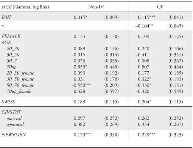
Table 8: Complete Output from the Cost Regression

HCE (Gamma, log link) Non-IV CF

BMI 0.015* (0.009) 0.115*** (0.041)

H –0.104** (0.045)

FEMALE AGE 20_30 30_50 50_7 70up 20_30_female 30_50_female 50_70_female 70up_female 0.135 –0.089 –0.016 0.375 0.850* 0.093 0.031 –0.550*** 0.328 (0.130) (0.136) (0.314) (0.355) (0.445) (0.192) (0.170) (0.209) (0.597) 0.109 –0.240 –0.411 0.008 0.507 0.177 0.322* –0.330* –0.320 (0.125) (0.166) (0.351) (0.362) (0.484) (0.185) (0.183) (0.181) (0.589)

SWISS 0.183 (0.115) 0.204* (0.115)

CIVSTAT married separated 0.297 0.382 (0.252) (0.269) 0.262 0.334 (0.252) (0.267)

(34)

HCE (Gamma, log link) Non-IV CF

ACCIDENT 1.207*** (0.077) 1.203*** (0.078)

CHRONIC 0.874*** (0.068) 0.827*** (0.067)

BACKPAIN 0.081 (0.055) 0.054 (0.053)

WEAK 0.118** (0.058) 0.116** (0.058)

SLEEPING 0.226*** (0.076) 0.228*** (0.074)

HEAD –0.007 (0.058) 0.004 (0.057)

HSTATUS well fair bad very bad 0.227*** 0.942*** 1.775*** 2.276*** (0.068) (0.089) (0.204) (0.665) 0.197*** 0.860*** 1.664*** 2.293*** (0.067) (0.094) (0.214) (0.668) EDUCATION 2 3 4 5 6 7 8 9 10 11 0.041 –0.403** –0.673*** –0.177 –0.338* –0.152 –0.264 –0.126 –0.281 –0.176 (0.138) (0.176) (0.237) (0.164) (0.197) (0.191) (0.201) (0.248) (0.213) (0.194) –0.060 –0.505*** –0.726*** –0.302* –0.350* –0.188 –0.385* –0.147 –0.337 –0.231 (0.121) (0.176) (0.235) (0.160) (0.201) (0.186) (0.197) (0.251) (0.213) (0.191) EMPLOY nonworking unemployed 0.055 0.398* (0.095) (0.241) 0.041 0.241 (0.090) (0.246) URBAN urban suburban 0.008 0.057 (0.091) (0.090) 0.074 0.115 (0.086) (0.086) LANG French Italian 0.135 0.353 (0.119) (0.230) 0.228* 0.276 (0.125) (0.223) Year fixed effects

yes yes

(35)

Table 9: Complete Output from the Outpatient Regression

DOCVIS (Negbin, log link) Non-IV CF

BMI 0.013** (0.005) 0.051** (0.020)

H –0.040* (0.022)

FEMALE AGE 20_30 30_50 50_70 70up 20_30_female 30_50_female 50_70_female 70up_ female 0.173*** –0.130* –0.298* –0.036 0.301 0.102 0.156 –0.123 –0.483 (0.066) (0.075) (0.167) (0.182) (0.240) (0.091) (0.099) (0.103) (0.321) 0.166** –0.184** –0.434** –0.161 0.172 0.124 0.250** –0.057 –0.461 (0.065) (0.083) (0.177) (0.192) (0.260) (0.092) (0.106) (0.106) (0.325)

SWISS 0.101 (0.064) 0.106* (0.063)

CIVSTAT married separated 0.230 0.260 (0.152) (0.162) 0.228 0.252 (0.152) (0.161)

NEWBORN 0.570 (0.357) 0.619* (0.346)

ACCIDENT 0.857*** (0.047) 0.853*** (0.047)

CHRONIC 0.765*** (0.037) 0.749*** (0.037)

BACKPAIN 0.064** (0.030) 0.057* (0.030)

WEAK 0.153*** (0.030) 0.151*** (0.030)

SLEEPING 0.114*** (0.034) 0.115*** (0.034)

HEAD 0.082*** (0.030) 0.086*** (0.031)

(36)

DOCVIS (Negbin, log link) Non-IV CF 10 11 –0.071 –0.027 (0.113) (0.096) –0.084 –0.038 (0.116) (0.098) EMPLOY nonworking unemployed 0.029 0.097 (0.054) (0.132) 0.027 0.049 (0.053) (0.134) URBAN urban suburban 0.059 0.037 (0.053) (0.051) 0.081 0.057 (0.053) (0.049) LANG French Italian 0.195** 0.118 (0.084) (0.128) 0.226*** 0.103 (0.085) (0.129) Year fixed effects

yes yes

Table 10: Complete Output from the Inpatient Regression

HOSPDAYS (Negbin, log link) Non-IV CF

BMI 0.000 (0.017) 0.165** (0.065)

H –0.171** (0.070)

FEMALE AGE 20_30 30_50 50_70 70up 20_30_female 30_50_female 50_70_female 70up_female –0.019 0.012 0.460 1.010* 1.740** –0.015 –0.004 –0.874** 0.065 (0.232) (0.249) (0.544) (0.580) (0.722) (0.392) (0.295) (0.344) (1.014) –0.056 –0.248 –0.278 0.312 1.074 0.128 0.487* –0.503* 0.079 (0.221) (0.291) (0.601) (0.602) (0.769) (0.372) (0.293) (0.298) (0.950)

SWISS 0.096 (0.205) 0.124 (0.205)

CIV_STAT married separated 0.166 0.179 (0.604) (0.629) 0.115 0.107 (0.597) (0.618)

NEWBORN 1.783*** (0.384) 2.055*** (0.385)

ACCIDENT 1.381*** (0.121) 1.373*** (0.122)

(37)

HOSPDAYS (Negbin, log link) Non-IV CF

BACKPAIN 0.042 (0.098) –0.001 (0.095)

WEAK 0.157 (0.103) 0.153 (0.103)

SLEEPING 0.315** (0.126) 0.324*** (0.124)

HEAD –0.177* (0.107) –0.163 (0.107)

HSTATUS well fair bad very bad 0.346*** 1.223*** 2.018*** 2.830** (0.118) (0.148) (0.309) (1.141) 0.292** 1.081*** 1.823*** 2.876** (0.118) (0.155) (0.320) (1.308) EDUCATION 2 3 4 5 6 7 8 9 10 11 0.106 –0.796** –0.932* –0.223 –0.475 –0.201 –0.363 –0.229 –0.428 –0.275 (0.232) (0.373) (0.550) (0.289) (0.386) (0.348) (0.344) (0.433) (0.366) (0.347) –0.060 –0.967*** –1.044* –0.434 –0.472 –0.254 –0.569* –0.222 –0.508 –0.350 (0.203) (0.366) (0.540) (0.278) (0.392) (0.338) (0.336) (0.435) (0.371) (0.340) EMPLOY nonworking unemployed 0.166 0.555 (0.168) (0.410) 0.147 0.267 (0.162) (0.422) URBAN urban suburban –0.225 –0.040 (0.163) (0.157) –0.099 0.066 (0.152) (0.148) LANG French Italian 0.075 0.606* (0.179) (0.367) 0.239 0.455 (0.192) (0.357) Year fixed effects