A R T I C L E
DOI 10.1007/s12651-017-0219-3
Imputation rules for the implementation of the pre-unification
education variable in the
BASiD
Data Set
Nicole Gürtzgen1,2· André Nolte3
Accepted: 11 January 2017 / Published online: 5 April 2017
© The Author(s) 2017. This article is available at SpringerLink with Open Access.
Abstract Using combined data from the German Pension Insurance and the Federal Employment Agency (BASiD), this study proposes different procedures for imputing the pre-unification education variable in the BASiD data. To do so, we exploit information on education-related periods that are creditable for the Pension Insurance. Combining these periods with information on the educational system in the former GDR, we propose three different imputation procedures, which we validate using external GDR census data for selected age groups. A common result from all procedures is that they tend to underpredict (overpredict) the share of high-skilled (low-skilled) for the oldest age groups. Comparing our imputed education variable with information on educational attainment from the Integrated Employment Biographies (IEB) reveals that the best match is obtained for the vocational training degree. Although re-gressions show that misclassification with respect toIEB information is clearly related to observables, we do not find any systematic pattern across skill groups.
Keywords Imputation rules · Administrative data · East Germany · Education · Institutions
Nicole Gürtzgen [email protected] André Nolte
1 Institute for Employment Research, Regensburger Str. 104, 90478 Nuremberg, Germany
2 University of Regensburg, Regensburg, Germany 3 Centre for European Economic Research, Department of
Labour Markets, Human Resources and Social Policy, L 7.1, 68161 Mannheim, Germany
JEL Classification I2 · C81
Imputationsregeln für die Generierung der Bildungsvariable in denBASiD-Daten vor der Wiedervereinigung
Zusammenfassung Der vorliegende Beitrag nutzt admi-nistrative Daten der Deutschen Rentenversicherung und der Bundesagentur für Arbeit (BASiD) um die Bildungsvaria-ble vor der Wiedervereinigung in Ostdeutschland zu impu-tieren. Hierfür werden rentenrechtliche Bildungsperioden genutzt. Anhand der Bildungsperioden und Informationen zum ostdeutschen Bildungssystem werden drei Imputati-onsalgorithmen generiert und mit externen DDR Zensusda-ten validiert. Alle drei Algorithmen unterschätzZensusda-ten (über-schätzten) den Anteil der Hochqualifizierten (Niedrigqua-lifizierten) unter den älteren Personen. Ein weiterer Ver-gleich mit Bildungsinformationen der Integrierten Erwerbs-biographie (IEB) zeigt, dass die größte Übereinstimmung mit Personen aus der Gruppe mit einer Berufsausbildung besteht. Regressionsergebnisse innerhalb der IEB Informa-tionen ergeben des Weiteren, dass eine Missklassifizierung mit beobachteten Variablen korreliert ist. Es bestehen je-doch keine systematischen Zusammenhänge zwischen den Bildungsgruppen.
1 Introduction
long time periods and offering precise longitudinal infor-mation on key variables such as earnings and labour mar-ket states. A further strength of most administrative data sets is that they mitigate problems of panel attrition that typically arise with survey data. In this study, we focus on the 0.25% scientific-use-file of theBASiD(2007) data set (henceforth referred to asBASiD), which supplements a sample of the German Pension Register (VSKT) with information from the Federal Employment Agency.1 The
data provide longitudinal information on individuals’ pen-sion-relevant biographies up to the year 2007. Compared to other administrative data such as theIntegrated Employment Biographies(IEB) from the German Federal Employment Agency,BASiDencompasses entire individual employment biographies (in general starting with the age of 14).
An important feature of the BASiD data set is that it is particularly attractive for studying the Eastern German labour market. While recent studies based on administra-tive data have been highly constrained to the period after unification (see e. g. Kohn and Antonczyk 2013), much of the economic literature dealing with the labour market in the German Democratic Republic (GDR) has relied on the German Socioeconomic Panel (GSOEP) (see e. g. Bird et al.1994).2These survey data provide retrospective GDR
information for the years 1988 and 1989. A great advantage ofBASiDover theGSOEP is that it contains full employ-ment biographies of former GDR citizens prior to German unification. However, a shortcoming of BASiD is that it fails to provide information on individual covariates before 1992 (exceptions are gender and age), including the entire time period prior to unification. Given that especially infor-mation on educational attainment is of major relevance to many labour market applications, this study proposes dif-ferent procedures to impute the pre-unification education variable in theBASiDdata.
While the precision of key variables such as earnings is generally considered to be high, educational information from administrative records is often subject to measurement
1 BASiD is the abbreviation for “Biographiedaten ausgewählter Sozialversicherungsträger in Deutschland”. A larger 1%-sample of the pension part of the data (the sample of the German Pension Reg-ister – VSKT) is available via on-site access at the Research Data Centre of the German Pension Insurance. An alternative version of the fullBASiD1%-sample (including also the data from the Federal Employment Agency) is also available at the Research Data Centre of the Institute for Employment Research (IAB). While the Pension Insurance version provides monthly spell information, the IAB ver-sion provides daily information for all penver-sion relevant episodes (see Hochfellner et al.2012).
2 A further data set is the German Life History Study that sampled five birth cohorts in the former GDR born between 1929 and 1971 (for a documentation see Goedicke et al.2004).
error.3In proposing an imputation procedure for theBASiD
data, our paper is therefore related to the literature dealing with measurement error and missing values (Little and Ru-bin2014, Schafer2010, Manzari2004). While much of the literature on German administrative data has proposed pro-cedures to eliminate inconsistencies (Huber and Schmucker 2009) and to impute missing values of earnings (Büttner and Rässler 2008) or education (Fitzenberger et al. 2006, Wichert and Wilke 2012), our approach has to deal with a complete lack of educational information prior to unifi-cation. Instead of eliminating inconsistencies of an existing variable, we therefore have to provide a rule that indirectly infers educational information from other variables in the data set. We do so by exploiting information on education-related periods that are creditable for the pension insurance (see Table13 in the Appendix). Combining these periods with information on the educational system in the former GDR, we propose three different imputation procedures. The first one, IMP1, attempts to match the six education categories provided by theIEBimposing detailed age con-straints from the institutional information on the GDR ed-ucational system. The second one,IMP2, gives up the age constraints and aims to match somewhat broader education categories, into which the six categories in the IEB have been typically summarised in many empirical applications. Finally, the third one, IMP3, defines the education level based on potential years of education.
We validate our procedures by using external GDR cen-sus data provided by the German Statistical Office (see also Steiner1986and Maaz2002). These data allow us to com-pare the fraction of individuals in specific education-age group cells resulting from our imputations with the cor-responding fractions from the census data for comparable cohorts in 1984. The general picture that emerges is that IMP2andIMP3tend to overpredict the share of medium-skilled workers and underpredict the share of high-medium-skilled for all age groups, whereas they underpredict (overpredict) the share of low-skilled for the younger (older) age groups. The latter is also true for IMP1. Compared with IMP2 and IMP3, IMP1 gives rise to smaller deviations for the share of medium-skilled, whereas it overpredicts the share of high-skilled especially for the younger age groups. Over-all, when balancing out the trade off between goodness of fit and data coverage, the more narrowly defined proce-dureIMP1performs best. However, once one re-classifies those with a GDR Fachschule degree as medium skilled workers, IMP2 is to be preferred over IMP1 and IMP3. After discussing potential sources of misclassification, we
proceed by comparing our education variable prior to unifi-cation with eduunifi-cational information from theIEBright after unification. To do so, we first improve theIEB education information according to the algorithm proposed by Fitzen-berger et al. (2006). For comparison purposes, we then fol-low Wichert and Wilke (2012) by performing a regression analysis in order to identify the importance of observables for a deviation of our imputed educational information from that in theIEB. While misclassification with respect toIEB information is clearly related to observables, we do not find any systematic pattern across skill groups.
The remainder of the paper is structured as follows. Sect. 2 describes theBASiDdata and provides descriptive statistics. Sect. 3 describes the educational system of the GDR and discusses the three imputation rules. Sect. 4 val-idates the imputation results using external census data. Sect. 5 compares the results from our imputations with ed-ucational information from theIEB right after unification. The final Sect. 6 concludes.
2 TheBASiDdata and descriptive statistics
BASiD Data. TheBASiDdata supplement information from the German Pension Register with various data sources from the German Federal Employment Agency. In this con-tribution we use the scientific use file (BASiD-SUF) pro-vided by the German Pension Insurance, which is a strat-ified random 0.25% sample. This data set samples indi-viduals within the age range of 30 and 67, who have an active pension account in 2007. The data therefore com-prise the birth cohorts from 1940 to 1977,4 leading to an
overall sample of about 60,000 individuals. The sample has been drawn in a disproportionate manner and can be made representative using a weighting factor that is part of the data set (for a detailed description see Bönke2009, Him-melreicher and Stegemann2008). To identify former GDR citizens, we first select all individuals who prior to mone-tary union (i. e., the 30th of June 1990) had exhibited at least one monthly spell of pension-relevant activities in the GDR, i. e. those individuals who had gained East German credit points prior to unification. This gives rise to a sam-ple of 11,331 individuals with a total of 2,790,600 monthly spells.
4 The cohort structure of our data implies that the earliest period in which we observe insured individuals is the year 1954, when those born in 1940 were 14 years old. During the subsequent years younger cohorts successively enter the data set, which gives rise to an in-creasingly mixed age structure. To ensure representativeness within the selected cohorts in terms of the working-age population’s age structure, we have constructed weights based upon administrative population data from the German Federal Statistical Office.
The data provide longitudinal information on individ-uals’ entire pension-relevant biographies up to the year 2007. Individual work histories cover the period from the year individuals were aged 14 until the age of 67. Panel attrition may arise only due to individuals’ death or mi-grating abroad. In Germany, statutory pension insurance is mandatory for all employees in the private and public sec-tor, thus only excluding civil servants and self-employed individuals.5 In addition, contributions to the pension
in-surance are paid by the unemployment or health inin-surance during periods of unemployment and prolonged illness.
As stressed at the outset, theBASiDdata provide an ideal basis for analysing labour market related questions of for-mer GDR citizens for several reasons: First, it is the only German administrative data source that encompasses full employment biographies. In particular, thePension Register contains information on all periods for which contributions were paid (employment, apprenticeship training, long-term illness, unemployment) as well as periods without contribu-tions, but which were still creditable for the pension insur-ance. The latter refers to activities for which an individual receives pension credits, such as periods of school or uni-versity attendance after the age of 16 and periods of child rearing and caring.
Second, theBASiDdata is the only individual level data set that contains employment biographies of former GDR citizens before German unification. After unification, for-mer GDR citizens became entitled to transfer their pen-sion-relevant activities to the FRG (Federal Republic of Germany) pension insurance system. For this purpose, the FRG Pension Insurance recorded all periods prior to uni-fication which were creditable for the pension insurance (see above) as well as earnings up to the GDR social se-curity cap. Given that also entitlements from the so called “Freiwillige Zusatzversicherung” could be (partly) trans-ferred to the Western German system, the data cover the full GDR population for whom past pension-relevant peri-ods have been recorded. The pension data therefore allow researchers to track former GDR workers’ entire pre- and post-unification employment histories up to the year 2007. Apart from the individual information on pension-relevant activities and earnings, thePension Registerprovides infor-mation on age and gender.
Starting from 1975 in Western and from 1992 in Eastern Germany, employment spells subject to social security con-tributions from the Pension Register can be merged with data from the German Federal Employment Agency, the IEB and the Establishment History Panel (BHP). The Es-tablishment History Panel contains information on the es-tablishment’s workforce composition, establishment size as
well as sector affiliation (see Table14in the Appendix). Fi-nally, theIEBprovide further time varying individual infor-mation on blue- or white-collar status, occupational status, educational status (see Table15 in the Appendix) and an establishment identifier. A shortcoming of theBASiDdata is therefore that apart from age and gender most covariates (except for those that can be retrieved from the pension-relevant activities listed in Table 13in the Appendix) are available after unification only, starting with the year 1992.
3 Education system in the GDR
Before we turn to our imputation procedures, we provide some institutional background information on the educa-tional system in the former GDR. Due to their common roots the educational systems in the former GDR and West-ern Germany (FRG) exhibit some similarities. However, in the course of the GDR’s history, the systems consider-ably diverged with a strong effect on educational outcomes. While in Western Germany a first selection generally took (and still takes) place during primary school after four years of schooling, GDR students used to spend their first eight years together. Thus, completion of 8th grade may be con-sidered the first official school degree as compared with 9th grade in Western Germany. The completion of 10th grade [referred to as “Polytechnische Oberschule” (POS)] was the second highest formal degree in the former GDR. As will be discussed below, in the 1950s and 1960s only a minority obtained aPOS degree, whereas in later years the majority of students was expected to attend school for
a b
school spells apprenticeship spells
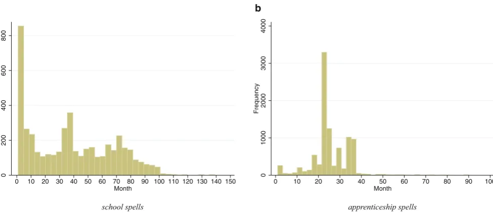
Fig. 1 Distribution of school and apprenticeship spells. (Source:BASiD 2007.Notes:The figure shows the distribution of the length of schooling (a) and apprenticeship spells (b). Schooling spells are coded asses= 1. Apprenticeship spells are coded asses= 2. We close interruptions of type 1 and type 3 (see Table1) if the length of the interruption is less than or equal to six months and if the interruption is not due to a regular employment spell)
ten years (Fuchs–Schündeln and Masella2016). After com-pletion ofPOS, attending high school two more years [re-ferred to as “Erweiterte Oberschule” (EOS)] gave rise to a degree equivalent to the Western German “Abitur” after the completion of the 12th grade. However, as a result from an increasing influence of the “state-governed labour force allocation”, access to high school became highly limited since the late 1960s and was not only determined by stu-dents’ performance but also by their own as well as their parents’ political orientation (Hegelheimer 1973; Huinink and Solga1994).
Regarding the quantitative relevance, the POS degree was of minor importance in early GDR years. In the 1960s, the fraction of students leaving school with 8th grade or less was about 50%. This share decreased gradually, until eventually completion of POS became the most common qualification. At the end of the socialist regime about 80% finished 10th grade (Maaz2002). Restrictive access to high school resulted in a stable low fraction of students complet-ing high school of slightly above 10% (Solga 2002). This development diverged considerably from that in Western Germany, where in 1989 a much higher share had attained lower educational qualification (30%) and a high school degree (25%) (Maaz2002).
a
c
b
total interruptions < 6 month
interruptions ≥ 6 month
Fig. 2 Socio-economic status during the educational interruption. (Source:BASiD 2007.Notes:The figure shows the socio-economic status during the educational interruption. Sub-figureapools all available observations. Sub-figurebconditions on short interruptions defined as those less than six months. Sub-figurecconditions on long interruptions defined as those lasting at least six months or more. See Fig.3for a differentiation by type of interruption)
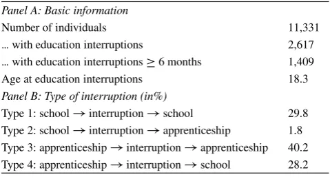
Table 1 Description of the BASiD sample
Panel A: Basic information
Number of individuals 11,331
... with education interruptions 2,617
... with education interruptions6 months 1,409
Age at education interruptions 18.3
Panel B: Type of interruption (in%)
Type 1: school!interruption!school 29.8 Type 2: school!interruption!apprenticeship 1.8 Type 3: apprenticeship!interruption!apprenticeship 40.2 Type 4: apprenticeship!interruption!school 28.2
Source: BASiD2007.
completion of a high school degree, which enabled individ-uals to enter a university afterwards. Given the low share of students with a highest degree of 8th grade or less, in 1987 about 78% of apprenticeship periods exhibited a duration of two years, 11% of 2.5 years and 11% of three years (Fuchs–Schündeln and Masella2016).
univer-a
c d
b
socio-economic status after school socio-economic status after apprenticeship
6 month mode after school 6 month mode after apprenticeship
Fig. 3 Socio-economic status after the eduction period. (Source:BASiD 2007.Notes:The figure shows the socio-economic status after comple-tion of the educcomple-tion period. Sub-figuresaandbfocus on the first month after the eduction period. Sub-figurescanddplot the 6 month mode of the socio-economic status)
sity periods was about four years, on average (Krueger and Pischke1995).
4 Imputation based on educational periods
4.1 Distribution of educational periods
The imputation procedures described in the next section will be basically derived from education-related periods that are creditable for the pension insurance. As spelled out earlier, the Pension Register records periods for which contribu-tions were paid (employment, long-term illness, unemploy-ment) as well periods without contributions, but which are still creditable for the pension insurance, e. g. in terms of waiting times. While vocational training periods generally
include periods with paid contributions, school and univer-sity episodes belong to the second type. By law, the former periods are creditable for the pension insurance of up to 36 months, whereas the latter periods are creditable for the pension insurance for individuals in full time education af-ter the age of 16 for up to 8 years.
To infer information on educational attainment from vo-cational training and schooling episodes, it is instructive to look at the distributions of these spells. A further relevant issue relates to the question as to what extent individuals experienced educational interruptions and what happened during these interruptions. Fig.1displays the distributions of school and apprenticeships spells in our data set.
six years of schooling. The first peak most likely reflects technical school students, whereas the latter peak relates to university graduates.6 Apprenticeship spells are, as
ex-pected, much more concentrated. Most spells last around two years with a further peak at three years. However, there are many spells that lie in between, indicating either mea-surement error, errors that may have occurred when trans-ferring pension entitlements to the Western German pension system or uncompleted spells. Breaking down the descrip-tives by decades (1970s, 1980s, 1990s) shows, however, that the distributions appear to be similar across decades with only some minor differences. In the 1970s, for ex-ample, most of the apprenticeship spells lasted three years compared to the 1990s (see Fig.4for a detailed graphical illustration over time).
Table1shows that among the total number of 11,331 in-dividuals, about 21% (2,414 individuals) experienced some kind of educational interruption. About 46% of the inter-ruptions were rather short. However, 54% of all interrup-tions lasted longer than six months. Breaking down the descriptions by gender shows that females were slightly more likely (58%) to exhibit educational interruptions. On average, the interruptions started at the age of 18.
Panel B distinguishes four types of interruptions. The figures show that most interruptions occurred between two apprenticeship spells. However, with about 28%, there are also sizeable shares of interruptions between two schooling spells (type 1) and those after a period of vocational training followed by a schooling spell (type 4). The distribution does not substantially differ over time and across gender. For males as well as during the 1980s and 1990s, the third type was slightly more prevalent.
A further interesting information stems from the socio-economic status during the interruption and after the com-pletion of the educational period. This may give some hint of whether individuals interrupted an educational episode due to (regular) employment or due to some other reasons, such as sickness absence.
Fig.2a shows that most individuals experienced a reg-ular employment spell during the educational interruption (40%) followed by sickness absence with 37.5%. A third important reason is child rearing with about 12%. In 11% of the interruptions, the socio-economic status is missing. The middle part of the figure shows that for short interruptions (defined as those lasting less than six months), sickness absence was the most common reason followed by child rearing (18.8%) and regular employment (17.9%).
Individ-6 The observation of spells three and six years of schooling may be due to the following reason: Those students who first passed a vocational training degree could enter technical school for three years afterwards. Moreover, students passing EOS (about one year of contribution at the end of EOS) and attending a university for four years afterwards exhibit at least 60 months of contributions.
uals experiencing an interruption longer than six months were primarily in regular employment (78%), whereas for about 22% the socio-economic status is not known. Over-all, these findings suggest that short-term interruptions are mainly interruptions occurring within one (longer) educa-tional spell.
Panel 1 of Fig. 3 shows the distribution of the socio-economic status in the first month after the educational pe-riod. The figure reveals that regular employment is the most frequent status after a school or apprenticeship spell. After schooling periods, the socio-economic status is missing for about 30% of all observations, whereas missing information after an apprenticeship spell is less relevant.
The lower two figures plot the distribution of the main/ dominant socio-economic status within the first six months after the educational period. Also at this stage, the main status is regular employment. Interestingly, missing values after schooling episodes do not matter at all as there is no individual with the dominant status being missing after schooling.
4.2 Imputation rules
In what follows, we propose three different imputation pro-cedures, by combining the length of the educational peri-ods described above with information on the educational system in the former GDR. The first procedure,IMP1, at-tempts to match the six education categories provided by theIEBimposing detailed age constraints from the institu-tional information on the GDR educainstitu-tional system. The six categories include (ND) no vocational and no high-school degree (henceforth referred to as “No degree”), (HS) a high school degree, (VT) a completed vocational training, (VTHS) a completed vocational training plus high school degree, (TUD) a technical university degree and finally, (UD) a university degree. The second one,IMP2, gives up the age constraints and aims to match the broader education categories, into which the six categories in theIEBare typi-cally being summarised in many empirical applications: Ac-cording to these, (1) low-skilled workers are those without any postsecondary degree, (2) medium-skilled workers have a completed apprenticeship training and (3) high-skilled workers obtained a degree from university or a technical university. Our last procedure,IMP3, simply defines these three categories based on potential years of education.7
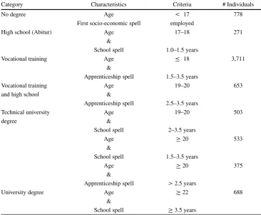
Table 2 Imputation
Proce-dure (1) Category Characteristics Criteria # Individuals
No degree Age < 17 778
First socio-economic spell employed
High school (Abitur) Age 17–18 271
&
School spell 1.0–1.5 years
Vocational training Age 18 3,711
&
Apprenticeship spell 1.5–3.5 years
Vocational training Age 19–20 653
and high school &
Apprenticeship spell 2.5–3.5 years
Technical university Age 19–20 503
degree &
School spell 2–3.5 years
Age 20 533
&
School spell 1.5–3.5 years
Age 20 375
&
Apprenticeship spell >2.5 years
University degree Age 22 688
&
School spell 3.5 years
Source: BASiD2007.
Notes:The total number of individuals under consideration is 11,331. The coverage rate (covered individu-als = 7,026/total individuindividu-als = 11,331) of Imputation Procedure (1) is 62%. Note that the number of covered individuals is less than the sum over all categories because of transitions to a higher educational level. We allow for interruptions of the school and apprenticeship spells and for continuing the spell’s duration after the interruption. See also for a graphical illustration of the procedures and a detailed description of interruptions Appendix B and C. After applying the criteria we extrapolate the educational degree to future spells until we observe a change in individuals’ educational status.
Table 3 Imputation
Proce-dure (2) Category Characteristics Criteria # Individuals
Low-skilled Age 17 778
First socio-economic spell employed
Medium-skilled Apprenticeship >1.5 years 7,845
High-skilled School >3 years 1,374
Source: BASiD2007.
Notes:The total number of individuals under consideration is 11,331. The coverage rate (covered individu-als = 9,634/total individuindividu-als = 11,331) of Imputation Procedure (2) is 85%. Note that the number of covered individuals is less than the sum over all categories because of transitions to a higher educational level. Cu-mulative spells allow for interruptions and for continuing the spell’s duration after the interruption. After applying the criteria we extrapolate the educational degree to future spells until we observe a change in individuals’ educational status.
In general, the three different procedures involve a trade-off between precision and data coverage.IMP1 bears the potential of losing information on individuals who exhibit school or vocational training spells, but not at the required age. By giving up or loosening the age constraints,IMP2 andIMP3 may overcome this loss of observations at the expense of less precision. Table 2 summarises IMP1 im-posing the age constraints (for a graphical summary of the
procedures see also Figure C.1. in the Appendix). For this procedure, we need to know at what ages the different de-grees were typically completed in the socialist system. As documented by Krueger and Pischke (1995), 8th grade and 10th grade were passed at age 14 and 16, respectively. High school was generally completed at age 18.
younger than 17. Note that in this case the skill status may change once individuals have experienced school or ap-prenticeship spells according to the rules spelled out below. We choose an age limit of 17 because students passing an apprenticeship of three years after the 8th grade were on average 17 years old. Thus, even in the case of missing values, the first employment spell should be observed at the age of 17 or older. A student with a high school degree (EOS) should have completed high school at the age of 18 and should exhibit 12 months of schooling in the data. Thus, individuals having experienced a schooling episode between 1 and 1.5 years at the age of 17 or 18 are assigned a high school degree (category (HS) from the IEB). To match categories (VT) and (VTHS) from theIEB, we distin-guish between those with a completed vocational training after 8th or 10th grade and those combining high school with apprenticeship training. Individuals are assigned to category (VT) (8th grade or 10th grade with apprentice-ship) if they have experienced a vocational training spell at the age of 18 or younger with the length of the training lasting between 1.5 and 3.5 years.8
As already mentioned, a further possibility was to com-bine a three year apprenticeship training with the comple-tion of a high school degree. Thus, individuals having ex-perienced an apprenticeship spell lasting between 2.5 to 3.5 years at the age of 19 or 20 are assigned an apprentice-ship plus high school degree (VTHS).
In the IEB data, the high-skilled comprise those with a technical university degree and a university degree. In what follows, we will simply match theIEBtechnical uni-versity degree with a GDR technical school (Fachschule) degree.9Our assignment rule relies on the fact that
comple-tion of aFachschuletook three years, whereas the comple-tion of a university degree took four years on average. To capture the completion of aFachschuledegree after POS, individuals having experienced a schooling episode of at least 2 up to 3.5 years at the age of 19 to 20 are assigned (TUD). The same assignment is made for individuals hav-ing experienced a schoolhav-ing episode of at least 1.5 up to
8 Note that we also assign individuals younger than 17 to category (VT) if they have experienced apprenticeship spells of less than three years to account for the possibility of potential underreporting of vocational training spells in the data set. Moreover, we also allow for vocational training spells of more than 36 months of contributions. After con-sulting the Pension Insurance, they provided us with the information that some so called ’Träger’ might still have reported more than 36 months as vocational training, whereas others might have reported em-ployment. Fig.1also shows few observations with spells lasting longer than 36 months.
9 We will discuss the limitations of such an approach below.
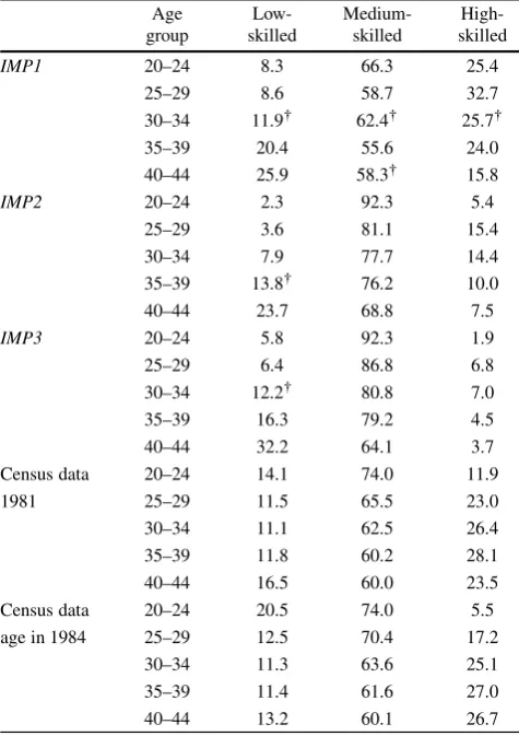
Table 4 Qualification structure by age groups – 1984, I Age group Low-skilled Medium-skilled High-skilled
IMP1 20–24 8.3 66.3 25.4
25–29 8.6 58.7 32.7
30–34 11.9 62.4 25.7
35–39 20.4 55.6 24.0
40–44 25.9 58.3 15.8
IMP2 20–24 2.3 92.3 5.4
25–29 3.6 81.1 15.4
30–34 7.9 77.7 14.4
35–39 13.8 76.2 10.0
40–44 23.7 68.8 7.5
IMP3 20–24 5.8 92.3 1.9
25–29 6.4 86.8 6.8
30–34 12.2 80.8 7.0
35–39 16.3 79.2 4.5
40–44 32.2 64.1 3.7
Census data 20–24 14.1 74.0 11.9
1981 25–29 11.5 65.5 23.0
30–34 11.1 62.5 26.4
35–39 11.8 60.2 28.1
40–44 16.5 60.0 23.5
Census data 20–24 20.5 74.0 5.5
age in 1984 25–29 12.5 70.4 17.2
30–34 11.3 63.6 25.1
35–39 11.4 61.6 27.0
40–44 13.2 60.1 26.7
Source: BASiD2007, weighted statistics.
Notes:Census data cover the residential population in 1981 and are provided as a scientific use file by the German Statistical Office. All statistics are conditional on not being in education at the time of the interview. The first census figures correspond to the year 1981, the interview year. The figures in the lowest panel provide the shares of those who would have been in the respective age groups in 1984. Low-skilled individuals in the census data are individuals without any degree and with a partial completion of a vocational training. Medium-skilled workers include those with a completed vocational training and so-called “Meister”, whereas high-skilled workers consist of those with a technical school degree and a university degree. It is assumed that the working population does not substantially differ from the residen-tial population because of zero unemployment.indicates insignificant differences compared to the census data measured in 1981.
3.5 years at the age of 20 or older.10As we observe a
con-siderable fraction of individuals having experienced an ap-prenticeship period of at least 2.5 years after the age of 20, those individuals are assigned aFachschuledegree as well. This is to account for the possibility that aFachschule de-gree, which was frequently associated with the completion
Table 5 Differences among imputation procedures – 1984, part 1
Differences Q Individuals N Coverage C Q/N Q/C
Sum of squared difference
IMP1 687.5 5,698 0.53 0.121 1297.2
IMP2 2242.7 7,556 0.71 0.297 3158.7
IMP3 3551.9 9,027 0.82 0.393 4331.6
Absolute difference
IMP1 84.1 5,698 0.53 0.015 158.7
IMP2 166.4 7,556 0.71 0.022 234.4
IMP3 204.7 9,027 0.82 0.023 249.6
Source: BASiD2007, weighted statistics.
Notes:Total number of individuals in 1984: 10,702. The sum of square differences and absolute differences are estimated using the age groups in 1981. The coverage rate ofIMP3is rather low because for some individuals the requirements were not met at that point in time.
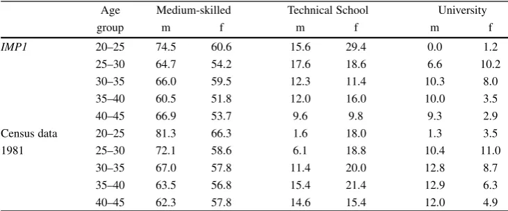
Table 6 Qualification structure by age groups and gender – 1984
Age Medium-skilled Technical School University
group m f m f m f
IMP1 20–25 74.5 60.6 15.6 29.4 0.0 1.2
25–30 64.7 54.2 17.6 18.6 6.6 10.2
30–35 66.0 59.5 12.3 11.4 10.3 8.0
35–40 60.5 51.8 12.0 16.0 10.0 3.5
40–45 66.9 53.7 9.6 9.8 9.3 2.9
Census data 20–25 81.3 66.3 1.6 18.0 1.3 3.5
1981 25–30 72.1 58.6 6.1 18.8 10.4 11.0
30–35 67.0 57.8 11.4 20.0 12.8 8.7
35–40 63.5 56.8 15.4 21.4 12.9 6.3
40–45 62.3 57.8 14.6 15.4 12.0 4.9
Source: BASiD2007, weighted statistics.
Notes:Census data cover the residential population in 1981 and are provided as a scientific use file by the German Statistical Office. It is assumed that the working population does not substantially differ from the residential population because of zero unemployment.
of a vocational training, might have been (mis)reported as a vocational training period in the Pension data.11Finally,
individuals are assigned a university degree (UD) if they have experienced a schooling spell of at least 3.5 years at the age of 22 years or older.
Procedure (2) is summarised in Table 3. Low-skilled workers are those assigned “No degree” (see IMP1). Medium-skilled workers need to have at least 1.5 years of formal apprenticeship training, whereas high-skilled workers are those with school spells of at least three years. The third approach relies on potential years of educa-tion (IMP3). Given that formal unemployment was offi-cially barely present in the GDR12, the idea of this rule is
that the first employment spell should have immediately
11 In the Pension Insurance’s documentation (”Benutzerhinweise zu den sozialen Erwerbssituationen”), vocational training spells may ex-plicitly cover apprenticeship periods, preparatory vocational training measures as well as technical school (”Fachschule”) spells. The latter may also be coded as schooling spells, such that there is some ambigu-ity with respect to technical school episodes.
12 See a discussion by Gürtler et al. (1990) on hidden unemployment.
followed the completion of an educational degree. We de-fine individuals as low-skilled if they are less than 17 years old and are labeled as employed (employment subject to social security contributions excluding apprenticeship peri-ods). Individuals starting employment between 17 and 20 are defined as medium-skilled, whereas high-skilled indi-viduals are those with a first employment spell at the age of 21 to 28. Note that this approach does not account for po-tential changes in educational attainment over individuals’ life courses.13
13 Among the 11,331 individuals in the sample, the fraction exhibit-ing employment as the first state is 11.3%, out of which about 19% returned to education at some later point in time. This accounts for 2.2% of the whole sample. In total, the procedure generates 1,373 low-skilled, 9,089 medium-skilled and 609 high-skilled individuals. The
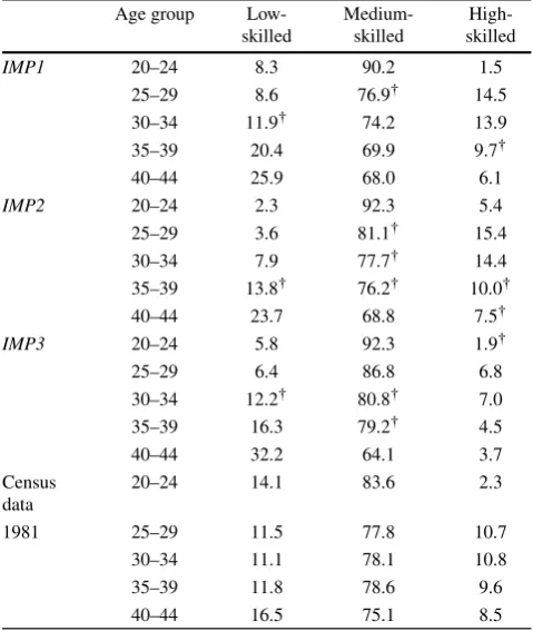
Table 7 Qualification structure by age groups – 1984, II
Age group
Low-skilled
Medium-skilled
High-skilled
IMP1 20–24 8.3 90.2 1.5
25–29 8.6 76.9 14.5
30–34 11.9 74.2 13.9
35–39 20.4 69.9 9.7
40–44 25.9 68.0 6.1
IMP2 20–24 2.3 92.3 5.4
25–29 3.6 81.1 15.4
30–34 7.9 77.7 14.4
35–39 13.8 76.2 10.0
40–44 23.7 68.8 7.5
IMP3 20–24 5.8 92.3 1.9
25–29 6.4 86.8 6.8
30–34 12.2 80.8 7.0
35–39 16.3 79.2 4.5
40–44 32.2 64.1 3.7
Census data
20–24 14.1 83.6 2.3
1981 25–29 11.5 77.8 10.7
30–34 11.1 78.1 10.8
35–39 11.8 78.6 9.6
40–44 16.5 75.1 8.5
Source: BASiD2007, weighted statistics.
Notes:Census data cover the residential population in 1981 and are provided as a scientific use file by the German Statistical Office. It is assumed that the working population does not substantially differ from the residential population because of zero unemployment. The medium-skilled group now includes former technical school graduates.
indicates insignificant differences compared to the Census data
mea-sured in 1981.
5 Qualification structure
This section attempts to externally validate our proposed imputation procedures. To do so, we compare the qualifica-tion structures by age groups obtained from our procedures with those from GDR census data from 1981 for the whole residential population. Note that due to the coverage of the pension data and basically zero unemployment, the working population should not substantially differ from the residen-tial population.
The first three panels in Table4show the imputed quali-fication structures distinguished by five age groups, whereas the last two panels display the figures from the census data. Note that our imputed figures refer to the same age groups three years later in 1984 as the cohort structure of our data set allows us to provide figures for the oldest age group (40–44) only from 1984 onwards. For comparison, the first Census panel reports the shares of all individuals who were within the relevant age groups in 1981. The bottom Cen-sus panel displays the skill shares of those individuals who would have been in the respective age groups in 1984. The
purpose of this comparison is to obtain some information on cohort-specific trends.
The census figures shown in the upper bottom panel in-dicate that the share of low-skilled workers is U-shaped, whereas the share of medium-skilled workers is decreasing with age. For high-skilled individuals, we observe a kind of inverse U-shaped picture with the largest share of high-skilled individuals in the second oldest age group. For the younger age groups, IMP1 assigns substantially more in-dividuals to the high-skilled group compared to the census figures and less to the medium and low-skilled category. For the older age groups, it assigns substantially more in-dividuals to the low-skilled and less to the high-skilled category. IMP2 generates high and low-skilled (medium-skilled) shares that are substantially lower (higher) for most of the age groups than those from the census data. IMP3 leads to an even more pronounced underprediction of the share of high-skilled in all age groups. This reflects that IMP3 does not account for completed school episodes at the age of 21 or younger that might have led to a Fach-schule (technical school degree) after completion ofPOS. Looking at the low-skilled share obtained fromIMP3 sug-gests that the average age of the first labour market spell increased over time. This is due to the fact that the dom-inant school degree moved from 8th grade or less (about 30% of school-leavers had less than 8th grade in the 50s and up to 60% had 8th grade) to the 10th grade over that time period (see for a detailed description Solga2002).
The bottom panel displays the census data of those who would have been in the respective age groups in 1984. This creates substantial deviations for the youngest group, given that some of these individuals were only 17 years old at time of the interview. Because most of the high-skilled in-dividuals were still in the educational system, we observe a higher share of low-skilled and a lower share of high-skilled individuals. This suggests that the comparison is less meaningful for the youngest age group. For the older age groups, however, the pictures does not change substan-tially. Only those in the age group 40 to 44 in 1984 exhibit lower low-skilled and higher high-skilled shares.
Overall, the discrepancies are non-negligible for each of our proposed procedures. To rank the procedures in terms of the implied deviations from the census data, we calculate the sum of squared differences and the absolute differences between the imputed and the census figures over the differ-ent age-skill cells. Table5presents the results.IMP1results in a sum of squared differences equal to 688, whereasIMP2 involves a sum of squared differences equal to 2243. Using IMP3we obtain a number of 3552.
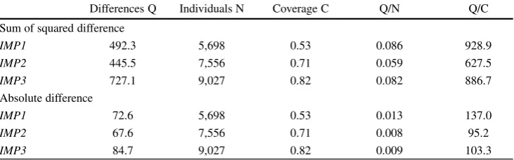
Table 8 Differences among Imputation Procedures – 1984, part 2
Differences Q Individuals N Coverage C Q/N Q/C
Sum of squared difference
IMP1 492.3 5,698 0.53 0.086 928.9
IMP2 445.5 7,556 0.71 0.059 627.5
IMP3 727.1 9,027 0.82 0.082 886.7
Absolute difference
IMP1 72.6 5,698 0.53 0.013 137.0
IMP2 67.6 7,556 0.71 0.008 95.2
IMP3 84.7 9,027 0.82 0.009 103.3
Source: BASiD2007, weighted statistics.
Notes:Total number of individuals in 1989: 11331.
Table 9 Qualification structure by age groups – 1989 Age
group
Low-skilled
Medium-skilled
High-skilled
IMP1 20–24 6.6 90.2 3.2
25–29 5.4 82.1 12.5
30–34 8.4 77.8 13.5
35–39 12.3 75.8 11.9
40–44 20.7 70.3 9.0
Census data 20–24 14.1 83.6 2.3
1981 25–29 11.5 77.8 10.7
30–34 11.1 78.1 10.8
35–39 11.8 78.6 9.6
40–44 16.5 75.1 8.5
Source: BASiD2007, weighted statistics.
Notes:Census data cover the residential population in 1981 and are provided as a scientific use file by the German Statistical Office. It is assumed that the working population does not substantially differ from the residential population because of zero unemployment. The medium-skilled group now includes former technical school graduates.
Dividing Q by the number of individuals (or equivalently by the coverage rate), the ranking stays the same. The same conclusion holds when using absolute differences.
What still remains to be resolved is the question as to why we observe these differences, especially for the share of high-skilled. One possible explanation for the strong de-viations produced byIMP2andIMP3could be that the cen-sus data are biased towards an over-reporting of high-skilled individuals. An alternative explanation could be that there is a reporting error for school and apprenticeship spells in the administrative data set. Regarding the second explana-tion (reporting error) we do not think that this is a major problem as especiallyIMP2andIMP3should also capture those, whose pension accounts in terms of schooling and apprenticeship episodes might have been incomplete.
Moreover, note that even procedureIMP1, which explic-itly attempts to distinguish those with aFachschulefrom those with a university degree, substantially underpredicts (overpredicts) the share of high-skilled especially for the older (younger) age groups. To obtain a more precise pic-ture of potential misclassification sources, we break down
the results fromIMP1by female and male workers as well as by those with a technical school and university degree (see Table 6). The resulting figures show that the way we assigned the education variable performs relatively well for university graduates (for both male and female workers) and medium-skilled male workers as compared to the technical school degree, where large discrepancies can be observed for all age groups.
To account for a potential misclassification of a techni-cal school as a vocational degree, one approach to handle this difficulty could be to re-classify the medium-skilled by assigning all technical school graduates to the medium-skilled. After this re-classification, the high-skilled group would only include university graduates. In terms of the Western German skill categories, such a re-classification could e. g. be justified by the fact that in the GDR individ-uals could enter a technical school after completion ofPOS (Krueger and Pischke1995), which would be rather equiv-alent to a Western German vocational training degree. The results from this re-classification are shown in Table7. The upper part of Table7shows that the share of high-skilled workers decreases and becomes closer to the official data particularly for the older age groups. Thus, treating former Technical Schoolgraduates as medium-skilled may help to draw a somewhat clearer picture for the high-skilled group. The table also shows again the shares generated byIMP2 andIMP3. After the re-classification, for IMP2 six out of 15 cells are not significantly different from the census data. After the re-classification, the sum of squared and ab-solute differences become smaller for all three imputa-tion procedures, with IMP2 and IMP3 showing stronger improvements.14
The ranking of the procedures changes as well. Based on the Q measure and the number of individuals (coverage rate),IMP2is now preferred overIMP3andIMP1.
Given the substantial deviations for the older age groups that result from all three procedures, we next check whether
Table 10 Cross tabulation of
IMP1vs.IEB, I DegreeIMP1
IEB(IP1) Missing ND VT VTHS TUD UD
Missing 33.9 39.7 31.7 32.5 37.8 25.5
ND 4.7 14.1 4.7 3.0 1.5 0.4
VT 56.6 44.7 61.4 56.7 43.7 17.2
VTHS 1.6 0.6 1.0 3.1 6.9 5.8
TUD 2.0 0.5 1.5 3.0 15.3 10.3
UD 1.1 0.1 0.1 1.6 4.5 40.4
Observations 4234 778 3566 573 1103 929
Source: BASiD2007, weighted statistics.
Notes:The categoryHigh schoolplays with 1.3% a minor rule and is not presented in the table. Total number of observations is 11,331. The reference point in time for the comparison is January 1993. Abbreviations: ND: no degree, VT: completed vocational training, VTHS: high school with vocational training. TUD: tech-nical university degree, UD: university degree. In the Pension dataTUDcorresponds to a technical school (Fachschule) degree.
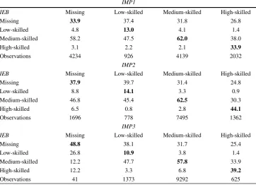
Table 11 Cross tabulation of
IMP1,IMP2andIMP3vs.IEB, II
IMP1
IEB Missing Low-skilled Medium-skilled High-skilled
Missing 33.9 37.4 31.8 26.8
Low-skilled 4.8 13.0 4.1 1.4
Medium-skilled 58.2 47.5 62.0 38.0
High-skilled 3.1 2.2 2.1 33.9
Observations 4234 926 4139 2032
IMP2
IEB Missing Low-skilled Medium-skilled High-skilled
Missing 37.9 39.7 31.4 24.8
Low-skilled 8.8 14.1 3.3 0.9
Medium-skilled 46.8 45.4 62.5 30.3
High-skilled 6.5 0.8 2.8 44.1
Observations 1696 778 7495 1362
IMP3
IEB Missing Low-skilled Medium-skilled High-skilled
Missing 48.8 38.1 31.7 25.4
Low-skilled 26.8 10.9 3.8 1.4
Medium-skilled 12.2 47.7 57.8 33.9
High-skilled 12.2 3.3 6.8 39.2
Observations 41 1373 9292 625
Source: BASiD2007.
Notes:Total number of observations 11,331. The reference point in time for the comparison is January 1993. Abbreviations (IEB): Low-skilled include ND and HS, Medium-skilled include VT and VTHS, High-skilled include TUD and UD.
our procedures are at least able to reproduce the docu-mented decline in the fraction of those leaving school at 8th grade or less. We do this by estimating our skill shares at a later point in time (five years later in 1989). Individu-als from the oldest age group (those aged 44) in 1989 were born in 1945 and were potentially available for the labour market in 1960/1961. Given that the share of those leaving school at 8th grade or less was twice as high in the 1950s as compared to the 1960s (Solga2002), we expect a sharp
de-cline in the predicted low-skilled share especially for older age groups. Table9presents the results forIMP1.
Taken together, our comparison with the census data sug-gests that all three procedures exhibit non-negligible devia-tions from our external data source. In order to finalise our decision about which procedure to use, we further compare our imputation results to information provided by theIEB subpart of the data set.
6 Comparison with educational information from theIEB
We next compare the results from our imputation proce-dures with educational information from the IEB, which can be merged to theBASiD data. Even though the IEB information starts in 1992, we use January 1993 as a refer-ence point as there is evidrefer-ence that education information is more reliable from 1993 onwards. With this comparison we have to keep in mind that theIEBeducation information may be subject to measurement error as well. To mitigate this issue, we correct the IEB education information us-ing the imputation algorithmIP1proposed by Fitzenberger et al. (2006). The authors suggest three different imputation rules without a strict order. The idea behind their rules is based on the assumption that individuals cannot lose their educational degrees. In what follows we useIP1, since ac-cording to Wichert and Wilke (2012) imputation procedure 1 (IP1) leads to a stronger reduction in measurement error. We perform this exercise for all of our imputation pro-cedures. Table10first cross tabulates the results from pro-cedureIMP1using the categories described in Table2with education information from theIEB.
Table10 shows that the best match is obtained for the vocational training (VT) category with a fraction of 61% receiving this category from both our imputation proce-dureIMP1and theIEB. In contrast, among those assigned a vocational training plus high school degree (VTHS) in the Pension data, over 50% exhibit only a vocational training degree (VT) in the IEB. Note that this may either reflect that our imputation procedure wrongly assigns a vocational plus high school degree or, alternatively, that the GDR high school degree has either not been reported or recognised by Western German employers.
Moreover, theIEB comparison also produces large de-viations for those assigned no degree in the Pension data (ND), who mostly exhibit a vocational training (VT) in the IEB. A potential explanation would be that our defined rules from procedureIMP1might have changed over time, such that older workers could have completed an apprenticeship within a shorter duration. If this was the case, the devi-ation of IMP1 from IEB information should be mitigated usingIMP2, as this procedure requires only a cumulative apprenticeship spell of at least 1.5 years. The second panel of Table 11 shows that this does not account for the
ob-served deviation in Table10. In Table11the share of those assigned no degree ND in the Pension data, who exhibit a vocational training (VTand VTHS) in theIEB, remains basically the same for IMP2. Note that the share of low-skilled decreased substantially for all age groups between 1984 and 1989, such that over-reporting a low-skilled sta-tus is unlikely to explain the deviation for the low-skilled in Table10. An alternative explanation would be vocational on-the-job training, which generally cannot be ruled out as a source of any deviation between the (imputed) pension data andIEBinformation.15
Given the problem with correctly assigning the technical school [or technical university degree (TUD)], over 50% of those assignedTUDin the Pension data exhibit only a voca-tional training degree (VTorVTHS) in theIEB. This high-lights again the difficulty in distinguishing between a GDR technical school and a vocational degree. Note that this misclassification might also reflect the fact that educational degrees obtained during GDR times might have not been recognised by Western German employers after unification. The overlap ofTUDwith a university degree (UD) is only moderate with 4.5%.16From the 929 individuals who were
assigned UDin the Pension data, about 40% exhibit also aUDin theIEB. 25% have missing values in theIEBand about 17% intersect with vocational training (VT).
The cross tabulation of the results fromIMP2andIMP3 with education information from the IEBis shown in Ta-ble 11. As these procedures target three education cate-gories – low-skilled, medium-skilled and high-skilled, we also provide the shares for the first imputation procedure IMP1using the three categories in the upper panel.
The picture that emerges from Table 11is that all three procedures show again very similar patterns. The best match is obtained for the medium-skilled, whereas the worst match results for the low-skilled.17Overall, for the 11,331
individ-uals in the BASiDdata set we obtain the highest number of missing values (4,234) for procedure IMP1. The num-ber of missing values in the IEB(3,643) variable is lower compared to IMP1 but twice as large compared to IMP2, indicating a substantial gain in information resulting from
15 We also performed the same analysis with individuals who were unemployed in 1993, with the result of less overlap.
16 This again suggests that re-classifying a Fachschule degree as medium-skilled would potentially reduce measurement error issues and misclassification.
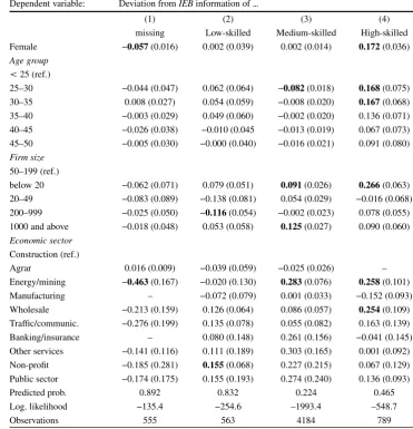
Table 12 Marginal effects of
a logit regression Dependent variable: Deviation fromIEBinformation of ...
(1) (2) (3) (4)
missing Low-skilled Medium-skilled High-skilled
Female −0.057(0.016) 0.002 (0.039) 0.002 (0.014) 0.172(0.036)
Age group
<25 (ref.)
25–30 −0.044 (0.047) 0.062 (0.064) −0.082(0.018) 0.168(0.075)
30–35 0.008 (0.027) 0.054 (0.059) −0.008 (0.020) 0.167(0.068)
35–40 −0.003 (0.029) 0.049 (0.060) −0.002 (0.020) 0.136 (0.071)
40–45 −0.026 (0.038) −0.010 (0.045 −0.013 (0.019) 0.067 (0.073)
45–50 −0.005 (0.030) −0.000 (0.040) −0.016 (0.021) 0.091 (0.080)
Firm size
50–199 (ref.)
below 20 −0.062 (0.071) 0.079 (0.051) 0.091(0.026) 0.266(0.063)
20–49 −0.083 (0.089) −0.138 (0.081) 0.054 (0.029) −0.016 (0.068)
200–999 −0.025 (0.050) −0.116(0.054) −0.002 (0.023) 0.078 (0.055) 1000 and above −0.018 (0.048) 0.053 (0.058) 0.125(0.027) 0.090 (0.060)
Economic sector
Construction (ref.)
Agrar 0.016 (0.009) −0.039 (0.059) −0.025 (0.026) –
Energy/mining −0.463(0.167) −0.020 (0.130) 0.283(0.076) 0.258(0.101)
Manufacturing – −0.072 (0.079) 0.001 (0.033) −0.152 (0.093)
Wholesale −0.213 (0.159) 0.126 (0.064) 0.086 (0.057) 0.254(0.109)
Traffic/communic. −0.276 (0.199) 0.135 (0.078) 0.055 (0.082) 0.163 (0.139)
Banking/insurance – 0.080 (0.148) 0.261 (0.156) −0.041 (0.145)
Other services −0.141 (0.116) 0.111 (0.189) 0.303 (0.165) 0.001 (0.092) Non-profit −0.185 (0.281) 0.155(0.068) 0.227 (0.215) 0.067 (0.129) Public sector −0.174 (0.175) 0.155 (0.193) 0.274 (0.240) 0.136 (0.093)
Predicted prob. 0.892 0.832 0.224 0.465
Log. likelihood −135.4 −254.6 –1993.4 –548.7
Observations 555 563 4184 789
Source:BASiD 2007.
Notes:Robust standard errors are in parentheses. Bold numbers represent significance on at least the 5% level.
our imputation procedures.18As mentioned earlier, there
ex-ists generally a trade-off between precision and coverage in terms of missing values. Given that the main diagonal val-ues are largest forIMP2, which simultaneously reduces the number of missing values by almost 50%, procedureIMP2 seems to provide a quite reasonable compromise between matchingIEBinformation and data coverage.
To analyse whether any deviation fromIEBinformation is systematically related to observables, we next perform a logit analysis using the results from procedure (IMP2) for the year 1993. The dependent variable is one if the edu-cational degree assigned in the Pension data deviates from the educational information in theIEB and is zero other-wise. Table12 presents the estimated marginal effects for the probability of misclassification in the pooled sample
18 Missing values in the IEB part of the data set are with 4,204 missing entries substantially higher in 1992.
significant. The signs of the marginal effects of different industry affiliations do not reveal any systematic pattern either and also vary greatly across skill groups.
7 Conclusions
TheBASiDdata set provides the only available data source that contains full employment biographies of former GDR citizens prior to German unification. However, a shortcom-ing ofBASiDis that it fails to provide information on indi-vidual covariates prior to unification (exceptions are gender and age). Given that especially information on educational attainment is of major relevance to many labour market ap-plications, this study proposes different procedures to im-pute the pre-unification education variable in the BASiD data.
Our proposed procedures exploit information on edu-cation related periods that are creditable for the pension insurance. Combining these periods with information on the educational system in the former GDR, we investi-gate three different imputation procedures. The first one, IMP1, attempts to match the six education categories pro-vided by theIEB imposing detailed age constraints from the institutional information on the GDR educational sys-tem. The second one, IMP2, gives up the age constraints and aims to match somewhat broader education categories, into which the six categories in the IEB have been typi-cally summarised in many empirical applications. Finally, the third one,IMP3, defines the education level based on potential years of education.
We validate our procedures by using external GDR cen-sus data provided by the German Statistical Office. These data allow us to compare the fraction of individuals in specific education-age group cells resulting from our im-putations with those from the census data for comparable cohorts in 1984. The general picture that emerges is that IMP2andIMP3 tend to overpredict the share of medium-skilled workers and underpredict the share of high-medium-skilled
for all age groups, whereas they underpredict (overpredict) the share of low-skilled for the younger (older) age groups. The latter is also true forIMP1. Compared withIMP2and IMP3,IMP1gives rise to smaller deviations for the share of medium-skilled, whereas it overpredicts the share of high-skilled especially for the younger age groups. Overall, when balancing out the trade off between goodness of fit and data coverage, the more narrowly defined procedureIMP1 per-forms best.
Finally, a comparison of our (imputed) education infor-mation prior to unification with educational inforinfor-mation from theIEBright after unification suggests that the best fit is obtained for those assigned a vocational training degree in the Pension data. The largest discrepancy is observed for those assigned a technical university degree in the Pen-sion data of whom a large fraction (over 50%) exhibits only a vocational training degree in theIEB. This highlights again the difficulty in distinguishing between a GDR Fach-schuleand a vocational training degree. A simple approach to handle this difficulty could be to redefine the medium-skill category by assigning all technical (school) university graduates to the medium-skilled, such that the high-skilled group would only include university graduates. After doing so,IMP2would be preferred overIMP1andIMP3. Given thatIMP2simultaneously gives rise to the least number of missing values and provides the best match to theIEB in-formation, our proposed procedureIMP2seems to provide a quite reasonable compromise between matching external information and data coverage.
Acknowledgements We would like to thank Sebastian Butschek, Laura Pohlan and three anonymous referees for helpful comments and suggestions. We further thank Maria Bidenko and Vanessa Linden-maier for providing excellent research assistance.
Appendix
Appendix A: Data description
Table 13 Description of individual employment history variables gained from the
Pension Register
Variable1) Definition SES Coding2)
EMPLOYMENT Employment spells include periods of employ-ment
13 subject to social security contributions and
(after 1998) marginal employment.
UNEMPLOYMENT Unemployment spells include periods of 6, 7, 8 unemployment with and without transfer
receipt (only FRG).3)
NON-EMPLOYMENT Non-employment spells include periods of 3, 4 child raising, care giving as well as periods
with missing information on the employment status.
ILLNESS Illness spells include periods of long-term illness 5 (FRG>6 weeks; GDR>4 weeks before 1984, no
minimum restriction afterwards).
TRAINING Training spells include periods of school or 1, 2 university attendance after the age of 16 and
periods of training and apprenticeship.
1)Note that the recorded pre-unification pension activity histories are less precise than the post-unification histories. The reason is that the transfer of the activities was mainly based on former GDR citizens’ social security cards. These cards record the number of months of employment, illness and maternity leave during a particular year, but do not allow for tracking these spells on a monthly basis. As a result, compared to the pension spells after Unification, which provide exact monthly information on all pension relevant activities, information on the incidence of pre-unification employment, illness and maternity leave spells is available only on an annual basis.
2)Further possible states of the SES variable are: Military service (SES = 9), Retirement (SES = 15) and “Else” (SES = 12).
3)A spell of unemployment in thePension Register requires individuals to be registered as unemployed
Table 14 Definition of establishment characteristics gained from the
Employment Statistics Register
Variable Definition/categories: Establishment size Size<20
20Size<50 50Size<200 200Size<1000
Size1000
Workforce Share of employees younger than 30 years composition Share of employees older than 50 years
Share of low-skilled employees Share of female employees Sector affiliation Agriculture/forestry
Mining and manufacturing Energy/water supplies Construction
Wholesale and retail trade Transport and communication Financial intermediation Other service activities Public administration
Table 15 Definition of individuals characteristics Variable/categories Definition
GDR-spell GDR spells are identified based
on the
regional origin (Beitrittsgebiet) of the
pension contributions Educational status 6 categories
NO DEGREE (ND) No high school, no vocational degree
HIGH SCHOOL High school degree (Abitur)
VOC. TRAINING (VT) Completed vocational training VOC. TRAINING + HIGH
SCHOOL (VTHS)
Completed vocational training plus
high school
TECH. UNIVERSITY (TUD) Fachschule or Technical Univer-sity
Degree
UNIVERSITY (UD) University degree Educational status 3 categories
LOW-SKILLED No degree or high school degree MEDIUM-SKILLED Completed vocational training HIGH-SKILLED Technical college degree or
university degree Origin of credit points
“Beitrittsgebiet” (GDR) Variable RCEG = 6
Appendix B: Distribution of education spells and interruptions
a
c d
e f
b
School spells 1970s School spells 1980s
School spells 1990s Apprenticeship spells 1970s
Apprenticeship spells 1980s apprenticeship spells 1990s
Appendix C: Graphical illustration ofIMP 1
References
Biermann, H.: Berufsausbildung in der DDR: Zwischen Ausbildung und Auslese. Springer, Berlin (2013)
Bird, E.J., Schwarze, J., Wagner, G.G.: Wage effects of the move to-ward free markets in East Germany. Ind Labor Relat Rev47(3), 390–400 (1994)
Bönke, T.: Gekappte Einkommen in prozessgenerierten Daten der Deutschen Rentenversicherung – Ein paretobasierter Imputation-sansatz. DRV-Schriften, vol. 55., pp 214–230 (2009)
Büttner, T., Rässler, S.: Multiple imputation of right-censored wages in the German IAB employment sample considering heteroscedas-ticity. Technical report. IAB Discuss Pap44, 22 (2008)
Card, D., Kluve, J., Weber, A.: Active labour market policy evalua-tions: A meta-analysis. Econ J120(548), F452–F477 (2010) Fitzenberger, B., Osikominu, A., Völter, R.: Imputation rules to
im-prove the education variable in the IAB employment subsample. J Appl Soc Sci Stud126(3), 405–436 (2006)
Fuchs–Schündeln, N., Masella, P.: Long-lasting effects of socialist ed-ucation. Rev Econ Stat98(3), 428–441 (2016)
Goedicke, A., Lichtwardt, B., Mayer, K.U.: Dokumentationshandbuch Ostdeutsche Lebensverläufe im Transformationsprozeß: LV-Ost Nonresponse. Max-Planck-Institut für Bildungsforschung, Berlin (2004)
Gürtler, J., Ruppert, W., Vogler–Ludwig, K.: Verdeckte Arbeit-slosigkeit in der DDR. CESifo Group, München (1990). Nr. 100219900050000
Hegelheimer, A.: Berufsausbildung in der DDR – Versuch einer Ein-schätzung. Gewerksch Monatsh24(3), 189–193 (1973)
Himmelreicher, R., Stegemann, M.: New possibilities for socio-eco-nomic research through longitudinal data from the Research Data Centre of the German Federal Pension Insurance. J Appl Soc Sci Stud128(4), 647–660 (2008)
Hochfellner, D., Müller, D., Wurdack, A.: Biographical data of social insurance agencies in Germany – Improving the content of admin-istrative data. Schmollers Jahrb132, 443–451 (2012)
Huber, M., Schmucker, A.: Cleansing procedures for overlaps and inconsistencies in administrative data. The case of length of un-employment in German labour market data. Hist Soc Res 34, 230–241 (2009)
Huinink, J., Solga, H.: Occupational opportunities in the GDR: A priv-ilege of the older generations? Z Soziol23(3), 237–253 (1994) Kohn, K., Antonczyk, D.: The aftermath of reunification. Econ
Transi-tion21(1), 73–110 (2013)
Krueger, A.B., Pischke, J.-S.: A comparative analysis of East and West German labor markets: before and after unification. In: Freeman und Katz: differences and changes in wage structures,
pp. 405–446. University of Chicago Press, Chicago and London (1995)
Little, R.J.A., Rubin, D.B.: Statistical analysis with missing data. John Wiley & Sons, Hoboken, New Jersey (2014)
Kai Maaz. Ohne Ausbildungsabschluss in der BRD und DDR: Berufs-zugang und die erste Phase der Erwerbsbiographie von Ungelern-ten in den 1980er Jahren.Working Paper of the Independent Re-search Group of Max-Planck-Institute for Educational ReRe-search No. 3/2002, No. 3/2002, 2002.
Manzari, A.: Combining editing and imputation methods: an experi-mental application on population census data. J R Stat Soc Ser A
167(2), 295–307 (2004)
Schafer, J.L.: Analysis of incomplete multivariate data. CRC press, Boca Raton London (2010)
Solga, H.: Jugendliche ohne Schulabschluss und ihre Erwerbsbi-ografien. In: Schnabel (ed.) Das Bildungswesen in der Bundesre-publik Deutschland. Strukturen und Entwicklungen im Überblick. Rowohlt Taschenbuch Verlag, Reinbek (2002)
Steiner, I.: Struktur der Allgemeinausbildung und Berufsausbil-dung der Wohnbevölkerung in der DDR – Berufs- und Bil-dungsweglaufbahnen von Schulabsolventen. Akademie der Päda-gogischen Wissenschaft der DDR, Berlin (1986)
Wichert, L., Wilke, R.A.: Which factors safeguard employment?: An analysis with misclassified German register data. J R Stat Soc Ser A175(1), 135–151 (2012)
Nicole Gürtzgen has been head of the IAB research department “Labour market processes and institutions” since October 2015. She also holds a professorship in economics with a focus on labour market research at the University of Regensburg. Prior to her appointment at IAB she held a position as a Senior Researcher at the Centre of Euro-pean Economic Research (ZEW) in Mannheim. From 1990 to 1996, she studied mathematics and economics at the Universities of Duisburg and Heidelberg. After graduating from the University of Heidelberg with a diploma in economics, she completed her doctoral dissertation at the University of Rostock in April 2002. In 2008, she finished her postdoctoral thesis (Habilitation) at the University of Mannheim.