O R I G I N A L A R T I C L E
Open Access
An efficient data structure for calculation of
unstructured T-spline surfaces
Wei Wang
*, Yang Zhang, Xiaoxiao Du and Gang Zhao
Abstract
To overcome the topological constraints of non-uniform rational B-splines, T-splines have been proposed to define the freeform surfaces. The introduction of T-junctions and extraordinary points makes it possible to represent arbitrarily shaped models by a single T-spline surface. Whereas, the complexity and flexibility of topology structure bring difficulty in programming, which have caused a great obstacle for the development and application of T-spline technologies. So far, research literatures concerning T-T-spline data structures compatible with extraordinary points are very scarce. In this paper, an efficient data structure for calculation of unstructured T-spline surfaces is developed, by which any complex T-spline surface models can be easily and efficiently computed. Several unstructured T-spline surface models are calculated and visualized in our prototype system to verify the validity of the proposed method.
Keywords:T-splines, Non-uniform rational B-splines, Unstructured T-mesh, Extraordinary points
Introduction
With a series of excellent mathematical and algorithmic properties, non-uniform rational B-splines (NURBS) has been widely used in the field of computer aided geometric design for representing curves and surfaces. Nevertheless, in modern industry, complex engineering models comprised of multiple NURBS patches are always not watertight because of the existence of gaps and overlaps along the interfaces of trimmed NURBS surfaces. Thus, T-splines were firstly
pro-posed by Sederberg et al. [1,2] in 2003 to conquer the
limi-tations of NURBS in practical engineering applications. As a generalization of NURBS, T-splines introduce T-junctions and extraordinary points into its control mesh. Theoretically, a T-spline surface can represent any arbitrarily shaped model no matter how complicated its topology structure is. Compared with NURBS, the advan-tages of T-splines can be reflected in the following aspects. Firstly, a NURBS surface is defined in a rectangular topo-logical grid. It requires a large number of superfluous con-trol points to maintain the topological shape while implementing refinement. This shortcoming can be over-come by T-splines which can achieve local refinement without introducing an entire row of control points. In
addition, it is difficult to represent a complex model with a single NURBS surface and the gaps along the common boundary of two NURBS surfaces are unavoidable. T-splines provide a promising way to breakdown these barriers. In ref. [3], multiple trimmed NURBS patches are merged into a single watertight T-spline surface. Li et al.[4] studied the linear independence of T-spline blending functions and proposed the notion of analysis-suitable T-splines. Analysis-suitable T-splines satisfy a simple topo-logical requirement and their blending functions are linear independent [4–6]. So far, T-splines have been used in many fields such as geometric modeling [7–9], isogeo-metric analysis [10–15] and shape optimization [16–18].
In complex T-spline models, the extraordinary points are always indispensable. T-splines containing extraor-dinary points are called the unstructured T-splines [14]. When encountering an unstructured T-spline surface, the knot interval vectors about the vertexes around the extraordinary points are ambiguous. More details about the concept of extraordinary points are presented in sec-tion 2. Some methods have been developed to deal with
the problems caused by extraordinary points [14, 19,
20]. In the template method proposed by Wang et al. [19], gap-free T-spline surfaces are generated by insert-ing zero-interval edges around the extraordinary points. Liu et al. [20] proposed a knot interval duplication and
© The Author(s). 2019Open AccessThis article is distributed under the terms of the Creative Commons Attribution 4.0 International License (http://creativecommons.org/licenses/by/4.0/), which permits unrestricted use, distribution, and reproduction in any medium, provided you give appropriate credit to the original author(s) and the source, provide a link to the Creative Commons license, and indicate if changes were made.
* Correspondence:[email protected]
optimization method to obtain local knot vectors. In ref. [14], Scott et al. introduced a linear interpolation scheme to calculate Bézier control points from T-spline control points, which is easy to understand and implement.
Since T-spline surfaces have flexible topology, con-structing a robust and efficient data structures of T-splines for storing and further data processing is a challenging topic. Asche et al. [21] presented a T-spline data structure implementation based on a half-edge (HE) data structure and implemented the algorithms with CGAL geometry programming library. Lin et al. [22] developed the so-called extended T-mesh which can
be represented in an obj-like format file and converted
into the face-edge-vertex data structure conveniently. With this method, each vertex in the extended T-mesh has a knot coordinates, which cannot solve the situtation with extraordinary points. Xiao et al. [23] also proposed a set of new T-spline data models to obtain better data storing and operating efficiencies. However, all the T-spline data structures mentioned above cannot deal with the T-splines with extraordinary points, i.e., un-structured T-splines. To the best knowledge of the au-thors, there are no public research papers or open sources which directly present the suitable approaches to handle the unstructured T-splines from a view of pro-gramming implementation.
In this paper, a new data structure for the unstructured T-splines is proposed. An efficient local parameterization algorithm which can accelerate the computation of T-spline surface is also presented. Finally, several testing examples of unstructured T-splines are demonstrated to show the validity of the proposed data structures and algorithm.
The rest of the paper is organized as follows. In sec-tion 2, we give a brief introducsec-tion of T-splines and ex-plain the concept of extraordinary points. Section 3 is devoted to present the new data structure. In section 4, we give the local parameterization algorithm. Finally, complicated T-spline models are demonstrated in sec-tion 5.
T-splines
A brief introduction of T-splines is reviewed in this sec-tion. We give a description of some symbols and nota-tions appear below as well. In this paper, we only consider bicubic T-splines.
T-mesh
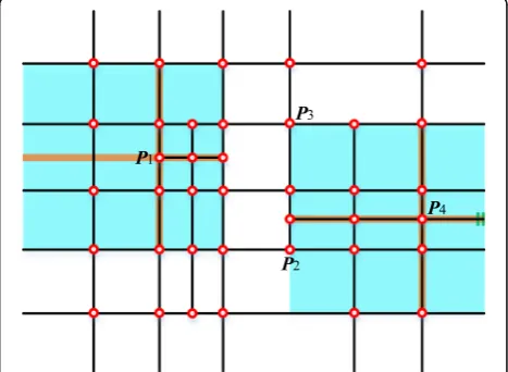
The T-mesh that contains the underlying topology infor-mation is a fundamental concept of a T-spline surface.
As the example shown in Fig.1, a T-mesh is composed
of faces, edges and vertexes. For bicubic T-splines, a control point and related weight are aligned to each
ver-tex in the T-mesh. The T-junctions such asP1and P2in
Fig. 1 make the topological structure of T-splines very
flexible. After a valid knot interval configuration being assigned to the edges, the topology information of T-splines is determined.
T-spline blending function
Each vertex in a T-mesh corresponds to a T-spline blending function. We can construct the blending func-tion from the knot interval sequences inferred from the T-mesh. These knot interval sequences are called local knot interval vectors.
The principles about how to deduce the local knot interval vectors from the T-mesh are presented in refs. [24,25] in detail. In summary, as the brown lines shown
in Fig.2, marching through the T-mesh in four different
topological directions until two vertices or perpendicular edges are detected, the knot interval vectors can be de-termined by the traversed distance. In normal condi-tions, the knot interval is set to be be 0 if a T-mesh
Fig. 1A T-mesh
boundary is crossed. The process of constructing local
knot interval vectors forP1andP4is shown in Fig.2.
As the example shown in Fig. 2, the influence domain
which is called local blending function domains (the blue regions) corresponding to the control points can be de-fined after achieving the knot interval vectors. Then we can set up a local blending coordinate system attached to corresponding vertexes. If there exists no extraordinary point in a T-mesh, a larger global parametric coordinate system can be established which can help us compare dif-ferent blending functions in a common coordinate system.
The global parametric system of the T-mesh in Fig.1
is shown in Fig.3. Each vertex has only one pair of
cor-responding parameter coordinates. However, in the un-structured T-splines which contain extraordinary points, the situation is completely different and that is the main difficulty of constructing an efficient T-spline data structure.
The equation of a T-spline surface can be expressed as:
T¼
Pn
i¼1PiωiNiðμ;νÞ Pn
i¼1ωiNiðμ;νÞ
where Pi are control points, ωi are weights, and Ni are
blending functions,μandνare knot values.
Extraordinary points
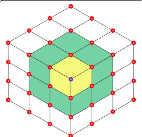
In some T-spline models such as the cube shown in Fig.4, the existence of extraordinary points is inevitable. There are eight extraordinary points on the corners of the cube.
In a T-mesh, the valence of a vertex is the number of edges that touch the vertex. As the T-mesh shown
in Fig. 2, the T-junctions P1 and P2 have three
va-lences. The definition of extraordinary point is that an interior vertex that is not a T-junction and of
which the valence is not equal to 4 [14]. Spoke edge is the edge connected to the extraordinary point. The one-ring neighborhood of a vertex refers to the T-mesh faces which touch the vertex. The faces that touch the one-ring neighborhood form the corre-sponding vertex’s two-ring neighborhood. The T-mesh around the extraordinary point in the purple region
in Fig. 4 is shown in Fig. 5.
In Fig. 5, the valence of the extraordinary point
marked by purple circle is 3. The one-ring neighborhood is represented by yellow and the two-ring neighborhood is represented by green. From the unstructured T-mesh, we can see that it is impossible to set up a common
Fig. 3A global parametric coordinate system
Fig. 4A cube T-spline model. An extraordinary point is marked in the purple region
global coordinate system due to the existence of the extraordinary point, which brings problems to the knot interval vectors definition in their neighborhood.
Data structure for unstructured T-splines
Owing to the fact that extraordinary points are unavoid-able in complicated models, we should reconsider the existing T-spline data structures because with extraor-dinary point appearing it is impossible to assign each vertex a parameter coordinate in a common global para-metric coordinate system.
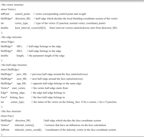
The new data structure we proposed is inspired by the classical HE data structures. Since this data structure provides efficient retrieval of the topological information
associated with the mesh, we can make some modifica-tions to it to meet the requirements of storage and com-putation of the unstructured T-splines.
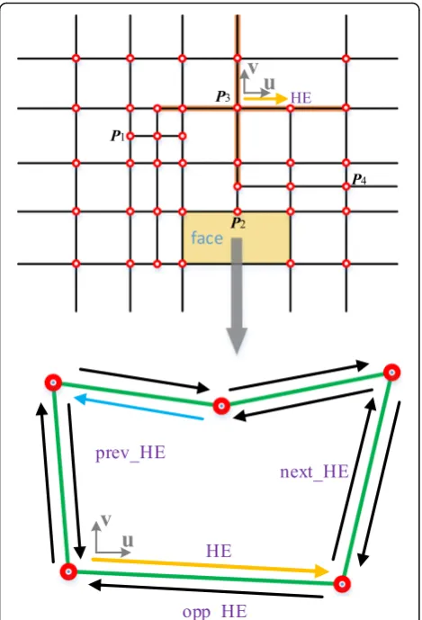
The schematic of the proposed data structure (Table1) is
illustrated in Fig.6. The face marked in yellow region in the
upper T-mesh is composed of five HE. The HEs are denoted by colorful arrows and the green lines represent edges. An edge corresponds to two opposite HEs. Each HE starts from a vertex. What calls for special attention is that in the un-structured T-mesh, a HE doesn’t have a specific direction and a vertex doesn’t have a corresponding global parameter coordinate. This is the main difference between the proposed data structure and those constructed in a global coordinate system.
To facilitate the calculation of the faces in an unstruc-tured T-mesh, a local coordinate system is established
for each face. As the example shown in Fig. 6, the HE
denoted by yellow is chosen to act as theu direction of
the face coordinate system. To make the calculation of the faces more convenient, we can choose any HEs de-noted by a black arrow inside the face to set up the face parametric coordinate system, with the exception of the one starts from a T-junction (the HE denoted by blue in Fig.6).
In order to save in-time computations of the T-spline surface, some redundant data or pointers are stored in the data structure. In order to search the vertexes that have an impact on the faces in the T-mesh, it is essential to select a HE to set up a local blending coordinate sys-tem for each vertex (such as the local blending
coordin-ate system of P3 in Fig. 6). For the faces, the infected
vertexes and their relative coordinates in face coordinate systems are stored in the data structure.
Computation of the unstructured T-splines
An efficient data structure must not only be flexible for data storing but also suitable for the development of re-lated algorithms. In this section, we present an efficient algorithm for the computation of the unstructured T-splines based on the proposed data structure.
Because the faces in a T-mesh have one-to-one map-ping relations with the patches in a T-spline surface, we can tessellation the T-spline surface face by face. The computation of the T-spline surfaces can be summarized as the following steps.
Table 2Local parameterization algorithm
Step 1: Load the T-spline models. In this paper, the T-spline models are constructed in Rhinoceros and
saved asTSM-files.
Step 2: Construct the T-spline data structures.
Step 3: For each vertex, establish a local blending co-ordinate system in the parametric domain after obtain-ing the local knot interval vectors, as the example shown in Fig.2.
Step 4: Find all the faces that overlap the local para-metric domain of the vertex. Then obtain the coordinate of the vertex in different face parametric coordinate systems.
Step 5: For each face find in step 4, add the vertex and coordinate into the face data structure.
Step 6: Compute the T-spline surface face by face by the computation formula.
In the unstructured T-splines, most of the time is spent on step 4 during the surface computation due to the lack of a global parametric coordinate system. Here we give an
effi-cient algorithm called local parameterization (Table 2)
Fig. 7Initial half-edges in the local parametric algorithm
Fig. 8Schematic of the local parametric algorithm
which can improve the efficiency of the calculation of T-spline surfaces.
The main idea of the local parameterization algorithm is to traverse all faces in the local blending function do-main of each vertex and then obtain the coordinate of the specific vertex in face coordinate systems. In the al-gorithm, the whole traversal process of the domain is re-alized from four directions represented by eight HEs. These HEs can be obtained during the procedure of obtaining the local knot interval vectors. If the vertex is
a T-junction such as P1 shown in Fig. 7, we should
change the virtual HE marked by red dashed arrows to the black solid arrows. The eight arrows (in black) are the initial HEs.
To complete the traverse process, if a half-edge HE
is popped from the stack S in line 3 of the algorithm,
we should judge whether the face F it belongs to
overlap the blending function domain Diof the vertex
Pi. In that case, the vertex Pi and its coordinate in
face F’s coordinate system should be added into the
data structure of F firstly. Then the half-edges called
upper-HEs which parallel to HE and belong to the
faces above F should be pushed into the stack S. In
this way, we can make sure that all faces in the blending function domain can be traversed without any omissions.
As the unstructured T-spline with an extraordinary
point P4shown in Fig.8, assume that the orange arrow
starting fromP5is the u direction of the local blending
coordinate system of P5 and the red arrow represents
theudirection of the face coordinate system denoted by
yellow region. The parameter length of the two
HEs marked by green and red are x and y, respectively.
After the initialization, if the HE denoted by green is popped up from the stack, we can see the face (yellow region) it belongs to obviously overlap the local blending domain marked in blue. In the face coordinate system,
the parametric coordinate of P5 is (0, x). Then P5 and
the coordinate should be added into the face data
struc-ture because P5 has an effect on the calculation of the
yellow face. According to the content described in line 8 of the local parameterization algorithm, two HEs
de-noted by purple arrows (upper-HEs mentioned above)
should be pushed into the stack. Thus, we can accom-plish the algorithm by repeating this process. The
par-ameter coordinate of the vertex P5 in different face
coordinate systems is easy to obtain through the connec-tions between the half-edges.
In the neighborhood of the extraordinary points (the
grey and green regions around P5 in Fig. 8), the knot
interval vectors definition is a little tricky. Many
litera-tures have studied on this topic [19, 20,26]. In order to
ensure continuity of the elements near the extraordinary points for further application such as isogeometric ana-lysis, in this paper, we choose the method proposed by Scott et al. [14] to solve this problem. Through the method described in ref. [14], two-ring neighborhood
el-ements are C2 with adjoining three-ring neighborhood
elements, and C1 with their other neighbors; and
one-ring neighborhood elements are G1 with adjoining
one-ring neighborhood elements and C1with adjoining
two-ring neighborhood elements.
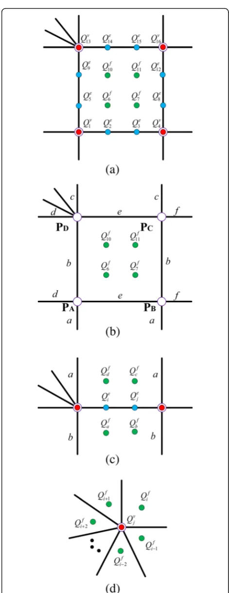
In the two-ring neighborhood of an extraordinary point, the faces can be represented by the linear combi-nations of the T-spline control points. They can be
cal-culated as patches of Bézier elements and the
procedure is simply described in Fig.9. Each bicubic
el-ements contains 16 Bézier control points which can be classified into face points (solid green circles), edge points (solid blue circles) and vertex points (solid red
circles). Each face point denoted by a superscript fcan
be represented in terms of T-spline control points
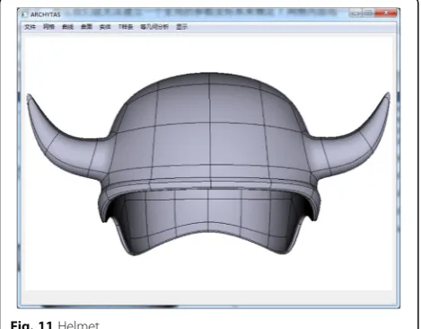
Fig. 11Helmet
(denoted by purple circles). Each edge point denoted by
a superscript e is written in terms of face points and
each vertex point denoted by a superscript v is
repre-sent by the face points. The formulas are defined as.
Q6f¼
bþc aþbþc
eþf dþeþf
PAþ bþc
aþbþc
d dþeþf
PB
þ a
aþbþc
d dþeþf
PCþ a
aþbþc
eþf dþeþf
PD
Q7f¼
bþc aþbþc
f dþeþf
PAþ bþc
aþbþc
dþe dþeþf
PB
þ a
aþbþc
dþe dþeþf
PCþ a
aþbþc
e dþeþf
PD
Q10f ¼
c aþbþc
eþf dþeþf
PAþ c
aþbþc
d dþeþf
PB
þ aþb
aþbþc
d dþeþf
PCþ aþb
aþbþc
eþf dþeþf
PD
Q11f ¼
c aþbþc
f dþeþf
PAþ c
aþbþc
dþe dþeþf
PB
þ aþb
aþbþc
dþe dþeþf
PCþ aþb
aþbþc
f dþeþf
PD
Qe i¼
a aþb
Qf
aþ
b aþb
Qdf
Qe j¼
a aþb
Qbfþ b
aþb
Qf c Qv j¼ XN i¼1
ai−1
ai−1þaiþ1
aiþ2 aiþaiþ2
Qif
Results and discussion
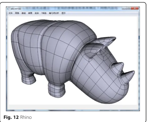
In this section, as given in Figs.10,11,12, and13some
T-spline models are shown to verify the feasibility of the proposed data structures and the local parameterization algorithm. All the models are built from unstructured T-splines which include the extraordinary points except for the gearbox. We can download them from the offi-cial site of Rhinoceros [27].
Conclusion
In this paper, an efficient data structure for the unstruc-tured T-splines is proposed. With this data structure, the topology information of the T-splines can be accur-ately stored. In addition, a valid local parameterization algorithm which can improve the efficiency of the calcu-lation of T-spline surfaces is developed. Some unstruc-tured T-spline surface models are presented to verify the feasibility of data structures. All the data structures and algorithms presented in this paper have been imple-mented in our CAD/CAE/OPT integration software Archytas. In the future, the local refinement and the other correlative algorithms will be developed based on the proposed data structures.
Abbreviations
HE:Half-edges; NURBS: Non-uniform rational B-splines
Acknowledgements
The authors would like to acknowledge the support by the National Natural Science Foundation of China (Nos. 61572056 and 51305016).
Funding
Not applicable
Availability of data and materials
Not applicable
Authors’contributions
WW initiated the main idea, which was discussed by all authors, and was a major contributor in writing the manuscript. YZ conducted research on data structure for unstructured T-splines and experiments of some algorithms pre-sented in the article. XD and GZ reviewed the manuscript and gave the final conclusion. All authors read and approved the final manuscript.
Ethics approval and consent to participate
Not applicable
Consent for publication
Not applicable
Fig. 13Spiral
Competing interests
The authors declare that they have no competing interests.
Publisher’s Note
Springer Nature remains neutral with regard to jurisdictional claims in published maps and institutional affiliations.
Received: 25 January 2019 Accepted: 10 April 2019
References
1. Sederberg TW, Zheng JM, Bakenov A, Nasri A (2003) T-splines and T-NURCCs. ACM Trans Graph 22(3):477–484.https://doi.org/10.1145/882262.882295. 2. Sederberg TW, Cardon DL, Finnigan GT, North NS, Zheng JM, Lyche T (2004)
T-spline simplification and local refinement. ACM Trans Graph 23(3):276– 283.https://doi.org/10.1145/1015706.1015715.
3. Sederberg TW, Finnigan GT, Li X, Lin HW, Ipson H (2008) Watertight trimmed NURBS. ACM Trans Graph 27(3):79.https://doi.org/10.1145/ 1399504.1360678.
4. Li X, Zheng JM, Sederberg TW, Hughes TJR, Scott MA (2012) On linear independence of T-spline blending functions. Comput Aided Geom Des 29(1):63–76.https://doi.org/10.1016/j.cagd.2011.08.005.
5. Scott MA, Li X, Sederberg TW, Hughes TJR (2012) Local refinement of analysis-suitable T-splines. Comput Methods Appl Mech Eng 213-216:206– 222.https://doi.org/10.1016/j.cma.2011.11.022.
6. Li X, Scott MA (2014) Analysis-suitable T-splines: characterization, refineability, and approximation. Math Model Methods Appl Sci 24(6):1141– 1164.https://doi.org/10.1142/S0218202513500796.
7. Li WC, Ray N, Lévy BE (2006) Automatic and interactive mesh to T-spline conversion. In: Abstracts of the 4th Eurographics symposium on Geometry processing, ACM, Cagliari, Sardinia, Italy, p 191–200.
8. Zhang YJ, Wang WY, Hughes TJR (2012) Solid T-spline construction from boundary representations for genus-zero geometry. Comput Methods Appl Mech Eng 249-252:185–197.https://doi.org/10.1016/j.cma.2012.01.014. 9. Zhang YJ, Wang WY, Hughes TJR (2013) Conformal solid T-spline
construction from boundary T-spline representations. Comput Mech 51(6): 1051–1059.https://doi.org/10.1007/s00466-012-0787-6.
10. Bazilevs Y, Calo VM, Cottrell JA, Evans JA, Hughes TJR, Lipton S, et al (2010) Isogeometric analysis using T-splines. Comput Methods Appl Mech Eng 199(5-8):229–263.https://doi.org/10.1016/j.cma.2009.02.036.
11. Scott MA, Borden MJ, Verhoosel CV, Sederberg TW, Hughes TJR (2011) Isogeometric finite element data structures based on Bézier extraction of T-splines. Int J Numer Methods Eng 88(2):126–156.https://doi.org/10.1002/ nme.3167.
12. Dörfel MR, Jüttler B, Simeon B (2010) Adaptive isogeometric analysis by local h-refinement with T-splines. Comput Methods Appl Mech Eng 199(5-8):264–275.https://doi.org/10.1016/j.cma.2008.07.012.
13. da Veiga LB, Buffa A, Cho D, Sangalli G (2011) Isogeometric analysis using T-splines on two-patch geometries. Comput Methods Appl Mech Eng 200(21-22):1787–1803.https://doi.org/10.1016/j.cma.2011.02.005.
14. Scott MA, Simpson RN, Evans JA, Lipton S, Bordas SPA, Hughes TJR, et al (2013) Isogeometric boundary element analysis using unstructured T-splines. Comput Methods Appl Mech Eng 254:197–221.https://doi.org/10. 1016/j.cma.2012.11.001.
15. Dimitri R, De Lorenzis L, Scott MA, Wriggers P, Taylor RL, Zavarise G (2014) Isogeometric large deformation frictionless contact using T-splines. Comput Methods Appl Mech Eng 269:394–414.https://doi.org/10.1016/j.cma.2013.11. 002.
16. Ha SH, Choi KK, Cho S (2010) Numerical method for shape optimization using T-spline based isogeometric method. Struct Multidiscip Optim 42(3): 417–428.https://doi.org/10.1007/s00158-010-0503-0.
17. Kostas KV, Ginnis AI, Politis CG, Kaklis PD (2015) Ship-hull shape optimization with a T-spline based BEM-isogeometric solver. Comput Methods Appl Mech Eng 284:611–622.https://doi.org/10.1016/j.cma.2014.10.030. 18. Lian H, Kerfriden P, Bordas SPA (2017) Shape optimization directly from
CAD: an isogeometric boundary element approach using T-splines. Comput Methods Appl Mech Eng 317:1–41.https://doi.org/10.1016/j.cma.2016.11. 012.
19. Wang WY, Zhang YJ, Scott MA, Hughes TJR (2011) Converting an unstructured quadrilateral mesh to a standard T-spline surface. Comput Mech 48(4):477–498.https://doi.org/10.1007/s00466-011-0598-1.
20. Liu L, Zhang YJ, Wei XD (2015) Handling extraordinary nodes with weighted T-spline basis functions. Procedia Eng 124:161–173.https://doi.org/10.1016/j. proeng.2015.10.130.
21. Asche C, Berkhahn V (2012) Efficient data structures for T-spline modeling. In: Abstracts of the EG-ICE 2012 international workshop: intelligent computing in engineering, Technische Universität München, München, Germany.
22. Lin HW, Cai Y, Gao SM (2012) Extended T-mesh and data structure for the easy computation of T-spline. J Inf Comput Sci 9(3):583–593.
23. Xiao WL, Liu YZ, Li R, Wang W, Zheng JM, Zhao G (2016) Reconsideration of T-spline data models and their exchanges using STEP. Comput Aided Des 79:36–47.https://doi.org/10.1016/j.cad.2016.06.004.
24. Finnigan GT (2008) Arbitrary Degree T-Splines. Dissertation, Brigham Young University.
25. Casquero H, Liu L, Zhang YJ, Reali A, Kiendl J, Gomez H (2017) Arbitrary-degree T-splines for isogeometric analysis of fully nonlinear Kirchhoff-Love shells. Comput Aided Des 82:140–153.https://doi.org/10.1016/j.cad.2016.08. 009.
26. Cashman TJ, Augsdörfer UH, Dodgson NA, Sabin NA (2009) NURBS with extraordinary points: high-degree, non-uniform, rational subdivision schemes. ACM Trans Graph 28(3):46.https://doi.org/10.1145/1576246. 1531352.