Design, simulation and testing of a cloud platform for sharing digital fabrication resources for education

(1)

R E S E A R C H

Open Access

Design, simulation and testing of a cloud

platform for sharing digital fabrication

resources for education

Gianluca Cornetta

1*

, Javier Mateos

1

, Abdellah Touhafi

2

and Gabriel-Miro Muntean

3

Abstract

Cloud and IoT technologies have the potential to support applications that are not strictly limited to technical fields. This paper shows how digital fabrication laboratories (Fab Labs) can leverage cloud technologies to enable resource sharing and provide remote access to distributed expensive fabrication resources over the internet. We call this new concept Fabrication as a Service (FaaS), since each resource is exposed to the internet as a web service through REST APIs. The cloud platform presented in this paper is part of the NEWTON Horizon 2020 technology-enhanced learning project. The NEWTON Fab Labs architecture is described in detail, from system concep- tion and simulation to system cloud deployment and testing in NEWTON project small and large-scale pilots for teaching and learning STEM subjects.

Keywords:Fabrication as a service (FaaS), Cloud architectures, Internet of the things (IoT), Machine to machine communication

Introduction

Most developed countries are experiencing a shortage of scientists; for example, the proportion of students gradu-ating in STEM (Science, Technology, Engi- neering and Mathematics) subjects in Europe has reduced from 12% to 9% since 2000 [1]. There are strong evidences that young people disengagement from STEM subjects begins during secondary education [2] since students perceive scientific subjects as difficult and they consider science-related careers as less lucrative and more de-manding compared to other disciplines. Govern- ments worldwide are putting great efforts in order to reverse this process and the European Union, in particular, has made a huge investment to fund large scale technology-enhanced-learning (TEL) projects like NEWTON in order to foster the passion for scientific disciplines among the younger generations. The goal of NEWTON project is avoiding early student dropout from the scien-tific stream, for this reason it is mainly targeted to

primary and secondary school students. NEWTON aims at developing student-centered non-formal (i.e. out- side the education system) and informal (i.e. based on self-learning) teaching methodologies that leverage the latest innovative technologies to deliver more effectively learn-ing contents and make STEM subjects more appeallearn-ing. In such context, Fab Labs [3, 4] have been proven to be an innovative and effective teaching tool to attract students to STEM subjects. A Fab Lab is a small-scale workshop with a set of flexible computer-controlled tools and machines such as 3D printers, laser cutters, computer numerically-controlled (CNC) machines, printed circuit board millers and other basic fabrication tools which can allow the student to experiment and to prove theoretical concepts by prototyping. Thus, a Fab Lab is a place where the students can learn with a hands-on approach based on experimentation and where they can materialize their ideas in engaging and stimulating ways and supervise the whole fabrication process. The Fab Lab concept is gaining worldwide interest and both governments and population are start-ing to recognize the importance of digital fabrication technologies even as early as primary and secondary

© The Author(s). 2019Open AccessThis article is distributed under the terms of the Creative Commons Attribution 4.0 International License (http://creativecommons.org/licenses/by/4.0/), which permits unrestricted use, distribution, and reproduction in any medium, provided you give appropriate credit to the original author(s) and the source, provide a link to the Creative Commons license, and indicate if changes were made.

1_{“National Curriculum in England: Design and Technology}

(2)

level education.1A direct consequence is that the num-ber of Fab Labs is continuously increasing and to date there exists a worldwide network of more than 1100 Fab Labs located in more than 40 countries, which are coor-dinated by the Fab Lab Foundation.

The main factor that is actually limiting a wider diffu-sion of the Fab Lab concept is the lab set up cost.2 Fabri-cation machines and materials are expensive and not all educational institutions, especially in primary and secondary education streams may afford the costs to start and especially maintain a Fab Lab. Surprisingly, all the research efforts put to date in the digital fabrication area have been aimed at demonstrating the effectiveness of Fab Labs in education [5] and at incorporating digital fabrication in the curricula [6–8]. However, to the best of authors knowledge no attempt has been made to address the challenges faced enhancing the Fab Lab functionality by providing support for pervasive and ubiquitous Internet access and resource sharing. That’s when the concept of Fabrication as a Service (FaaS) comes into play. FaaS has been introduced in [9] and is an architecture designed to enable remote access to Fab Labs as a Cloud-based service. This approach is a neces-sary evolution of Fab Labs, allowing them to become available to a wider community over the Internet.

As described in [9], the NEWTON Fab Lab platform relies on a loosely- coupled set of microservices running either on cloud or on the Fab Lab premises. These microservices implement: (1) the communication layer to interconnect all the networked Fab Labs, (2) the Fab Lab software abstraction layer, and (3) the fabrication machines software abstraction layer. Each microservice exposes a set of REST (REpresentational State Trans-fer) APIs (Application Programming Interface) used for system integration and for communication with third-party services and applications. These APIs enable the development of application and protocols to implement remote access and resource sharing of the underlying digitally-controlled hardware (i.e. the fabrication ma-chines). The cloud infrastructure acts as the Hub node of a spoke-hub architecture where the interconnected Fab Labs represent the spoke nodes. The Fab Lab infra-structure can be accessed though a Fab Lab gateway that implements the Fab Lab abstraction layer as well as security and API requests rate-limiting policies. Each machine in a Fab Lab is wrapped by a software abstrac-tion layer that provides mechanisms to monitor the

machine status as well as the status of the queued jobs. The Hub node keeps a registry of all the interconnected Fab Labs. The registry includes information on Fab Lab location, infrastructure, bill of materials and fabrication machines’ load. The registry is updated in real-time using machine-to-machine communication protocols. The Cloud Hub acts also as a router that seamlessly relays the incoming fabrication requests to the Fab Lab that is geographically closer to requester’s location, has availability of fabrication resources and matches the machine and material types specified in the fabrication request.

In this paper we dive deeper into the FaaS concept and the design and development of the NEWTON Fab Lab platform by analyzing in detail the software and hardware architecture as well as the design tradeoffs. The manuscript is organized as follows: Section 2 describes the system architecture and the service inte-gration into Amazon AWS (Amazon Web Services) in-frastructure. Each of the three tiers (i.e. cloud hub, Fab Lab gateway and machine wrapper) is analyzed in depth and a comprehensive description of all the soft-ware modules is provided. Section 3 reports the results of the tests performed to stress the platform perform-ance, the measured data has been used to build a simple simulation model on top of CloudSim simulator3 in order to perform a rough estimation of the system performance and to find possible system bottlenecks under realistic operating scenarios. In Section 4 we analyze the deployment costs of the architecture described in this paper whereas, in Section 5, we evalu-ate the educational impact of the designed platform and present the data collected and the result obtained during NEWTON small- and large-scale pilots. Finally, in Sec-tion 6 we summarize our achievements, draw up some conclusions and analyze possible related research topics and future develop- ments.

System architecture

Most of the digital fabrication machines used in a stand-ard Fab Lab deployment are not open source, this means that hardware and software specifications are not avail-able to developers and writing drivers and applications for that equipment entails a serious challenge to reverse-engineering the software in order to understand its be-havior and write new open-source drivers and inter-faces. Another major design constraint to NEWTON Fab Lab is the lack of internet connectivity of the avail-able fabrication machines. In order to over- come this limitation a hardware and software wrapper must be built on top of the fabrication equipment in order to provide the system with the capability to expose a Fab 1_{“National Curriculum in England: Design and Technology}

Programmes Study”, UK Department of Education, 2013,https://www. gov.uk/government/publications/ nationalcurriculum-in-england-de-sign-and-technology-programmes-of-study/

2

The minimum deployment costs of a Fab Lab compliant with the Fab Foundation (https://www.fabfoundation.org/) specifications can be as

(3)

Lab to the internet as a web service. We call this hard-ware/software wrapper a Pi-wrapper since it is imple-mented on a Raspberry Pi embedded computing board. However, for security reasons, a machine is not directly exposed to the internet but lies behind a Fab Lab Gate-way. The Fab Lab Gateway dynamically collects in real time the information from all the machine wrappers, builds a snapshot of all the services available in the Fab Lab and exposes them through a set of APIs that can be consumed by the Cloud Hub application.

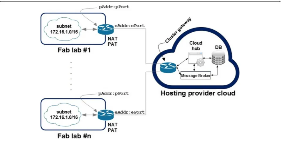
The NEWTON Fab Lab architecture is a three-tier spoke-hub architecture in which the interconnected Fab Labs (i.e. the spokes) can communicate through a cen-tralized hub located on cloud premises. The digital fabri-cation equipment of each Fab Lab is not directly exposed to the internet but can be accessed through a Fab Lab gateway that implement filtering and security policies. Finally, each digital fabrication machine has a software wrapper that exposes the underlying hardware though a set of REST APIs. Both the Fab Lab gateway and the machine wrapper are implemented using inex-pensive off-the-shelf microcontroller boards. In our specific case, we use Raspberry PIs boards to implement the gateway and the machine wrappers; for this reason, we also refer to them as Pi-Gateway and Pi-Wrapper re-spectively. Fig.1depicts the simplified architecture of the NEWTON Fab Lab infrastructure. In order to allow inter-Fab Lab communication, each networked inter-Fab Lab should have at least one public IP address _Addr:ePort. The router/gateway maps the inbound traffic into a private

address pAddr:pPort by means of a Network Address Table (NAT) and a Port Address Table (PAT). Similarly, the router performs the same task on the outbound traffic by forwarding it to the default gateway or by redirecting the requests for a private address to the private network. The message flow between the cloud application and the networked Fab Labs is managed by a cloud-deployed mes-sage broker that implements a publish/subscribe protocol. Spoke and hub nodes form a Virtual Private Net- work (VPN) in which the Fab lab gateway and the virtual machine instances on cloud premises communicate se-curely over the internet using private IP addresses though an IPSec (IP Secure) tunnel. IPsec is a suite of protocols for managing secure encrypted communications at the IP Packet Layer. The cloud and Fab Lab gateways are the tunnel endpoints deployed on local and cloud premises respectively.

The cloud hub

The Cloud Hub is the centralized communication hub for all the networked NEWTON Fab Labs, tightly inte-grated into AWS (Amazon Web Services) web services infrastructure. More specifically, the cloud hub infra-structure requires the following AWS managed services:

1. Route 53as the Domain Name Service (DNS). 2. S3as the backend storage for the application

cluster.

3. Internet Gatewayto expose to the internet the underlying public infrastructure.

(4)

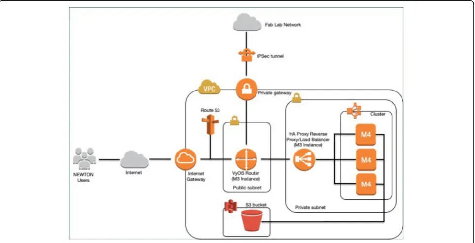
Figure 2 depicts the minimum infrastructure require-ments for the cloud hub. The deployment requires five EC2 (Elastic Compute Cloud) instances. Two m3.medium instances are necessary to deploy the service networking infrastructure, whereas, three m4.large instances are ne-cessary to deploy the cluster with the Platform as a Service Infrastructure (PaaS) to manage the Fab Lab cloud services. Digital fabrication services (i.e. the fabrication machines software wrappers and the underlying hard-ware) can be accessed through a set of REST APIs described in [10]. The cloud service networking infrastruc-ture is formed by:

– A VyOS4software-defined router to forward the incoming traffic from both the internet gateway and the IPSec tunnel to the service cluster in the private sub-network.

– A reverse proxy to route the traffic forwarded by the VyOS router to the target service running on the service cluster.

The VyOS router is also used to manage the cloud end of the IPSec tunnel that connects the cloud hub to the Fab Labs network. Thus, the cloud hub and the in-terconnected Fab Labs form a unique VPN in which cloud and on- premise services communicate over an encrypted channel using private IPs.

The PaaS infrastructure is deployed on top of Flynn.5 Flynn can be considered as a grid of Docker containers, ra-ther than a traditional cluster. Each host will run container-ized services and applications that can be deployed and scaled individually. Fig.3shows a simplified diagram depict-ing a Flynn grid deployment across a cluster of three hosts. Flynn architecture is split into two layers.Layer 0provides basic services such as host management, service discovery and scheduling, whereaslayer 1implements the PaaS busi-ness logic (GitHub interface, Slug Builder, Slug Runner, etc.). Referring to Fig.2, the layer 0 services are:

1. The Host Service (HS) that implements the interface between Flynn services and Docker. The Host Service is the only one that must run across all the Flynn hosts 2. The Scheduler (S). The scheduler distributes the

containers among the instances given the current state of the grid and the resource allocation in each node.

The layer 1 services are:

1. The GitHub frontend (G). This module accepts Git connections through SSH and Git pushes; then deploys them in the Flynn grid.

2. The Controller (C) exposes APIs to control the whole infrastructure.

3. The Router (R) is a TCP/HTPP router/load balancer that distributes the incoming requests through the instances deployed in the Flynn grid. In order to implement a high-availability there must be several instances of this module across all the Flynn hosts.

4. The Slug Builder (SB) is a module that builds a slug starting from a Git push received by the Flynn Git front-end (G). A slug is a compressed and pre-packaged copy of an application optimized for distribution to the Flynn PaaS.

5. The Slug Runner (SR) is a module that allocates and instantiates several Docker containers (depending on the scaling parameters) to deploy and execute the code contained in a slug. 6. The Application (A) is a module that

implements the application code (for example, the Cloud Hub and the Service Registry in our specific case).

The fab lab gateway

The Fab Lab gateway (i.e. the Pi-Gateway) is the entry point to the local network and to the digital fabrication in-frastructure of a Fab Lab. Fig. 4 depicts the Pi-Gateway software architecture. The architecture is modular and distributed over four layers. The Communication Layer is a proxy server that implements the communication proto-cols between the cloud hub and the gateway (HTTP and HTTPS are both supported). The incoming requests are forwarded to the API Wrapper Layer that implements simple APIs to communicate with the underlying Fab Lab infrastructures and a simple reactive websocket proto-col to update in real-time the Fab Lab status in the cloud hub infrastructure. The proxy configuration is managed by a command line interface (CLI). Both the CLI and the API wrapper layer leverage the Middle- ware Layer func-tions to implement the business logic and the communi-cation protocols. Middleware provides primitive functions to implement websocket communications, logging, process management (using programmatically the APIs provided by the PM26module), transactional e-mail (using an AWS Simple E-mail Service client) and persistence layer interfacing. Open API 2.0 (Swagger) support is also integrated in the middleware layer and APIs specifi- cat-ions are described in [11]. Finally, the Data Layer (persist-ence layer) is used to store the proxy and the Fab Lab configurations. We use a NoSQL model and Redis7 mod-ule) as the key-value store.

4_{https://vyos.io} 5_{https://flynn.io}

(5)

The machine wrapper

The Machine Wrapper (i.e. the Pi-Wrapper) provides the connected machine with a software abstraction layer by exposing the machine functionalities through a set of APIs. Fig. 5depicts the software architecture of the Pi- Wrapper. The software architecture is modular and distributed over five layers. The Communication Layer implements the HTTP server and the APIs interface to manage and schedule fabrication batches. The Presentation Layer implements the user interfaces to set up and manage a connected fabrication machine. An MVC (Model View Controller) programming paradigm is used at this stage; namely, a route in the browser triggers a controller function that dynamically generates and renders an HTML view using the data stored in the persist-ence layer (i.e. data base). The Application Layer implements the business logic. The business logic and the user interface rely on the middleware functions implemented in the Middleware Layer. More specifically, the middleware in-cludes custom and third-party methods to manage security and authentication, machine to machine communications and interfacing, HTML views rendering, system logging, data base connection and access, and ADC (Analog to Digital Converter) drivers to sample data from the machine moni-toring circuit as described in [9]. Open API 2.0 (Swagger) support is integrated in the application middleware, this makes the Pi-Wrapper a very developer- friendly software since APIs and data models documentation is embedded into the application, in addition a developer can test the API using the Swagger User Interface that is also embedded in the Pi-Wrapper. Swagger Pi-Wrapper API specifications are described in [12]. Finally, the Data Layer is used to store ses-sion information as well as User and Machine data models. We use a NoSQL model and MongoDB8

as the data store.

Machine to machine communication

The communications between client applications and the remote NEWTON Fab Labs rely on a protocol stack which includes a simple publish/subscribe protocol. The fabrication equipment is accessed through the Fab Lab Gate- way that routes incoming commands to a given machine depending on both availability and the specific task to be carried on. The communication protocol re-lies on a server-to-server model in which some nodes act as message brokers collecting the incoming messages and re- laying them towards a destination node. A fabri-cation job is routed to a networked Fab Lab by the Cloud Hub message broker; however, the message bro-ker on the cloud side has not direct visibility of the Fab Lab network infrastructure. Its main task is to connect a client to the Fab Lab infrastructure or to perform inter-Fab Labs message routing. The networked machines in a Fab Lab can be accessed through the Fab Lab Gateway

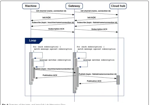
only. The gateway main task is routing the outbound traffic to the networked equipment and managing intra-Fab Lab communications. Fig. 6 presents a simplified timing diagram that describes the communication be-tween the cloud infrastructure and a networked Fab Lab. The message exchange has four stages:

1. link establishment; 2. topic subscription; 3. communication;

4. disconnection (not illustrated for the sake of simplicity).

Once the TCP links between the machine and the Fab Lab Gateway on one side, and the Fab Lab Gateway and the Cloud hub broker on the other side, have been established, both the Gateway and the Hub subscribe to topics they are interested in. The topic string is generated using the unique name and connection ID sent by the server that initiates the communications to the destination server during the link es-tablishment. Both the link establishment and the subscrip-tion phases are terminated by an ACK message (Init ACK for the link establishment and Subscription ACK for the subscription phase). In other word, the Fab Lab Gateway and the Cloud Hub implement a double broker architecture: the former collects all the incoming messages from the Fab Lab machines whereas the latter collects all the incoming messages from the networked Fab Lab Gateways. The double broker architecture allows the implementation of Fab Lab access and security policies and of custom mes-sage filters mechanisms. Once the subscription phase has terminated, the end nodes start exchanging messages. Each published message can be acknowledged by an optional Publication ACK message. The use of a Publication ACK is mandatory in those cases when it is necessary to guarantee the delivery of a message and to implement retransmission mechanisms to increase the QoS of the protocol.

Test, modelling and simulation

The system infrastructure has been tested in real scenar-ios through small-scale pilots that have involved the par-ticipation of six schools and universities located in three European countries as part of the EU-funded NEWTON project. The test pilots have been used to stress the system infrastructure and evaluate the per-formance of the proposed algorithms for task scheduling and fabrication resources allocation. In order to detect system peak performance, system infrastructure and APIs have been also load tested using Locust.9 Locust allows to simulate user behavior using a Python script. We have designed a set of simple use cases that stresses

(6)

all the Fab Lab APIs and provides a unified picture of the system performances.

The test scenario implements the use cases de-scribed in Table 1. These use cases have been trans-lated into a Python script that is parsed by Locust in order to generate the requests for the infrastructure under test. Locust can be further configured so that the user behaviour described in that script can be as-sociated to an arbitrary number of virtual users in order to stress the system response under different load conditions.

Load tests

The Fab Lab infrastructure described in the previous sections has been load tested in the following emulated scenarios:

1. 50 concurrent users with a hatch rate of 5 users per second.

All the incoming requests are forwarded to the same fabrication machine, each test has a duration of 2 mi-nutes and, as mentioned before, each simulated user performs the operations described in Table 1 which means that the following HTTP requests are sent to the Fab Lab APIs:

1. GET the available Fab Lab status. 2. POST a job to the available Fab Lab.

3. GET the status information of the submitted job.

(7)

4. DELETE the submitted job.

5. GET the information of the jobs running in the available Fab Lab.

The most time-consuming operation is the POST re-quest to submit a fabrication job since it involves the fol-lowing steps:

1. Uploading the image on the cloud hub. 2. Sending the image to the Fab Lab Gateway. 3. Sending the image to the target fabrication

machine.

4. Update the jobs queue in the fabrication machine.

Fig7shows the load tests results for the three scenar-ios under test (i.e., the cases with 50, 100 and 150

concurrent users respectively). Fig. 7 a summarizes the overall results for all the request types, whereas Fig. 7b depicts the results only for POST requests. Test results are excellent, considering the Fab Lab infrastructure has been deployed on inexpensive Raspberry Pi III boards. For example, the 90% of the incoming requests are served in maximum 680 ms for 50-user scenario, 1100 ms for the 100-user scenario, and 5100 ms for 150-user scenario. Of course, as outlined earlier in this section, the most time-consuming operations are the POST re-quests whose delay can be as high as 9141 ms in the case of 150 concurrent users. An overview of the measure-ments performed using Locust is summarized in Tables

2, 3 and 4. The tables report the median, minimum, maximum and average response time in milliseconds for each one of the API called by our simulated scenario for

(8)

all the test cases studied (namely for the 50-, 100- and 150-user load respectively). The measured values con-firm the excellent performance already outlined by Fig.

6. The total average response times for the 50-, 100- and 150-user test cases are 452 ms, 568 ms and 1680 ms re-spectively, whereas the maximum average response times are 801 ms, 1158 ms and 3883 ms respectively. An average response time of 3883 ms is acceptable and, ac-cording to Fig. 7 a allows, on the average, the comple-tion of the 100% of the requests for the 50-user scenario, the 99% of the requests for the 100-user scenario and

almost the 80% of the total requests for the 150-user scenario.

Platform modelling

The system stressed by the load tests described in Sec-tion 3.1 is a minimum deployment formed by the Cloud Hub located in theeu-central-1AWS region (i.e., in the Amazon AWS data center in Frankfurt) and a single spoke node (i.e., the San Pablo-CEU Fab Lab located in Madrid). Thus, in order to estimate the performances of

Table 1Fab Lab modules test cases

Id Test case objective Test case description Expected result

1 Check the interface link between the

REST client and the Cloud Hub

Authenticate with the JWT token The user is authorized and can use submission APIs

2 Check the interface link between the

Cloud Hub and the Fab Lab Gate- way

Send a request to the Fab Lab gateway

The user submits a job, the request is forwarded to the Fab Lab gateway and the all the data bases are correctly updated

3 Check that a fabrication batch is

successfully delivered to a machine

Send the request to the machine wrapper

The gateway forwards the requests to the wrapper and all the databases are correctly updated

4 Check that the system correctly stores

all the fabrication requests

The user gets a list of the jobs he/ she has submitted to fabrication

The user receives a response with the list of the submitted jobs and the fab lab details

5 Check that a fabrication batch can be

cancelled

The user cancels a fabrication batch The cancellation request is delivered to the machine, the job is cancelled and all the databases are correctly updated

(9)

larger deployments across several AWS regions, a simu-lation model is necessary. The cloud infrastructure under test, depicted in Fig. 8, is very complex and re-quires up to six levels of AWS services (Route 53, Elastic Load Balancing, Autoscaling, EC2 instances, S3 storage and optionally, Cloudfront CDN services). This, in turn entails several challenges tied to infrastructure and appli-cation setup, administration, and behaviour predictabil-ity. On one hand, the promise of scalability, redundancy and on-demand service deployment makes a cloud im-plementation a very appealing solution. On the other hand, all these advantages come at the price of several issues that can make cloud application development and management a challenging task. More specifically, the is-sues with cloud deployment are related to the following impact factors:

– Performance:Disk IO operations can be a serious issue and limit the performance of a cloud deployment. In a cloud infrastructure, the network and the underlying storage are shared among customers. If, for example, another customer sends large amounts of write requests to the cloud stor-age system, your application may experience slowdowns and its latency becomes unpredictable. Moreover, also the upstream network is shared among customer, so one can experience bottlenecks

there too. Unluckily, cloud vendors use to offer to their customers large storage, but not fast storage.

– Transparency:Transparency and simplicity are key factors when debug- ging either an application or an infrastructure. Unfortunately, cloud services are, in many cases very opaque and tend to hide underlying hardware and network problems. Cloud infrastructure is a shared service, and, for this reason, cloud users may experience issues that do not occur in dedi-cated infrastructure. More specifically, cloud infrastructure customers, share hardware

resources such as CPU, RAM, disk and network, thus the workload of other users can saturate a computing node and heavily affect the

performance of your application.

– Complexity and scalability:Fig.8gives an idea of the complexity of the cloud architecture that has been deployed to ensure NEWTON Fab Labs connectivity. This entails the interaction of up to six different AWS service layers that require expertise for set-up and configuration. Moreover, Elastic Load Balancing and scalability are not straightforward in AWS and require the deployment and configuration of additional services (namely, CloudWatch and CloudFormation) that incur extra costs and complexity.

Fig. 7Percentage of Requests Completed in a Given Time IntervalaTotal Requests, andbPOST Requests

Table 2Summary of System Performance for 50 Users Load (values are in ms)

API call Median min 50 users avg.

max

GET /fablabs 220 137 2990 313

GET /fablabs/fablab:id/jobs?job = job:id 205 139 664 246

DELETE /fablabs/fablab:id/jobs?job = job:id 438 285 3508 546

GET /fablabs/jobs 210 139 3370 354

(10)

Finally, as mentioned in Section 2.1, we have deployed a PaaS (Platform as a Service) infrastructure on top of the cloud infrastructure depicted in Fig8. The PaaS simplifies application and service deployment in a cloud environ-ment but adds other software layers and additional com-plexity to the underlying infrastructure, making the application behaviour even more unpredictable. In order to build a simulation model as close as possible to the real behaviour of the cloud infrastructure, we have followed the steps reported in the sequel:

1. We have instrumented the Cloud Hub server in order to measure the server latency to process an incoming request.

2. We have developed a fake client that performs fabrication requests at random times and have measured the elapsed times from request arrival to request dispatch to the selected Fab Lab. This time represents the server latency that is necessary to serve a request.

3. We have performed latency measurements for several server configurations, scaling the number of containers allocated to the database and to the Cloud Hub application.

4. We have used the measured data to build a simple regression model to predict the server latency as a function of the incoming requests and of the number of allocated containers.

5. We have deployed a test infrastructure across several AWS data centers in order to ensure the maximum geographic coverage as depicted in Fig.8. The Fab Lab network implements a spoke-hub architecture in which each spoke relies on the Registry Server of the Cloud Hub for service detection and trac routing. 6. We have performed several measurements on the cloud infrastructure in order to determine latency and bandwidth across the networked Data Cen- ters. 7. We have used RIPE Atlas10data to build a latency

and bandwidth model for the connections among a client and a Data Center and a Data Cen- ter and

the target Fab Lab for each geographic region covered by AWS infrastructure.

8. We have used the experimental data gathered in Steps (6, 7) and the simple predictive model developed in Step (4) to build a delay model for the NEWTON Fab Lab infrastructure.

9. We have built an ad-hoc simulator on top of CloudSim [13] to simulate the behavior and the performance of the NEWTON Fab Labs network under different load conditions and using the delay model implemented at step (8).

Cloud hub delay estimation

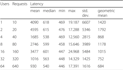
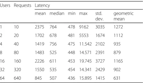
The Cloud hub server has been instrumented in order to capture the the incoming POST requests and to meas-ure the time elapsed from the request arrival and its sub-sequent forwarding to the selected Fab Lab. The measurements have been performed for several request-ing users and server configurations. For each simulation set up the measurements have been performed 10 times at random intervals. We assume that the number n of requesting users is a power of 2 with 1≤n≤64 and that the number c of Docker containers allocated to the Cloud hub server is also a power of 2 with 1 ≤ c ≤ 8. For each configuration under test we compute the mean, the median, the standard deviation and the geometric mean of the measured latencies. The measurements are reported in Tables 5, 6, 7 and 8. Tables 5, 6, 7 and 8

summarize the statistical distributions of the measured delays for several application deployments. As also ob-served in [9], the measured values exhibit a high stand-ard deviation. Moreover, observing the minimum, the median and the maximum values, one can infer that the measured latencies have a tail distribution (either log-normal or Pareto). This tail behaviour, as reported in [14], is typical for networked and internet applications. More specifically, we have found that the distribution of the measured values, whose statistical behaviour is sum-marized in Tables5,6,7and 8, matches a Pareto type I distribution.11 Due to the high dispersion of the

10_{https://atlas.ripe.net}

11_{The experimental data has been open-sourced and is available at}

https://github.com/gcornetta/data

Table 3Summary of system performance for 100 Users Load

(values are in ms)

API call median min 100 users avg.

max

GET /fablabs 220 137 3515 347

POST /fablabs/jobs?machine = type&lat =..

. 830 398 5233 1158

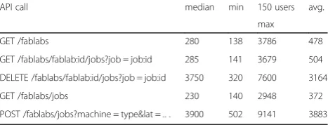
Table 4Summary of System Performance for 150 Users Load

(values are in ms)

API call median min 150 users avg.

max

GET /fablabs 280 138 3786 478

(11)

measured data, the mean values are not meaningful and may lead to wrong conclusions since the arithmetic mean is heavily affected by the outliers. A more objec-tive analysis must rely on the minimum and median values of the latency as well as on its geometric mean since, unlike arithmetic mean, it is less sensitive to the effect of the outliers. Analyzing Tables5, 6,7and 8as a whole, one could easily observe that the minimum, the median and the geometric mean of the measured delays

decrease as expected (with some outliers) as the number of allocated containers scales up. However, this is not the case for the maximum delays. As mentioned before, Downey [14] showed that this high variability is very typical in internet applications. In our specific case, the high dispersion of the measured values is due to the un-predictable latency introduced by the cloud infrastruc-ture. As pinpointed in Section 3.2, a cloud deployment has some drawbacks that arise from the fact that several

Fig. 8NEWTON Fab Labs global infrastructure deployment

Table 5Cloud Hub latency (in ms) with one container allocated

to the application

Users Requests Latency

mean median min max std.

dev.

geometric mean

1 10 1815 1307 513 4294 1307 1424

2 20 1935 1448 525 5132 1560 1418

4 40 1636 1122 516 5298 1388 1238

8 80 1592 984 477 5280 1386 1189

16 160 1368 871 474 6636 1184 1048

32 320 1302 898 473 6654 1073 1034

64 640 1273 936 458 5742 881 1052

Table 6Cloud Hub latency (in ms) with two containers

allocated to the application

dev.

geometric mean

1 10 4090 618 469 19.187 6607 1420

2 20 4595 615 476 17.288 5346 1792

4 40 1685 538 469 12.560 2815 868

8 80 2746 599 458 15.646 3989 1178

16 160 3477 601 447 24.968 5484 1015

32 320 1016 563 448 14.329 1425 752

(12)

customers are sharing the same virtualized hardware and network infrastructure. Consequently, the perform-ance of a cloud application is heavily affected by the other customers’application that are loading the under-lying infrastructure at the same time. We have deliber-ately performed our measurements at random times to trigger this variable behavior and the effect of the other AWS customers application load on the performance of our platform. To this latency, we should also add the la-tency introduced by the virtual networking routing infra-structure deployed by Flynn. However, recall that the impact of the maximum delay on the overall perform-ance is minimum; since, in a tail distribution the prob-ability of a high delay is very low.

Communication latency and bandwidth

In order to build a realistic simulation model, we need to estimate communication latency and band-width among the nodes that form the Fab Lab net-work as well as the maximum concurrency level that each node can support. This goal is accomplished through the following steps:

– We estimate the network latencyLcjfrom client to

Data centerjandLfjFab Lab to Data Centerjin the

same AWS region. To do this, we use the real measurements provided by RIPE Atlas network. RIPE Atlas is a public network located in the last mile and formed by more than 16.000 measurement probes capable of measuring connectivity between internet endpoints on demand.

– We estimate the network uplink and downlink bandwidth between client and Data Centerj

(Buplink,cjandBdownlink,cjrespectively) and Fab Lab

and Data Centerj(Buplink,fjandBdownlink,fj

respectively) in the same AWS region. To do this, we use the Clouharmony speed test service.12 How-ever, this service allows measuring the desired

parameters only between the client browser and the target Data Center. This means, that we are able to track performance only within Europe and must make the simplifying assumption that the network

performances within the same AWS region are approximately the same using the measurements performed in Europe as the reference values.

– We measure the Data centerito Data centerjnetwork latency_Lijusing ping and traceroute. Traceroute is even

better than ping since it allows testing the response time of each network segment along the path. There-fore, this tool can not only measure but also locate the latency across the routers that form the packets path.

– We measure the Data centerito Data centerj

uplink and downlink band- with (Buplink,ijand

Bdownlink,ijrespectively) using iPerf3 tool.

The delayDof the system response after a fabrication (POST) request has been issued is computed as follows:

D ¼ Lcjþ tuplink;cj þ Ljk þ tuplink;jk þ Lkj þ tuplink;kj

þ Ljf þ tuplink;cj þ Lfj þtuplink;fj þ Ljc þ tuplink;jc ð1Þ

where j denotes a Datacenter located in a spoke node, whereas k denotes the Data center located in the hub

node. The delay D of a response is hence the packet

round-trip time necessary to follow the path the goes from the client to the spoke node, from the spoke to the hub node and then to the spoke again, from the spoke to the selected fab lab and then to the spoke again, and finally to the client. Observe that the data transfer time tijbetween nodesiandjin Equation1is computed as:

tij ¼ Sij

Bij ð2Þ

where Sij and Bij represent, respectively, the number of

bytes transmitted and the measured bandwidth between 12_{https://cloudharmony.com/speedtest}

Table 7Cloud Hub latency (in ms) with four containers

dev.

geometric mean

1 10 798 501 477 2660 757 644

2 20 1418 527 477 7521 2016 816

4 40 1852 549 478 12.302 2731 1002

8 80 2260 608 443 12.944 3100 1153

16 160 2613 698 465 12.944 3500 1251

32 320 1750 509 446 12.069 2566 907

64 640 1190 508 447 14.704 2081 710

Table 8Cloud Hub latency (in ms) with eight containers

dev.

geometric mean

1 10 2375 764 478 9162 3035 1272

2 20 1702 678 481 5553 1674 1112

4 40 1419 756 475 11.542 2102 935

8 80 1483 525 448 14.571 2391 879

16 160 2226 611 453 19.745 3727 1165

32 320 1550 535 454 14.341 2429 902

(13)

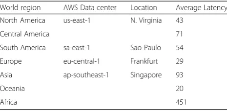
nodesi and j. Table9 summarizes the average latencies measured from client to Data center from different world regions.

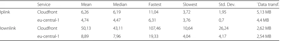
Table10reports the uplink and downlink bandwidth be-tween a client and a Data center located in the same AWS region. More specifically, these measurements refer to a client and a Data center located in Europe since, as we pointed out earlier, the Cloudharmony speed test service only allows performing measurements from the client browser to the target Data center. We will use the values of Table9as reference for all the AWS supported region that form the NEWTON Fab Lab network architecture.

Table11reports the Data-center-to-Data-center latency. For each possible connection, we report minimum, aver-age and maximum latency as well as the standard devi-ation with respect the average latency.

Finally, Table12summarizes the measured uplink and downlink bandwidths for the Data center to Data cen-ter connections.

Concurrency level

We use Apache Benchmark13 to estimate the maximum concurrency level that can be effectively borne by a node of the NEWTON cloud infrastructure. This allows us to esti-mate the maximum number of concurrent requests that can be served by the cloud infrastructure and to configure suit-ably the simulator that models NEWTON Fab Lab infra-structure. The Cloud Hub APIs provide a root (/) endpoint that supports both HTTP and HTTPS protocols and returns a response with a 200-status code and a body with an empty JSON (JavaScript Object Notation) object. We use this end-point to ping the Cloud Hub sever; however, we can also use the same endpoint to perform simple load tests on our infrastructure. Nonetheless, you have to keep in mind that the result obtained in this way are optimistic since the au-thentication server and the underlying data base are not stressed. Although Apache Benchmark tool generates very detailed reports, we are only interested in detecting which is the maximum number of concurrent requests that breaks our server leading to a timeout error. In order to do this, we stress our server during a prolonged period with an increas-ing number of concurrent requests until it breaks. Table13

summarizes the percentiles measured when a minimum cloud deployment (with only one container allocated to the cloud hub application) is stressed by 20.000 requests with concurrency levels 10, 50 and 100 respectively. Observing the percentiles of the measurements, we note that in all the scenarios under test the response delays exhibit a tail distri-bution. In addition, increasing the concurrency level of the incoming requests leads to larger tail delays, being 100 the maximum concurrency level that can be supported by the cloud configuration under test. However, the measurements

carried out are qualitative and are only useful to set-up our simulation model with reasonable values. In fact, the mea-surements performed have been carried out just for a short period of time, thus they do not consider the delay variabil-ity of the cloud infrastructure as pointed out previously. Moreover, the measured times refer to the response latency for a simple API endpoint that returns a 200-OK response; consequently, they do not consider the extra latency to ac-cess to the underlying data base to retrieve the Fab Lab in-formation. For all the aforementioned reasons, it seems reasonable to assume that, in a real deployment, the Fab Lab infrastructure can support without problems up to 50 concurrent accesses and manage approximately 1000 re-quests per second (by scaling up the number of containers allocated to the cloud application).

Simulator implementation and simulation results

The measurements performed on the Cloud Hub infra-structure reported in Tables 5 to 8 show, as expected, non-normal distribution of the measured data that seems loosely correlated to the number of requests and the number of containers allocated to the application, which makes very difficult to make reliable predictions of the Cloud Hub ap-plication latency. Lognormal and Pareto distributions are those that better model server response time [14]. For this reason, the proposed prediction scheme does not predict the latency of the Cloud Hub application; this would make no sense, since, as stated before in a cloud environment several customers share the same network and infrastruc-ture which makes very hard to predict the server behaviour in a given instant. What we do instead, is using the mea-sured data to predict the shape of a type

I Pareto distribution that models the performance of our cloud infrastructure under different load conditions and number of allocated containers. We then use the prediction to generate, in our simulator, a random la-tency X(r, n) that is a function of the number r of in-coming requests and of the number n of allocated containers, with that Pareto distribution starting from a

Table 9Summary of the latencies (in ms) of client-to-Data

center connection

World region AWS Data center Location Average Latency

North America us-east-1 N. Virginia 43

Central America 71

South America sa-east-1 Sao Paulo 54

Europe eu-central-1 Frankfurt 29

Asia ap-southeast-1 Singapore 93

Oceania 20

Africa 451

(14)

uniform random variable U ∈(0, 1) using the following equation:

X rð ;nÞ ¼ ^xiðr;nÞ 1−U

ð Þ1=^αð Þr;n ð3Þ

Where βˆ(_{r, n}) =_xˆi(_{r, n}) is the prediction of the Pareto distribution scaleparameter and αˆ(r, n) is the prediction of the Pareto distribution shape parameter. Bothβˆandαˆ are computed using a simple regression model as a func-tion of rand n. The simulation software has been built according to the following hypothesis:

1. The CPU load of each instance of the cluster must not exceed the 50%.

2. The requests are evenly distributed among the cluster instances.

3. The incoming requests are evenly distributed within a given instance among blocks of 8 Docker

containers, being 64 the scaling threshold.14 4. The cluster minimum configuration can manage up

to 50 concurrent accesses.

The following pseudo-code snippet describes the block allocation and latency estimation process implemented by our simulator:

The algorithm estimates the delay of the infrastructure response and follows the steps described next. First an

array to hold the estimations of the response delay is ini-tialized (line 1). Afterwards, the number of incoming re-quests is computed and the number of containers necessary to manage all the incoming requests is allo-cated in each of the virtual machines that form the clus-ter (lines 3 to 7). Then, the number of requests that must be forwarded to each allocated block of containers is computed (line 8). After that, for each allocated block, the shape of the Pareto distribution of the possible de-lays is computed (lines 9 to 13). Recall that, as stated be-fore, the Pareto distribution shape and scale parameters are computed by performing a multivariate linear regres-sion on the measured data whose statistics are summa-rized in Tables 5, 6, 7 and 8. Finally, the values of the shape and scale parameters for the given number of re-quests and allocated containers are used to estimate the system response latency using Equation3.

Thus, our simulator relies on the measurements re-ported in Sections 3.3 to 3.5 to build a network band-width and latency model and on Equation3 to estimate the delay of the spoke and hub nodes taking into ac-count the variability introduced by the cloud shared in-frastructure. The overall system delay, i.e. the packet round-trip time from a fabrication request issued by a client until the system acknowledge is computed using Equation 1. Experiments have been designed to analyze the behaviour of the NEWTON Fab Lab infrastructure with the following users’ distribution: 250, 500, 1000, and 1500. Each user can issue from one to five requests; moreover, for each load configuration, the number of containers allocated to the application will scale as mul-tiples of 8 from 8 to 128 (for 16 possible configurations). Finally, the simulated infrastructure must cover requests from four AWS availability zones (Europe, North and Central America, South America and Asia-Pacific) in order to ensure a globally optimal service to all the world regions. Table 14 summarizes the experiments configurations. The variable simulation parameters are the number of users, the number of requests per user,

14

This design choice is due to the fact that our simple prediction functions are defined for 1≤r≤64 requests and 1≤n≤8 containers. Also, consider that Flynn does not natively support the container autoscaling feature implemented by our simulator. In order to enable container autoscaling you should use other container orchestration platforms such as DC/OS or Rancher instead of Flynn, provided you may afford higher deployment costs.

Table 10AWS uplink and downlink bandwidths (Mb/s)

Service Mean Median Fastest Slowest Std. Dev. `Data transf.

Uplink Cloudfront 6,26 6,19 11,04 3,72 1,95 5,13 MB

eu-central-1 4,74 4,47 6,31 3,76 0,7 4,4 MB

Downlink Cloudfront 50,13 43,11 107,46 10,64 26,24 2,62 MB

eu-central-1 8,89 7,96 19,33 4,04 4,17 2,54 MB

Table 11Summary of the hub-to-spoke latencies (ms)

Connection minimum average maximum std. dev.

eu-central-1 - us-east-1 87,95 88,121 88,958 0,377

eu-central-1 - sa-east-1 226,968 227,837 233,604 1634

(15)

and the number of containers allocated to each in-stance of the cluster. All the other parameters are fixed. This means that for each possible user config-uration 80 experiments must be performed (i.e. the number of requests per user times the number of possible containers configurations). For the sake of simplicity, we also assume a uniform user distribution among different AWS regions.

The scaling threshold is set to 1024 requests, i.e. the request count per target of each Elastic Load Balancing (ELB) target group must be kept as close as 1024 for the Autoscaling group.15More specifically, assume that you have configured an Autoscaling group with a minimum of three instances (i.e. the minimum PaaS cluster config-uration) and a maximum of six instances within an ELB group of a given AWS region. Setting a threshold of 1024 means that each instance of your cluster should re-ceive approximately 1024 requests. If the overall number of incoming requests is larger, the number of instances should be scaled up to match the target threshold as close as possible. For example, if the cluster has three in-stances and the number of incoming requests is, say 3800, the system should scale up by one instance (i.e. from three to four), so that each instance handles 3800/ 4 = 950 requests. Finally, note that with the simulation set up depicted in Table 14, the maximum number of incoming requests from a given region do not exceed

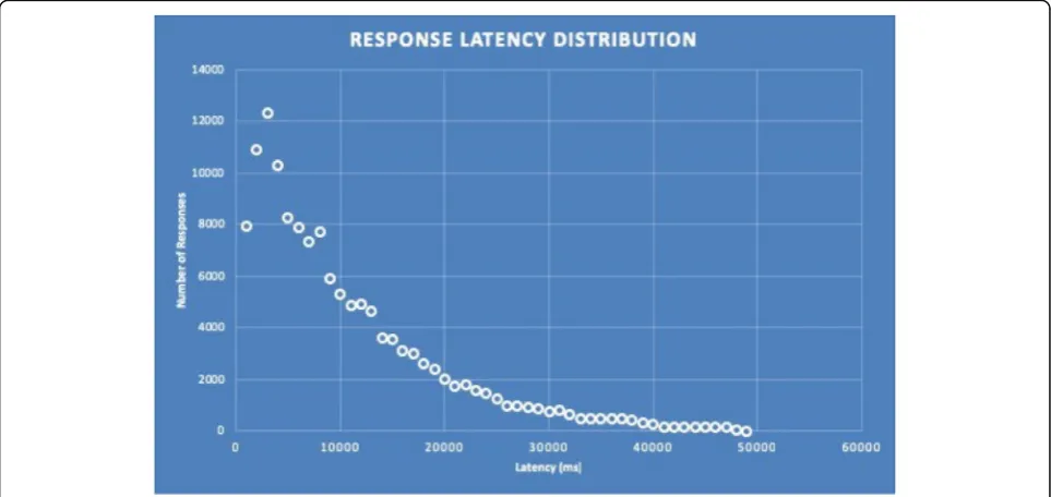
5000; thus, with a threshold of 1024 it is not necessary to have more than five virtual machines in the Autoscal-ing group. Prior to runnAutoscal-ing all the experiments, we have to make sure that the mathematical model we have de-veloped for the cloud application behaves as expected. To do this we simply check that the simulated latency of the NEWTON cloud infrastructure matches a Pareto distribution. After running all the simulations whose set-up is detailed in Table14we obtain the Pareto-like dis-tribution of the response latency depicted in Fig. 9. Re-call that, as detailed in Table14, our simulation scenario assumes fabrication requests with a 5 MB attachment (since this is the typical image le size of a design submit-ted for fabrication). In addition, we have also assumed that the users (and hence the service requests) are evenly distributed among all the Data centers that form the NEWTON Fab Lab cloud infrastructure.

Table15represents the percentiles for the distribution of Fig. 9. Observe that 50% of the requests are served within 8000 ms and 99% of the requests within 38.000 ms, being 49.000 ms the worst-case simulated delay. These are indeed excellent results considering that:

– As highlighted earlier in this paper, cloud infrastructure is shared among many customers, leading to very variable delays.

– The simulated latency also includes the transmission time of the design le (assumed to be 5 MB) attached to a request (that must go from the client to the spoke or hub node of NEWTON infrastructure and finally to the target Fab Lab).

– In the worst-case scenario the communication delay depends on the following path: client - spoke - hub - spoke - Fab Lab - spoke - client. Thus, the latency of a response can be very high due to the

communication overhead introduced by each node in the communication path.

15

Please note that in a real (i.e. not simulated) AWS deployment you need to enable the CloudWatch service to measure the metrics necessary to trigger autoscaling and the CloudFormation service to create and deploy an instance of the PaaS cluster node.

Table 12Summary of the Inter-Data center uplink and

downlink bandwidths (Mb/s)

Connection minimum average maximum std. dev.

Uplink eu-central-1 -

us-east-1

17,4 37,59 69,80 18,35

eu-central-1 - sa-east-1

7,39 18,88 35,5 8,58

eu-central-1 - ap-southeast-1

3,57 5,91 8,07 1,74

central-1 - eu-central-1

21,9 82,89 188 49,2

Downlink eu-central-1 - us-east-1

15,8 35,23 67,1 18,19

eu-central-1 - sa-east-1

6,71 15,82 33,4 8,45

eu-central-1 - ap-southeast-1

3,34 5,67 7,89 1,76

central-1 - eu-central-1

20,4 80,73 185 48,72

Table 13Summary of the response times (in ms) for 20.000

incoming requests

Percentile Concurrency level

10 reqs. 50 reqs. 100 reqs.

50% 45 44 46

66% 46 45 48

75% 46 47 49

80% 47 48 51

90% 49 51 57

95% 64 60 64

98% 74 70 71

99% 80 74 85

(16)

After running the set of experiments described in in Table 14, for each Data center in the network, we ob-tain the performance estimations summarized from Table 16, 17, 18, 19, 20 and 21. For each simulation scenario and Data center, we report minimum, max-imum, average, median and standard deviation of the simulated latency.

Observing the simulation results we can easily infer that the cloud system infrastructure behaves as expected since:

1. The response delay increases with the number of requests.

2. The Europe Data center is the one that exhibits the longest delays because it is the hub of our

infrastructure and must always process all the incoming requests.

3. The Data center latency exhibits a high variability, which reflects the performance fluctuations of the cloud infrastructure due to resource and network sharing with other customers as outlined

previously.

4. The response latency exhibits a Pareto-like distribution, which is typical of internet networked systems.

Infrastructure costs

The NEWTON infrastructure must comprise four Data Centers to ensure maximum coverage in all the AWS supported regions. The Data Centers im-plement a spoke-hub architecture being the

Frank-furt node (eu-central-1 AWS region) the hub.

Spokes must be located in United States (eu-east-1

Table 14Experiments conguration

Num. of users Reqs. per user Scaling threshold AWS zones Data transfer Virtual machines Num. of containers Num. of experiments

250 1 to 5 1024 4 5 MB 3 to 5 8 to 128 80

500 1 to 5 1024 4 5 MB 3 to 5 8 to 128 80

750 1 to 5 1024 4 5 MB 3 to 5 8 to 128 80

1000 1 to 5 1024 4 5 MB 3 to 5 8 to 128 80

1250 1 to 5 1024 4 5 MB 3 to 5 8 to 128 80

1500 1 to 5 1024 4 5 MB 3 to 5 8 to 128 80

Total: 480

(17)

AWS region), South America (sa-east-1 AWS region) and Singapore (ap-southeast-1 AWS region). The main infrastructure and application (i.e. the registry service, the Fab Lab monitoring service, the Fab Lab connection/routing service) is hosted on the hub, whereas the spokes only run a simple client to query the service registry and the router. With this ap-proach we limit the more expensive virtual ma-chines (i.e. the m4.large instances) to the network hub, whereas the spokes may rely on cheaper virtual machines (i.e. t2.micro instances).

In its minimum configuration, the NEWTON cloud infrastructure relies on the following Amazon AWS services:

– Between five and eight Elastic Cloud Computing (EC2) instances.

– Between five and eight EBS volumes allocated for each EC2 instance.

– Route53 DNS service.

– S3 storage to implement the blobstore for the PaaS infrastructure.

Table 15Percentile table of the simulated NEWTON Fab Lab

cloud infrastructure latency

Percentile Latency (in ms)

50% 8000

75% 13.000

95% 26.000

98% 33.000

99% 38.000

100% 49.000

Table 16Summary of the Data centers performance (250 users

scenario)

250 users scenario

Reqs. per user

Data center Latency (ms)

min max avg. median std. dev.

1 North America 1180,232 2166,382 1536,937 1492,192 260,5785

South America 1480,398 2631,942 1862,479 1810,273 287,6596

Europe 512,908 2337,825 1225,211 1229,900 496,164

Asia 1427,063 2573,956 1743,349 1686,752 248,489

2 North America 1174,556 3435,155 1823,345 1636,974 582,893

South America 1473,397 3543,834 2039,604 1793,743 555,022

Europe 517,500 3684,718 1973,901 1941,781 911,460

Asia 1424,840 3605,576 2024,244 1846,611 552,230

3 North America 1167,325 3447,676 2113,145 2018,975 710,833

South America 1478,913 3917,435 2425,339 2256,656 689,243

Europe 511,296 5764,768 2751,802 2660,549 1388,190

Asia 1424,572 3756,265 2380,386 2318,383 688,096

4 North America 1175,352 4589,306 2537,563 2589,849 973,893

South America 1479,510 5110,657 2884,306 2905,342 1007,991

Europe 513,610 6938,318 3545,308 3533,942 1829,079

Asia 1423,269 4872,186 2792,513 2836,489 989,392

5 North America 1176,847 5909,246 2883,455 2792,216 1159,170

South America 1476,370 6457,0 3185,500 3106,307 1159,664

Europe 511,856 8673,179 4331,592 4394,416 2294,913

Asia 1423,586 5972,823 3098,333 2975,666 1156,140

scenario)

500 users scenario

Reqs. per user

1 North

America

11.171, 216

3248,723 1763,

764

1547,

554

568,527

South America

11.494, 611

3630,778 2023,

069

1815,

374

550,802

Europe 510,611 3658,985 1932,

185

1916,

536

909,226

Asia 11.423,

006

3880,179 2069,

973

1889,

942

601,366

2 North

America

1167,675 5000,018 2604,

078

2661,

927

992,870

South America

1481,945 5126,979 2833,

959

2873,

844

985,414

Europe 511,797 6975,213 3545,

902

3545,

941

1830,

686

Asia 1424,863 4998,243 2797,

110

2863,

283

973,237

3 North

America

11.168, 731

6233,630 3286,

802 3075, 798 1413, 408 South America

1475,709 6303,037 3609,

541

3454,

683

1408,

638

Europe 514,135 10.068,

403 5116, 894 5136, 429 2744, 959

Asia 1426,472 6394,497 3592,

804 3506, 942 1418, 461 4 North America

1168,662 7388,613 4037,

860 3993, 191 1824, 065 South America

1477,159 7632,664 4363,

211

4309,

609

1822,

204

Europe 512,533 13.353,

070 6693, 741 6690, 949 3656, 539

Asia 1435,875 7619,449 4360,

002 4294, 972 1826, 796 5 North America

1176,969 10.096,

916 4870, 046 5050, 873 2308, 716 South America

1470,213 10.225,

214 5201, 128 5330, 726 2307, 945

Europe 518,839 16.536,

625 8284, 242 8316, 807 4569, 921

Asia 11.421,

508

(18)

– Optionally, the CloudFront content delivery network (CDN) service.

The EC2 instances that form the PaaS infrastructure are configured to be autoscaled, according to the plat-form load, between three and five instances. This, in turn, requires setting-up other two AWS services:

1. CloudWatch to monitor platform metrics and trigger the autoscaling.

2. CloudFormation, to dynamically build and deploy new instances of the PaaS platform.

CloudWatch has a free tier. Each month, AWS customers receive 10 metrics (applicable to detailed monitoring for Amazon EC2 instances or custom metrics), 10 alarms, 5 GB of log size, 5 GB of ar-chived log size, 3 dash- boards and 1 million API re-quests at no charge. This should be sufficient for NEWTON cloud infrastructure to operate safely

scenario)

750 users scenario

Reqs. per user

1 North

America

1175,

323

3613,718 2158,182 2060,206 711,077

South America

1471,

626

3799,482 2382,724 2290,250 694,333

Europe 512,374 5395,883 2755,394 2693,572 1381,

900

Asia 1423,

913

3663,194 2346,690 2238,775 693,801

2 North

America

1172,

743

6278,292 3300,360 3159,586 1415,

019

South America

1477,

621

6518,006 3613,126 3387,920 1411,

306

Europe 510,556 10.057,

942

5126,439 5124,844 2743,

735

Asia 1423,

959

6364,076 3524,265 3298,141 1397,

511

3 North

America

1167,0 8739,862 4457,050 4280,026 2105,

332

South America

1494,

241

8798,478 4788,303 4603,014 2094,

380

Europe 510,893 15.066,

760

7514,584 7579,007 4123,

679

Asia 1429,

732

8884,784 4709,620 4473,359 2089,

531

4 North

America

1173,

982

11.618, 174

5659,145 5495,860 2770,

957

South America

1469,

465

11.726, 603

5921,329 5746,921 2767,

179

Europe 522,423 19.676,

806

9884,481 9856,960 5483,

591

Asia 1424,

430

11.488, 317

5915,910 5762,363 2768,

129

5 North

America

1167,

232

13.775, 325

6827,577 6696,749 3443,

016

South America

1468,

453

13.898, 253

7153,114 7028,202 3446,

978

Europe 513,170 24.697,

910

12.229, 817

12.217, 353

6851,

544

Asia 1440,

265

14.065, 678

7064,582 6923,347 3445,

429

Table 19Summary of the Data centers performance (1000

users scenario)

1000 users scenario

Reqs. per user

1 North

America

1171,

136

4887,449 2556,444 2580,298 994,054

South America

1472,

501

5142,524 2825,733 2892,494 991,247

Europe 512,577 6855,542 3553,108 3539,474 1828,

057

Asia 1429,

187

4993,068 2765,425 2803,539 985,154

2 North

America

1169,

397

7367,370 4098,073 4074,747 1824,

888

South America

1472,

420

7745,987 4361,977 4252,880 1830,

804

Europe 510,569 13.585,

021

6723,106 6655,481 3663,

718

Asia 1427,

607

7727,416 4340,800 4298,857 1825,

396

3 North

America

1177,

190

11.172, 216

5646,872 5499,010 2773,

816

South America

1473,

585

11.392, 782

5947,959 5746,377 2776,

434

Europe 510,513 19.789,

497

9882,745 9854,009 5484,

550

Asia 1429,

102

11.589, 270

5909,831 5771,280 2776,

009

4 North

America

1171,

093

13.847, 935

7234,182 7271,314 3659,

537

South America

1480,

613

14.689, 572

7519,840 7549,322 3664,

371

Europe 511,234 25.996,

804

13.032, 524

12.992, 126

7307,

489

Asia 1439,

476

14.127, 798

7449,772 7465,053 3658,

360

5 North

America

1167,

513

17.653, 102

8857,674 8962,031 4589,

180

South America

1484,

247

18.188, 886

9105,656 9215,848 4580,

161

Europe 512,915 32.815,

339

16.223, 798

16.217, 442

9147,

449

Asia 1421,

054

17.958, 587

9056,173 9142,675 4586,

(19)

without incurring extra costs. Conversely, CloudFor-mation is a free service.

Table 22 summarizes the running costs (VAT not in-cluded) of the hub node of the Fab Lab cloud infrastructure. Amazon AWS also offers to its cus- tomersdedicated in-stances anddedicated hosts. These solutions isolate your infrastructure from that of the other customers, leading to a more stable and controllable behaviour. Deploying a dedi-cated instance on AWS will incur an additional cost of $2 /h. This means that the monthly running costs of an EC2 in-stance will increase by $1440 if we want that inin-stance to be dedicated. Conversely, the monthly cost of a dedicated host

of m4 type in the eu-central-1 region (Frankfurt) is $2366, 09. The spoke node infrastructure is very simple and is formed by one to three autoscaled t2.micro EC2 instances. This infrastructure must be deployed in all the spoke nodes of the NEWTON Fab Lab network: eu-east-1 (N. Vir-ginia), sa-east-1 (Sao Paulo) and ap-southeast-1 (Singapore).

Tables23,24and25report the running costs of the in-frastructure for each one of the AWS regions in which the spoke nodes must be deployed.

Finally, Table26summarizes the overall monthly costs necessary to run the whole NEWTON Fab Lab

users scenario) 1250 users scenario

Reqs. per user

1 North America

1168, 807

5990,312 2876,910 2743,357 1159,302

South America

1474, 293

6375,177 3165,298 3047,148 1165,926

Europe 513,218 8613,021 4336,019 4387,896 2292,202

Asia 1424, 089

6061,012 3146,115 3056,760 1146,670

2 North America

1169, 894

10.258, 725

4842,052 5044,035 2310,552

South America 1468, 813 10.014, 356

5189,009 5362,495 2301,200

Europe 513,172 16.439, 809

8284,986 8308,629 4571,405

Asia 1424, 638

9968,666 5090,413 5271,267 2311,859

2 North America 1169, 881 13.640, 871

6829,948 6719,621 3446,874

South America

1471, 867

14.117, 636

7102,421 6923,207 3452,216

Europe 513,005 24.674, 150 12.222, 647 12.187, 487 6848,966

Asia 1424, 383

14.002, 326

7098,344 6981,502 3453,672

4 North America 1166, 968 17.759, 198

8773,415 8903,102 4581,530

South America 1468, 582 18.080, 272

9089,953 9191,358 4578,566

Europe 513,564 32.370, 166

16.209, 872

16.219, 660

9131,963

Asia 1423, 792 17.693, 691 9057,596 9166, 4877 4575,629 5 North America 1176, 324

21.753, 523

10.756, 178

10.621, 747

5713,241

South America 1470, 207 21.818, 354 11.077, 179 10.974, 044 5716,199

Europe 510,669 40.258, 084 20.166, 823 20.220, 370 11.435, 147

Asia 1427, 863

21.577, 503

11.023, 771

10.844, 046

5713,246

users scenario) 1500 users scenario

Reqs. per user

1 North America

1172, 602

6201,578 3250,876 3007,663 1409,262

South America

1468, 782

6420,360 3547,880 3342,392 1413,062

Europe 511,590 10.116, 975

5141,081 5161,956 2745,820

Asia 1432, 446

6489,250 3613,515 3431,313 1409,002

2 North America 1168, 346 11.009, 267

5635,724 5441,535 2765,070

South America

1479, 789

11.355, 910

5935,456 5768,266 2769,903

Europe 510,911 19.685, 758

9885,291 9843,100 5484,076

Asia 1426, 433

11.560, 509

5896,648 5686,227 2778,442

3 North America

1171, 132

16.264, 901

8021,550 7892,738 4122,120

South America 1472, 863 16.665, 376

8328,963 8224,289 4118,070

Europe 510,498 29.339, 209

14.625, 964

14.636, 666

8229,702

Asia 1421, 031

16.499, 796

8216,100 8120,433 4127,858

4 North America 1168, 941 20.467, 475 10.364, 651 10.350, 762 5487,605 South America 1474, 235

20.578, 946

10.649, 506

10.621, 718

5475,815

Europe 511,554 38.978, 878 19.366, 372 19.314, 133 10.974, 799

Asia 1421, 042

20.671, 320

10.569, 847

10.530, 086

5474,997

5 North America 1169, 889 25.564, 183 12.780, 111 12.824, 483 6855,084 South America 1479, 238 25.730, 540 13.029, 206 13.108, 996 6841,808

Europe 521,420 48.981, 090

24.132, 694

24.212, 509