R E G U L A R A R T I C L E
Open Access
The effect of recency to human mobility
Hugo Barbosa
1*, Fernando B de Lima-Neto
2, Alexandre Evsukoff
3and Ronaldo Menezes
1*Correspondence:
[email protected] 1BioComplex Lab, Florida Institute of Technology, 150 W University Blvd, Melbourne, FL 32901, USA Full list of author information is available at the end of the article
Abstract
In recent years, we have seen scientists attempt to model and explain human dynamics and in particular human movement. Many aspects of our complex life are affected by human movement such as disease spread and epidemics modeling, city planning, wireless network development, and disaster relief, to name a few. Given the myriad of applications, it is clear that a complete understanding of how people move in space can lead to considerable benefits to our society. In most of the recent works, scientists have focused on the idea that people movements are biased towards frequently-visited locations. According to them, human movement is based on a exploration/exploitation dichotomy in which individuals choose new locations (exploration) or return to frequently-visited locations (exploitation). In this work we focus on the concept ofrecency. We propose a model in which exploitation in human movement also considers recently-visited locations and not solely frequently-visited locations. We test our hypothesis against different empirical data of human mobility and show that our proposed model replicates the characteristic patterns of the recency bias.
Keywords: human mobility; regularities in human dynamics; mobility data analysis
1 Introduction
The understanding of the fundamental mechanisms governing human mobility is of im-portance for many research fields such as epidemic modeling [–], urban planning [, ], and traffic engineering [–]. Although individual human trajectories can seem un-predictable and intricate to an external observer, in fact they exhibit many spatiotemporal regularities [–]. One of these patterns, largely observed in empirical data, is the strong tendency we have to spend most of the time in just a few locations [, , ]. More pre-cisely, the distribution of visitations frequencies have been observed to be heavy tailed, being better approximated by a power law distribution [, ].
However, the fundamental mechanisms responsible for shaping our visitation prefer-ences are still not fully understood. Thepreferential return(PR) mechanism, proposed by Songet al.[], offered an elegant and robust model for the visitation frequency distri-bution. It defines the probabilityifor returning to a locationiasi∝fi, wherefiis the
visitation frequency of the locationi. It implies that the more visits a location receives, the more visits it is going to receive in the future, which in different fields goes by the names ofMatthew effect[],cumulative advantage[], orpreferential attachment[].
Although the focus of the PR mechanism - as part of the Exploration and Preferen-tial Return (EPR) individual mobility model - was to replicate the scaling properties of
human mobility, its robustness and modularity, combined to analytical formalism the au-thors employed in deriving its mechanisms, has turned it into a modeling platform itself, where authors can test their hypotheses by easily replacing or adding specific mechanisms to it []. For instance, Tooleet al.[] incorporated a social mechanism to the mobility dynamics.
However, the Preferential Return assumption as a property of human motion leads to two discrepancies. First, the earlier a location is discovered, the more visits it is going to receive. It implies that a early-discovered location will most likely be one of the most vis-ited ones throughout the entire lifespan of the individual. Second, if the cumulative advan-tage indeed holds true for human movements, people would not change their preferences, which is clearly not true.
In this work we investigate the existence of arecencybias - a stronger influence of re-cent events - in human mobility, a phenomenon known to play an important role to other decision-making-related behaviors [–]. Our objective is to investigate the influences of accumulated mobility trajectories (i.e.visitation frequencies) and recent mobility con-text (i.e.recency) to human traveling behavior.
Notice that we are not implying a dichotomy between them but rather thatrecencyand
frequencyare complementary mechanisms that ultimately share some level of dependency. From an individual’s trajectory standpoint, it is obvious that frequently-visited locations are recurrent in one’s trajectory and therefore the interval between two consecutive visits tend to be short. On the other hand, a recently-visited location does not depend on the number of previous visits to it.
In order to extract these two traits from individual human displacements, one needs to look at the evolution of visitation patterns over a large period of time. In this work, we propose a novel rank-based framework for human mobility characterization beyond the spatiotemporal dimensions, where each point in a trajectory can be decomposed into its frequency and recency ranks.
In our analyses, we used two human mobility datasets: the first one (D) corresponding to months of anonymized mobile-phone traces of K users from a large metropolitan area in Brazil. The second dataset (D) is composed of more than Mcheck-insproduced by more than K Brightkite users around the world.a
It is worth noting that the data we analyzed is subject to a sample bias. One way to re-duce the influence of such bias is by analyzing multiple datasets representing differences in the populations across multiple dimensions. In our analyses, the datasets have impor-tant differences in terms of the population they represent. The data ofD has a noticeable socio-economic bias due to the fact that approximately % of mobile phones in Brazil correspond to pre-paid lines, mostly used by lower-middle and working classes. Addi-tionally, it is plausible to assume that the data inD have an age bias, with younger people being over-represented in it. See the Materials and Methods section for more information on the datasets.
it is an important mechanism of the human traveling behavior. In the next section we contextualize our work within the current human mobility literature.
2 Related works
Traditionally, quantitative investigation of human movements was largely based on survey data. Over the last decade the field has witnessed a paradigm shift, mostly due to the in-creasing availability of high-resolution time-resolved digital human traces. This was made possible thanks to the development and popularization of many information and commu-nication technologies such as GPS devices [–], location-based social networks [– ] and mobile phone communications [, –] to name but a few.
In , Brockmannet al.[] analyzed more than K dollar bills traces conclud-ing that both the jump length and waitconclud-ing-time distributions in human travelconclud-ing behavior can be mathematically described by a two parametercontinuous time random walk. In , Gonzálezet al.[] empirically found two important regularities in human travel-ing behavior: first, humans tend to spend most their time in very few highly-frequented locations, and second, individuals trajectories can be described by a time-independent characteristic length scale. Later on, Songet al.further explored the fundamental scaling properties of human travels, and proposed a general model of individual mobility -namely Exploration and Preferential Return (EPR) - capable of reproducing not only the spatiotemporal properties of mobility but also the heavy-tailed visitation frequency dis-tribution.
In the EPR model, the probability of returning to a given location does not take into account the current individual’s location, nor the time elapsed since the previous visit to that place. However, when it comes to the predictability of individual’s trajectories, the performance of Markovian predictors based on recent past history suggests the existence of a visitation bias toward recently-visited locations on a short time scale [–].
Szellet al.[] analyzed the virtual trajectories of more than , players within the virtual world of the MMORPG Pardus, pointing to the fact that the EPR model could not capture sub-diffusive evolution of the mean squared displacement (MSD) exhibited by the users within the Pardus virtual world. It was partially due to the lack of a mechanism capable of reproducing a tendency of the players to return to recently-visited sites in the game [].
Schneideret al.[] applied a motif approach - brought from network science - to the in-vestigation of the underlying mechanisms of daily human mobility patterns. In that study, individual daily trajectories were represented by directed networks, in which nodes and edges represent visited locations and the trips between them respectively. Since it aims at capturing the individualdailymobility graphs, a recency bias at this time scale would be indistinguishable from the small number of locations an individual typically visits on a day. For instance, in Ref. [] the average number of locations visited on a single day was
N ≈.
In this study we explore the visitation patterns that emerge from the individual mi-crolevel traveling behavior, under a time-scale-agnostic approach.
3 A rank-based analysis of human visitation patterns
frequencyandrecencyof a given location in the context of a individual trajectory. Both ranks were measured in a expanding basis from the accumulated sub-trajectories. To illus-trate, consider a particular userxwith a trajectoryT= [(l,l, . . . ,ln),li∈[, . . . ,N]]
com-posed of nsteps toS≤N locations. For each stepj> , we have the partial trajectory T = [l,l, . . . ,lj–] composed of all the previous steps, withlj–being the immediate
pre-ceding step. From the sub-trajectoryT we compute the frequency-based ranksKf of all
locations visited so far. If the stepjis a return (i.e.,lj∈T) we say that the frequency rank
of the locationljis the rankKf(lj).
As we mentioned, the PR mechanism suggests that the visitation probability of a partic-ular location is proportional to the number of previous visits to it. Our claim is that the Zipf ’s Law observed in visitation frequencies distribution is influenced by a recency bias expressed as atendency to return to recently-visited locations, represented here asKs.
In other words, we can describe the two rank variables as:
• Ksis the recency-based rank. A location withKs= at timetmeans that it was the
previousvisited location.Ks= means that such location was the second-most-recent
location visited up to timet, and so on.
• Kf is the frequency-based rank. A location withKf= at timetmeans that it was the
mostvisited location up to that point in time. Similarly, a location withKf= is the
second-most-visited location up to timet, and so on.
Given the definitions above, we first analyzed the frequency of returns as a function of
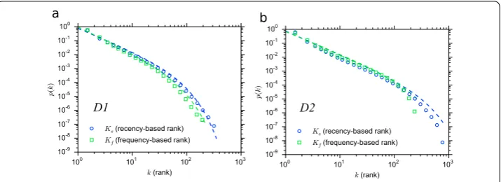
Ks. This analysis shows that such probability decays vary rapidly withKs(Figure ). More
precisely, forD, the probabilityp(Ks) follows a truncated power-law distribution, defined
as
p(x) =Cx–αe–x/κ
with exponentαKs≈.±. and exponential cut-offκKs≈.±. whereas the
best fit for the frequency-based rank distribution is achieved whenαKf ≈.±.
andκKf ≈.±.. ForD, the best fit for the return ranks distribution is obtained with
parametersαKs≈.±. andκKs≈.±. for the recency rank, whereas the
frequency rank has the exponentαKf ≈.±. and cut-offκKf ≈.±. (see
the Supporting Information (Additional file ) for details on the curve fitting methods and results).
Notice that the exponents for the rank distributions were very similar for both datasets, regardless of their significant differences in terms of spatial coverage, number of users and time scale, suggesting that the distribution of the rank variables might be capturing a common underlying mechanism.
However, one can notice that the recency rank is a convolution of both frequencyand
recency biases, since highly-visited locations implies short intervals between visits. In or-der to quantify and decompose the recency bias from the recency rank we explore the intuition that even though lowKf implies lowKs, the opposite is not true. The recency
dimension is memoryless in the sense that theKsvalue of a location at timet+ does not
depend on theKsattand therefore, even recently-discovered locations can have a low
Ks. The following analyses exploit this property of the recency rank by testing whether
infrequently-visited locations can help us identify - and measure - the recency bias.
3.1 Recency over frequency: the role of recent events in human mobility
From the joint distribution of the rank variables we investigated the conditional frequen-cies ofP(Ks|Kf). If users have a bias for recently-visited locations we should observe:
. lower values ofKsmust be frequently observed over a wider range ofKf. It would
suggest that we tend to return to recently-visited locations even if it was just discovered (i.e., lowerKf rank);
. higher values ofKf must deviate from lowerKf values, suggesting that the
probability of return to a location decays with time, especially if it was a highly-visited location.
To test these hypotheses, we analyzedP(Ks|Kf) for allKf andKsvalues. For example, a
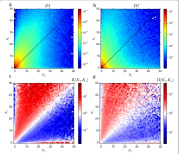
visit to a location with ranks (, ) means a return to the th most visited site after visiting other locations. The conditional frequencies are here represented as two-dimensional histograms (shown as heatmaps) (Figure ).
The first pattern we can observe is that for both datasets the conditional probability distributions (Figure (a) and (b)) are highly skewed and asymmetric. The right-skewness results not only from a combination of the heavy tails ofp(Kf) andp(Ks)
indi-vidually, but also from the convolution of them.
From the asymmetries in the distribution we can extract important insights regarding the dynamics of the recency bias in human mobility. The first one is the fact that recency bias is more pronounced up toKs≈ visits, beyond which the return probability
van-ishes. One possible explanation for such upper bound to the recency effect is due to the maximum long-term temporal regularities observable in D andD (i.e.monthly and yearly respectively). InD, the average number of visits permontha user made is . whereas inD, the average number of visits peryearwas .. Since it is difficult to de-termine the recency bias in such long-term regularities, from here on we will focus our attention on the short-term returns.
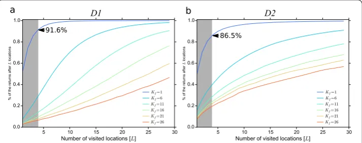
When it comes to our most-visited locations, we tend to return to them after visiting very few locations. It can be seen by the rapid decrease in the returns frequencies when
Ksgrows. For instance, inD, more than % of the returns to the most-visited place
Figure 2 Return probabilities.Each point represents a return, whereas the color encodes the density of points. The top panels correspond to the rank-based recency distribution. The ranks here were shifted to have the highest-ranked locations at (0, 0) and a point (x,y) in the histogram represents a return to the (x+ 1)th most-visited location aftery+ 1 steps.(a)Looking at the return ranks distribution forD1 we can observe that the recency influence is less pronounced inD1 in comparison withD2.(b)On the other hand, the finer-grained data ofD2 shows a strong influence of recency. Return probability ratio(Kf,Ks) forD1(c)and D2(d). In particular, signatures of the dominance of recency should manifest themselves in the plot as red for x>y.
4 The recency bias to recently-discovered locations
As we mentioned before, one way to decompose the recency from the frequency bias is by looking at the returns to recently-discovered or infrequently-visited locations, character-ized by aKf>Cf, whereCf is aKf value above which the recency bias stands out from the
frequency bias in a given dataset. In fact, what we really want to measure is the likelihood of returning to a location whose frequency rank isKf=xafter having visitedKs=y
loca-tions such asp(Kf=x|Ks=y) >p(Kf=y|Ks=x) andxy. Thus, we define the probability
ratio(x,y) as
(x,y) =p(Kf=x|Ks=y)
p(Kf=y|Ks=x)
,
Figure 3 Fraction of returns to theKfmost-visited location occurring after the visitation ofLdifferent
locations.Another way to look at the recency effect is by analyzing the correlation between the number of different visited locations between two visits to a location. We can see that people tend to return to their most-visited locations after visiting very few places.(a)InD1, more than 91% of the returns to the most-visited location occurred after visiting four or fewer locations while forD2(b)it was about 86%.
Cf simply as
Cf=min x
(x,y)|∀y:(x,y) > ;x>y.
From Figures (c) and (d), we can visually estimateCf ≈ andCf≈ forD andD
approximately. Again, as expected, we can observe that the recency bias evident indeed becomes more and more prominent for largerKf.
Based on what we described as the transient nature of the recency effect, it is clear that if a location is recurrently visited within short intervals for a reasonable time, it can climb up positions in theKf rank. Moreover, since the recency information is entirely encoded
within the order in which the places were visited. One simple but very useful implication of this property is that if we randomly shuffle a trajectory, the visitation frequencies are preserved whereas the recency bias is lost.
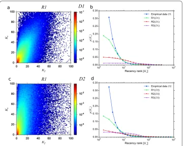
The first feature we can observe is that when we shuffle the trajectories in D (Fig-ure (a)), the ranks distribution exhibit a similar pattern as observed on the original data. However, it supports our claim that the predominance of the preferential return, as cap-tured by the aggregated mobile phone data ofD, is hindering the micro-level dynamics characteristic of the recency effect. A closer look at the bottom rows of Figure (a) does not show any increased probability due to recency. When we artificially destroy the power-law distribution of the visitation frequencies (Figure (b)) we can observe a dramatic change in the ranks distribution. It suggests that a significant part of the ranks distribution ofD is indeed rooted on the visitation frequencies, as predicted by the PR mechanism.
When we analyze the randomized versions ofD the influence of the recency becomes even more evident. As before, shuffling the individuals trajectories (Figure (d)) removes the features we described in Figure (as before, the evidence in the bottom rows is not there). Moreover, by removing the temporal information from visitation sequences inD, the rank distributions acquire the same form as the one ofD.
Figure 4 The rank-based analyses of randomized versions of the empirical datasets. (a)and(c) Conditional probabilities distribution of the randomized versionR1 ofD1 andD2 respectively (additional plots for the other randomization methods are on the Supporting Information). Rank variables were extracted from randomized versions of the datasets. Overall, the conditional probabilities have similar patterns as observed on the original data. However, when we look at theKsdistribution (in log-linear scale) ((b)and(d)), we see that the shuffled data deviates from the empirical data forKs≤4. It is interesting to observe that whenKs> 4 the distributions forR1 and the original data converge again into a single curve.
striking, however, is the fact that this analysis not only shows that the recency effect is bounded to the most recently-visited locations but also suggests a possible existence of an upper limit to the effect. For instance, the recency effect could be observed more strongly when returns occur after visiting two locations inD and three locations inD. It means that if an individual returns to a recently-discovered location before having visited other locations, it is likely that this location will be visited again soon.
5 The recency-based model
Figure 5 Recency-based individual mobility model. Notice that the exploration mechanism is kept the same as in the EPR model. In addition to the PR mechanism, the proposed model incorporates the recency effect, where recently-visited locations have also a high visitation probability.
The model can be described as follows: first, a population ofNagents is initialized and scattered randomly over a discrete lattice withM×Mcells, each one representing a pos-sible location. The initial position of each agent is accounted as its first visit. At each time step agents can visit a new location if probabilitypnew=ρS–γ, where Scorresponds to
the number of distinct locations visited thus far. The parameters values were estimated from the empirical data (see Supporting Information for details) as γD = .±.
and ρD= .±.. ForD, the estimated parameters were γD = .±. and
ρD= .±..
With complementary probability –pnewan agent returns to a previously visited
loca-tion. If the movement is selected to be a return, with probability –αtheith last visited location is selected from a Zipfian distribution (Zipf ’s law) with probability
p(i)∝Ks(li)–η,
where Ks(li) is the recency-based rank of the locationli. The parameter ηcontrols the
number of previously visited locations a user wouldconsiderwhen deciding to visit a lo-cation. With probabilityαthe destination is selected based on the visitation frequencies with probability
i∝Kf(li)––γ,
whereKf(li) is the frequency rank of locationli. Notice that whenα= we recover the
original preferential return behavior of the EPR model while whenα= , visitation re-turns will be based solely on the recency. We experimentally tested different parameters configuration for the model. Our analyses have shown that whenα= , the heavy tail of the visitation frequency disappears while forα= the power law of the recency distribu-tion vanishes.It suggests that both mechanisms must be present in order to reproduce those two features.
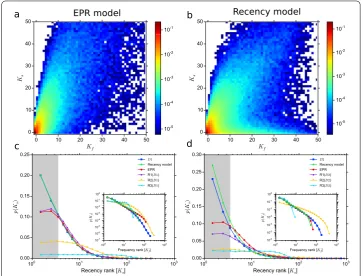
The synthetic data produced by the EPR model seems to have a good approximation with the empirical data (see Figure (a)). However, when we compare the bottom-most rows of the histogram, it deviates from the empirical evidence, by not capturing the broader distribution of p(Kf,Ks) for recently-visited locations. On the other hand, the
recency-based mechanism (RM) reproduced the recency influence as observed in the empirical data (Figure (b)).
When we look at theKf distribution, the EPR model recovers its heavy tail, as one would
Figure 6 Comparison between the EPR model and the recency-based (RM) model. (a)The analysis of the return ranks generated by the EPR model shows that it reproduces a pattern similar to the one observed from the empirical analysis, especially ofD1.(b)On the other hand, on the presence of the recency mechanism, we can observe the same high probability of return to recently-visited locations (i.e., lowKs) as observed on the empirical data.(c)When we look at the distribution of the frequency ranks, the preferencial return mechanisms (labelledEPR) successfully exhibited a power-law distribution, in agreement with the empirical observations. Since theR1 data maintains the visitation frequencies, theKfdistribution of both variables are identical and hence their curves overlap. The activation of the recency mechanism does not affect the frequency rank distribution.(d)However, when we look at theKsdistribution, the EPR mechanism does not capture the power-law behavior observed on the empirical data.
we notice that theKsdistribution, as produced by the EPR model deviates from a power
law. In fact, it is better approximated by an exponential distribution whereas recency-model maintains its power-law behavior. The differences in the Ks distribution as
pro-duced by both models become more evident in log-linear scale, where we can clearly see that the EPR model does not capture the preference for recently-visited locations (see main plot of Figure (c) and Figure (d)).
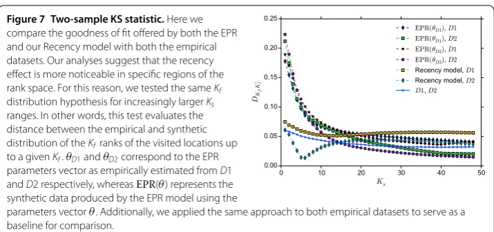
The validity of our approach in reproducing the recency bias was tested using a two-sample Kolmogorov-Smirnov (KS) test. As previously discussed, one way to observe the recency bias is by looking at the distribution ofKf for small Ks. Hence we tested the
same-distribution hypothesis ofKfby comparing the empirical distributions from the data
against those produced by the simulation models. In other words, we want to compare the visitation frequencies of the locations being visited after visits to at leastKslocations
(Figure ). To serve as a reference we applied the same approach comparing theKf
distri-butions ofD againstD.
We can clearly see that the Recency model was the only one to reproduce theKf
distri-bution for smallKsvalues (i.e., the recently-visited locations). Although the fullKf
Figure 7 Two-sample KS statistic.Here we compare the goodness of fit offered by both the EPR and our Recency model with both the empirical datasets. Our analyses suggest that the recency effect is more noticeable in specific regions of the rank space. For this reason, we tested the sameKf distribution hypothesis for increasingly largerKs ranges. In other words, this test evaluates the distance between the empirical and synthetic distribution of theKfranks of the visited locations up to a givenKf.θD1andθD2correspond to the EPR parameters vector as empirically estimated fromD1 andD2 respectively, whereasEPR(θ) represents the synthetic data produced by the EPR model using the
parameters vectorθ. Additionally, we applied the same approach to both empirical datasets to serve as a baseline for comparison.
reproduce recency effect as captured by conditional frequencies. For largerKsvalues (e.g.,
greater than ), theEPRapproximates again to the data, showing a fit even better than our approach, showing that the recency effect is indeed bounded.
Another interesting pattern observed in Figure is that the goodness-of-fit test not only confirmed our findings that the importance of the Recency bias decays as we visit more locations between consecutive visits, but also it supports the evidence that such influence is bounded to approximately five locations.
6 Discussion
When it comes to visitation patterns, humans are extremely regular and predictable, where recurrent travels respond for most of our movements. An external observer can identify from ones’s trajectories locations such as home and work, even after a very short period of observation. On the long term, however, these visitation patterns are not expected to remain the same. New locations are discovered. New social ties are established. New op-portunities arise.
Akin to other human behaviors, traveling patterns evolve from the convolution between internal and external factors. A better understanding on the mechanisms responsible for transforming and incorporating individual events into regular patterns is of fundamental importance. In this work, we revealed that the recency bias - as observed in other human behaviors - also plays a role in human traveling patterns. Our results show that a single visit to a place strongly affects its likelihood of the further visits. More surprisingly, the recency influence is highly bounded to a few recently-visited locations. Our findings were drawn from a novel bivariate rank-based approach from which we could decompose the recency and frequency dimensions in determining individual visitation patterns.
7 Materials and methods
7.1 The empirical datasets
In this work, we used two mobility datasets: the first one (D) corresponds to months of anonymized mobile-phone traces from a large metropolitan area in Brazil. This dataset is composed of ,, records from , users between January -June , . The second dataset (D) is composed of ,,check-insfrom , Brightkite users in , different locations. Unlike the mobile phone data, locations in the Brightkite dataset correspond to the actual places where the users checked in - phone data locations correspond to the antenna tower the phone communicates with and hence are approxi-mations of the user’s actual location.
Since our interest here is on the individuals’trajectories, in this analysis we considered only the data that provides information relating to the users’ displacements. Hence, we fil-tered out multiple repeated observations on the same place, resulting in a time series for each individual, representing their trajectories over the observed period. The rationale for removing the successive points in a same location is because in the context of this work,
recencyis defined in terms of visits to recent past destinations. Hence, successive obser-vations within the same location cannot be considered as being influenced by a recency bias. Thus, since human displacements are interspersed by longer periods with no jumps, the bursty behavior, observed in many human activities (including mobile phone com-munications) [, ] would otherwise wrongfully boost the measurements of a recency preference.
To illustrate how the filtering works, if we assume thatA,BandCare locations, and the data shows a user in the locations (in this order) [A,B,B,B,C,C,A,A,A,B], the multiple consecutive observations at the same locations are filtered out. Hence, the trajectory to be analyzed would be [A,B,C,A,B]. Furthermore, to reduce the influence of co-located an-tennas (common in densely-populated sites), we merged those within less than meters apart under the just one id.
7.2 The randomized datasets
Additionally, in order to verify whether the power law observed in the recency rank dis-tribution is rooted on the temporal semantics of individuals’ trajectories, we applied our rank-based approach to randomized versions of both empirical datasets (D andD). The first randomized dataset we analyzed (R) was obtained from uniformly shuffling each individual trajectory. This way, we artificially remove any temporal information possibly encoded within the individual trajectories, while maintaining the visitation frequencies in-tact. On the second randomization method (R), we also remove the visitation frequencies by generating for each user a new random trajectory with the same number of displace-ments, and the same number of distinct visited locations. To serve as the baseline for the analyses, the data of the third randomization approach (R) produces a new dataset with the same size as the original one, but keeping only the total number of users and locations. More precisely, for each of the datasets, we generated a randomized version of them with
Mrandom points
vm= [um,lm,m], m∈[, . . . ,M],
where eachum,lmis uniformly sampled fromUusers andNlocations respectively, with
Additional material
Additional file 1: Supporting Information: Statistical analysis and parameters estimation(pdf )
Competing interests
The authors declare that they have no competing interests.
Authors’ contributions
Developed the ideas, methods and analyses: HB and RM. Empirical data analysis: HB and AE. Wrote the manuscript: HB, FBLN and RM.
Author details
1BioComplex Lab, Florida Institute of Technology, 150 W University Blvd, Melbourne, FL 32901, USA.2Computational Intelligence Research Group, Polytechnic School, University of Pernambuco, Rua Benfica, 455, Recife, PE, 50720-001, Brazil. 3COPPE, Federal University of Rio de Janeiro, Rua Horácio Macedo, Bloco G, 2030-101, Rio de Janeiro, RJ, 21941-450, Brazil.
Endnote
a Brightkite was a location-based social networking service launched in 2007 and closed in 2011 [33, 42].
Received: 24 July 2015 Accepted: 11 November 2015
References
1. Belik V, Geisel T, Brockmann D (2011) Natural human mobility patterns and spatial spread of infectious diseases. Phys Rev X 1(1):011001. doi:10.1103/PhysRevX.1.011001
2. Colizza V, Barrat A, Barthelemy M, Valleron A-J, Vespignani A (2007) Modeling the worldwide spread of pandemic influenza: baseline case and containment interventions. PLoS Med 4(1):13. doi:10.1371/journal.pmed.0040013 3. Balcan D, Vespignani A (2011) Phase transitions in contagion processes mediated by recurrent mobility patterns. Nat
Phys 7:581-586. doi:10.1038/nphys1944
4. Toole JL, Ulm M, González MC, Bauer D (2012) Inferring land use from mobile phone activity. In: Proceedings of the ACM SIGKDD international workshop on urban computing. ACM, New York, pp 1-8. arXiv:1207.1115v1
5. Lenormand M, Gonçalves B, Tugores A, Ramasco JJ (2015) Human diffusion and city influence. J R Soc Interface 12:20150473. arXiv:1501.07788
6. Kitamura R, Chen C, Pendyala R, Narayanan R (2000) Micro-simulation of daily activity-travel patterns for travel demand forecasting. Transportation 27(1):25-51
7. Jung W, Wang F, Stanley H (2008) Gravity model in the Korean highway. Europhys Lett 81(4):48005. arXiv:0710.1274v1 8. Krajzewicz D, Hertkorn G, Wagner P, Rössel C (2011) SUMO (Simulation of Urban MObility): an open-source traffic
simulation car-driver model
9. Song C, Qu Z, Blumm N, Barabási A-L (2010) Limits of predictability in human mobility. Science 327(5968):1018-1021. doi:10.1126/science.1177170
10. Wang D, Pedreschi D, Song C, Giannotti F, Barabási A-L (2011) Human mobility, social ties, and link prediction. In: Proceedings of the 17th ACM SIGKDD international conference on knowledge discovery and data mining - KDD ’11. ACM, New York, p 1100. doi:10.1145/2020408.2020581
11. Yang Y, Herrera C, Eagle N, González MC (2014) Limits of predictability in commuting flows in the absence of data for calibration. Sci Rep 4:5662. doi:10.1038/srep05662
12. Sadilek A, Krumm J (2012) Far out: predicting long-term human mobility. In: Twenty-sixth AAAI conference on artificial intelligence, pp 814-820
13. Krumme C, Llorente A, Cebrian M, Pentland AS, Moro E (2013) The predictability of consumer visitation patterns. Sci Rep 3:1645. doi:10.1038/srep01645
14. Lu X, Wetter E, Bharti N, Tatem AAJ, Bengtsson L (2013) Approaching the limit of predictability in human mobility. Sci Rep 3:2923. doi:10.1038/srep02923
15. González MC, Hidalgo CA, Barabási A-L (2008) Understanding individual human mobility patterns. Nature 453(7196):479-482. doi:10.1038/nature06958
16. Brockmann D, Hufnagel L, Geisel T (2006) The scaling laws of human travel. Nature 439(7075):462-465. doi:10.1038/nature04292
17. Hasan S, Schneider CM, Ukkusuri SV, González MC (2012) Spatiotemporal patterns of urban human mobility. J Stat Phys 151:304-318. doi:10.1007/s10955-012-0645-0
18. Song C, Koren T, Wang P, Barabási A-L (2010) Modelling the scaling properties of human mobility. Nat Phys 6(10):818-823. doi:10.1038/nphys1760
19. Schneider CM, Belik V, Couronné T, Smoreda Z, González MC, Couronne T (2013) Unravelling daily human mobility motifs. J R Soc Interface 10:20130246. doi:10.1098/rsif.2013.0246
20. Merton RK (1968) The Matthew effect in science: the reward and communication systems of science are considered. Science 159(3810):56-63. doi:10.1126/science.159.3810.56
21. Price D (1976) A general theory of bibliometric and other cumulative advantage processes. J Am Soc Inf Sci 27(5):292-306
22. Barabási A-L, Albert R (1999) Emergence of scaling in random networks. Science 286(5439):509-512. doi:10.1126/science.286.5439.509
24. Toole JL, Herrera-Yaque C, Schneider CM, González MC (2015) Coupling human mobility and social ties. J R Soc Interface 12(105):20141128. doi:10.1098/rsif.2014.1128
25. Weber EU, Johnson EJ (2006) Constructing preferences from memory. doi:10.2139/ssrn.1301075
26. Hoch SJ (1984) Availability and interference in predictive judgment. J Exp Psychol Learn Mem Cogn 10(4):649-662. doi:10.1037/0278-7393.10.4.649
27. Hoch SJ (1985) Counterfactual reasoning and accuracy in predicting personal events. J Exp Psychol Learn Mem Cogn 11(4):719-731. doi:10.1037/0278-7393.11.1-4.719
28. Huang W, Li S, Liu X, Ban Y (2015) Predicting human mobility with activity changes. Int J Geogr Inf Sci 29(9):1569-1587. doi:10.1080/13658816.2015.1033421
29. Zheng Y, Zhang L, Xie X, Ma W (2009) Mining correlation between locations using human location history. In: Proceedings of the 17th ACM SIGSPATIAL international conference on advances in geographic information systems, pp 2-5. doi:10.1145/1653771.1653847
30. Zheng Y, Zhang L, Xie X, Ma W-Y (2009) Mining interesting locations and travel sequences from GPS trajectories. In: Proceedings of the 18th international conference on world wide web - WWW ’09, pp 791-800.
doi:10.1145/1526709.1526816
31. Lichman M, Smyth P (2014) Modeling human location data with mixtures of kernel densities. In: Proceedings of the 20th ACM SIGKDD international conference on knowledge discovery and data mining - KDD ’14, pp 35-44. doi:10.1145/2623330.2623681
32. Yan X, Zhao C, Fan Y, Di Z, Wang W (2013) Universal predictability of mobility patterns in cities. J R Soc Interface 11:20140834. doi:10.1098/rsif.2014.0834
33. Cho E, Myers SA, Leskovec J (2011) Friendship and mobility. In: Proceedings of the 17th ACM SIGKDD international conference on knowledge discovery and data mining - KDD ’11. ACM, New York, p 1082.
doi:10.1145/2020408.2020579
34. Zhang D, Xiong H, Yang L, Gauither V (2013) NextCell: predicting location using social interplay from cell phone traces. IEEE Trans Comput. doi:10.1109/TC.2013.223
35. Smoreda Z, Olteanu-Raimond AM, Couronné T (2013) Spatiotemporal data from mobile phones for personal mobility assessment. In: Zmud J et al (eds) Transport survey methods: best practice for decision making. Emerald, Bingley, pp 745-768
36. Wang P, Hunter T, Bayen AM, Schechtner K, González MC (2012) Understanding road usage patterns in urban areas. Sci Rep 2:1001. doi:10.1038/srep01001
37. Gambs S, Killijian M-O, Del Prado Cortez MNN (2012) Next place prediction using mobility Markov chains. In: Proceedings of the first workshop on measurement privacy and mobility MPM 2012, pp 1-6.
doi:10.1145/2181196.2181199
38. Herder E, Siehndel P, Kawase R (2014) Predicting user locations and trajectories. In: User modeling, adaptation, and personalization. Springer, Cham, pp 86-97
39. Song L, Kotz D, Jain R, He X (2006) Evaluating next-cell predictors with extensive Wi-Fi mobility data. IEEE Trans Mob Comput 5(12):1633-1648. doi:10.1109/TMC.2006.185
40. Karsai M, Kaski K, Barabási A-L, Kertész J (2012) Universal features of correlated bursty behaviour. Sci Rep 2:397. doi:10.1038/srep00397
41. Jo HH, Karsai M, Kertesz J, Kaski K (2012) Circadian pattern and burstiness in mobile phone communication. New J Phys 14:013055. doi:10.1088/1367-2630/14/1/013055