Evaluating the performance of sentence level features and domain sensitive features of product reviews on supervised sentiment analysis tasks

(1)

Evaluating the performance of sentence

level features and domain sensitive features

of product reviews on supervised sentiment

analysis tasks

Bagus Setya Rintyarna

1,2*

_{, Riyanarto Sarno}

1

_{and Chastine Fatichah}

1

Introduction

The exponential growth of e-commerce has triggered it to become a rich source of infor-mation nowadays. On e-commerce, customers provide a qualitative evaluation in the

form of an online review that describes their opinions on a specific product [1]. With

a huge number of OPRs, manual processing is not an efficient task. Sentiment analysis (SA) technique emerges in response to the requirement of processing OPRs in speed

[2]. In terms of product review analysis, SA which is also named Opinion Mining can

be defined as a task of recognizing customer’s opinion or sentiment toward the prod-ucts or the product features [3] that can be categorized into positive, negative, or neutral

Abstract

With the popularity of e-commerce, posting online product reviews expressing customer’s sentiment or opinion towards products has grown exponentially. Senti-ment analysis is a computational method that plays an essential role in automating the extraction of subjective information i.e. customer’s sentiment or opinion from online product reviews. Two approaches commonly used in Sentiment analysis tasks are supervised approaches and lexicon-based approaches. In supervised approaches, Sentiment analysis is seen as a text classification task. The result depends not only on the robustness of the machine learning algorithm but also on the utilized features. Bag-of-word is a common utilized features. As a statistical feature, bag-of-word does not take into account semantic of words. Previous research has indicated the potential of semantic in supervised SA task. To augment the result of sentiment analysis, this paper proposes a method to extract text features named sentence level features (SLF) and domain sensitive features (DSF) which take into account semantic of words in both sentence level and domain level of product reviews. A word sense disambiguation based method was adapted to extract SLF. For every similarity employed in generating SLF, the SentiCircle-based method was enhanced to generate DSF. Results of the exper-iments indicated that our proposed semantic features i.e. SLF and SLF + DSF favorably increase the performance of supervised sentiment analysis on product reviews. Keywords: Sentiment analysis, Online product reviews, Supervised approach, Machine learning

Open Access

© The Author(s) 2019. This article is distributed under the terms of the Creative Commons Attribution 4.0 International License (http://creat iveco mmons .org/licen ses/by/4.0/), which permits unrestricted use, distribution, and reproduction in any medium, provided you give appropriate credit to the original author(s) and the source, provide a link to the Creative Commons license, and indicate if changes were made.

RESEARCH

*Correspondence: bagus.setya@unmuhjember. ac.id

2_{Department of Electrical}

Engineering, Universitas Muhammadiyah Jember, Jember, Indonesia

(2)

responses [4]. SA plays an important role to automate the extraction of subjective infor-mation i.e. sentiment embodied in OPRs. The success of SA application on product

reviews will in turn help customers in suggesting about buying a certain product [5]

based on the analysis of OPRs. Meanwhile, for companies and online marketers, they can make use SA technique to foresee customer satisfaction toward a certain product

[6]. Two major approaches commonly employed for SA tasks on product reviews are

lexicon-based approaches and ML-based approaches [7]. In extracting opinions or

senti-ments from the text data, lexicon-based methods rely on a sentiment lexicon e.g.

Sen-tiwordNet [8], SO-CAL [9], MPQA subjectivity lexicon [10], Harvard general inquirer,

Bing Liu’s opinion lexicon [11], SenticNet [12], and NRC emotion lexicon [13].

Senti-ment lexicon is a dictionary of precompiled sentiSenti-ment terms [14]. Sentiment term is

term, commonly verb and adjective, representing the sentiment of the text document. In brief, lexicon-based method extract all sentiment terms for any given text and assign their sentiment value using sentiment lexicon. Meanwhile, ML-based techniques rely on ML algorithms and see SA as a regular text classification task. Text classification task

assigns a piece of text data into several predefined classes involving ML algorithms [15].

In terms of SA task, ML-based techniques classify text document into one out of three classes namely positive class, neutral class, and negative class. For a given set of training text data, ML algorithms build a model based on the extracted features of a labeled text. The model is then utilized to classify unlabeled text. The result of supervised SA task is therefore influenced by the robustness of both extracted text features and ML

algo-rithms. Mostly, recent works [16–19] dealing with supervised SA concerned more on

the extension of the employed ML algorithms instead of the development of robust text

features. We briefly overview those works on “Related work” section. Concerning on the

extraction of text features is therefore still challenging task in the area of supervised SA. Referring to the previously research gap, the motivation for this study comprises:

1. Enhancing the result of supervised SA by proposing a method to extract robust text features for supervised SA task.

2. Evaluating the performance of the proposed text features using several ML-algo-rithms and feature selection methods.

In proposing the method to extract text features for supervised SA, we consider the

finding reported by [3]. Rintyarna [3] highlighted the importance of semantics for SA

task. Taking into account semantics of words is important for SA since the same term appears in different text data may reveals different meaning i.e. different sentiment value. In turn, capturing sementics is potential to augment the result of Sentiment Anal-ysis task. In this study, we present a method to extract text features capturing semantic in sentence level and domain level of product reviews. We introduce two feature sets namely sentence level feature (SLF) and domain sensitive feature (DSF). For extracting

SLF, a WSD based technique was adapted [20]. And for extracting DSF, a Senti-Circle

(3)

and feature selection methods. The result of experiment indicated that our proposed features outperformed BOW.

The rest of the manuscript is arranged in the following sections. “Related work”

sec-tion reviews state of the art study related with this work. “Proposed method” section

describes the proposed method for extracting SLF and DLF. We explore the result of

experiment and the discussion in “Experimental results and discussion” section. Finally

we summarize the result of this work in “Conclusion” section.

Related work

Using BOW, [16] performed an SA task on an Amazon product review dataset. RFSVM,

a hybrid method that combines Random Forest (RF) and Support Vector Machine (SVM), was employed to make use of the capabilities of both classifiers. Precision, recall, F-Measure, and accuracy were used as the performance metrics to evaluate the pro-posed method compared with the baseline methods i.e. RF and SVM. Using instances of 500 positive datasets and 500 negative datasets, the result of the experiment showed that RFSVM outperformed the baseline methods in terms of all three performance metrics.

A word embedding-based sentiment classification is proposed [17]. Using google

toolkit word2vec, a continuous bag-of-words (CBOW) model and a Skip-gram model were generated in order to produce meaningful features. For representing the document, the sum of weighted word embeddings was used. Combined with SVM, this work pro-posed an extension of the SVM classifier, called SVM-WE. The method was evaluated using four datasets i.e. RT-s, CR, RT-2k, and IDBM. The result of the experiment indi-cated that the proposed method performed slightly better compared with the baseline method.

Another work [18] proposed a set of 13 sentiment features for supervised SA in

Twit-ter dataset classification. Features F1 to F8 were generated based on three sentiment lexicons, i.e. SenticNet, SentiWordNet, and NRC Emotion Lexicon. Features F9 to F13 were generated using a seed word list i.e. Subjective Words. Two datasets, namely TaskA Twitter and TaskB Twitter, were employed to validate feature performance in classifica-tion. The Naïve Bayes classifier was used as performance metric to calculate its accuracy. The best accuracy achieved by the proposed features was 75.60%.

In order to analyze social media content, Yoo [19] proposed a system to predict user

sentiment. For representing the text data, the work adopted a two-dimensional rep-resentation of word2vec. The model for the sentiment analysis task was built using Convolutional Neural Network for Sentence Classification (CNN) by making use of TensorFlow, an open-source library for various dataflow programming tasks. Validated using the Sentiment140 dataset, containing 800,000 positive documents and 800,000 negative documents, the proposed model outperformed th baseline method i.e. Naïve Bayes, SVM, and Random Forest.

As an utmost advanced topic in the field of Natural Language Processing

(NLP), many approaches have been developed for SA application [21]. Among

(4)

determining the product features that require improvement [22]. In the following paragraphs we briefly review several works discussing ABSA.

A method called joint aspect-based sentiment topic (JABST) has been introduced

[23]. It proposed a unified framework to perform common ABSA task including

aspect extraction and sentiment polarity identification. The study made use graphi-cal model to describe relationship among aspects, opinion, sentiment polarity and granularity. A maximum entropy based model called MaxEnt-JABST has also been proposed to improve the word distribution description. In the evaluation step, two

real world datasets from [24] were employed. The evaluation step focused on two

points i.e.: (1) comparing the quality of the extracted topics and (2) calculating the precision of aspects and opinions. The results of experiment confirmed that the JABST significantly outperformed baseline model.

To perform ABSA tasks on customer reviews, a novel system called W2VLDA

was presented by [25] based on the combination of a topic modeling approach and a

Maximum Entropy classifier. The system performed the main tasks of ABSA simul-taneously. Employing Brown cluster to train the model of Maximum Entropy clas-sifier, W2VLDA was able to separate aspect-terms and opinion-words into word classes without any language dictionary. The work conducted experiment to evalu-ate the performance of different subtasks using different datasets. Restaurant review

dataset [26] containing domain-related aspects was used to evaluate aspect category

classification. Dataset on the domain of Laptops and Digital-SLR [24] containing

English reviews was employed to evaluate sentiment classification subtask.

Mean-while, SemEval-2016 task 5 from [27] was used to perform multilingual experiments.

Compared with the other LDA-based approaches as baseline methods, the system achieved slightly better results.

Another work [28] focused on three subtasks of ABSA i.e.: sentiment extraction,

aspect assignment, and aspect category determination. The work contributed to improving the functionality of the current state-of-the-art topic model approach by adding product description as another dimension of the model. Two extended topic model-based ABSA methods were presented: Seller-aided Aspect-based Sentiment Model (ASM) and Seller-aided Product-based Sentiment Model (PSM). SA-ASM outperformed two baseline methods on sentiment classification and aspect assignment. Meanwhile, SA-PSM performed better compared with the baseline methods on subtask aspect categorization.

Aspect extraction which aims at identifying the object of user’s opinion from online reviews holds an important role in ABSA approach. Motivated by the vul-nerability of syntactic patterns-based approach due to its dependency to

depend-ency parser, a study [29] proposed two-fold rule-based model (TF-RBM) to perform

ABSA tasks. Sequential pattern-based rules (SPR) [30] was firstly employed to

(5)

Proposed method

The steps of the proposed method are: (1) capturing semantic values in product review texts at the sentence level and extracting the sentence level features (SLF), (2) capturing semantic values in product reviews influenced by different product domain extracting the domain sensitive features (DSF). Since there are many notations employed in this section, we present details of the notations in Table 1.

Extracting sentence level feature (SLF)

Capturing sentence-level semantic is important since the same words that appear in different piece of text may share different meaning i.e. different sentiment value as

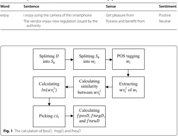
described in Table 1. In Table 2, we describe that the word “enjoy” has different sense

i.e. different sentiment value when it appears in different sentence. This characteristic is known as polysemy. The task aims at assigning correct sentiment value to a word with respect to its local context i.e. sentence. We describe the step of extracting SLF in Fig. 1.

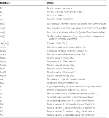
Table 1 Details of notations

Notations Details

D Product review document

Sk Review sentence within D with index-k

wi Word with index-i

wsj_i Sense of word i with index-j

sposj_i Raw positive sentiment value of wsj_i picked from SentiwordNet

snegj_i Raw negative sentiment value of wsj_i picked from SentiwordNet

sneuj_i Raw neutral sentiment value of wsj_i picked from SentiwordNet

simcd

ab Similarity value between wsca and wsdb calculated using one of

Wordnet similarity algorithms

deg

wsj_i

Indegree score of wsj_i

csposi Contextual positive sentiment value of wi

csnegi Contextual negative sentiment value of wi

csneui Contextual neutral sentiment value of wi

fposSk Positive value of feature of Sk

fnegSk Negative value of feature of Sk

fneuSk Neutral value of feature of Sk

fposD Positive value of feature of D

fnegD Negative value of feature of D

fneuD Neutral value of feature of D

wd Domain word of product review dataset

pwk Pivot word of review sentence Sk

θ_i Angle representing semantic orientation adjustment of wi

ri Degree of correlation between pwk and wi

ctsi Prior sentiment value of wi determined using Rule (11)

xi Senticircle representation in Cartesian coordinate

yi Senticircle representation in Cartesian coordinate

fxSk Feature value of Sk calculated using x of Senticircle

fySk Feature value of Sk calculated using y of Seinticircle

fxD Feature value of D calculated using x of Senticircle

(6)

To capture semantic value in product reviews at sentence level i.e. extracting SLF,

product review document D is split into review sentence Sk . The process is done at

sentence level. Suppose Sk consists of n words, w1,w2,. . .wn . The aim of this stage

is to find contextual sentiment value csi of word wi associated with sentiment score

si picked from SentiwordNet [8]. In the next step, part of speech (POS) tagging is done, which is part of common text processing, including filtering. It is a process of

assigning a part of speech value to a word in a piece of text [31]. Since we employ

Sen-tiwordNet [8], which is based on WordNet [32], POS tagging is important for

select-ing the correct sense of wi in accordance with its POS tag [33]. WordNet [32] itself

employs 4 POS tags, i.e. noun, verb, adjective, and adverb. POS tagging is important

for the next step, i.e. extracting wsj_i from wi . For every extracted wsj_i its associated

sen-timent value is picked from SentiwordNet [8]. Every wsji has three different sentiment

scores, namely sposj_i, sneg_ij, and sneuj_i.

The similarity between wsj_i is calculated using WordNet similarity algorithms, i.e. from Lin, Jiang and Conrath, Resnik, Leacock and Chodorow, and Wu and Palmer. Adapted Lesk [34] is also employed. Similarity between word senses, denoted as simcd_ab , means

similarity value of wsca and wsd_b . They are calculated for all possible combinations, as

can be seen in Table 3. The calculation adopts the WSD technique firstly introduced by

[20]. For simple, the task illustrated in Table 4 can be assumed as building undirected

weighted graph of every review sentence with ws_ij as the vertex and simcd_ab as the weight of the edges of the graph.

The results of the previous step are the three different sentiment scores from

Senti-WordNet [8]. For example, the result of processing the review sentence ‘The screen is

Table 2 Example of different sentiment of the word “enjoy”

Word Sentence Sense Sentiment

enjoy I enjoy using the camera of this smartphone Get pleasure from Positive The vendor enjoys new regulation issued by the

authority Possess and benefit from Neutral

Splitting

into Splitting into POS tagging

Extracting of Calculating

similarity between Calculating

Picking Calculating

and

(7)

great’, can be seen in Table 4. After the POS tagging step, including filtering, there are two words, i.e. ‘screen’ with POS tag noun and ‘great’ with POS tag adjective.

To assign csi of wi , the indegree score of wsij , denoted by In

wsj_i , is calculated. Inde-gree score is important to assign contextual sense of wi . Among the senses of wi i.e. wsj_i , a sense with the highest Indegree score is assigned as contextual sense of wi . Contextual sense is a sense where csposi, csnegi, and csneui are picked from the collection of

Senti-wordNet and assigned as contextual sentiment value of wi . For the above case there are

three indegree scores for w1 , i.e. deg ws₁1

, deg ws2₁

and deg

ws3₁

while there are two indegree scores for w2 , i.e. deg

ws1₂

and deg ws2₂

. They are calculated as follows:

deg(ws1₁)=sim11₁₂+sim12₁₂

deg

ws2₁

=sim21₁₂+sim22₁₂

degws3₁=sim31₁₂+sim32₁₂.

Table 3 Similarity between word senses

w1 w2

ws1 1 ws 2 1 ws 3 1 ws 1 2 ws 2 2

w1 ws1

1 sim1112 sim1212

ws2

1 sim2112 sim2212

ws31 sim3112 sim3212

w2 ws1 2 ws2 2

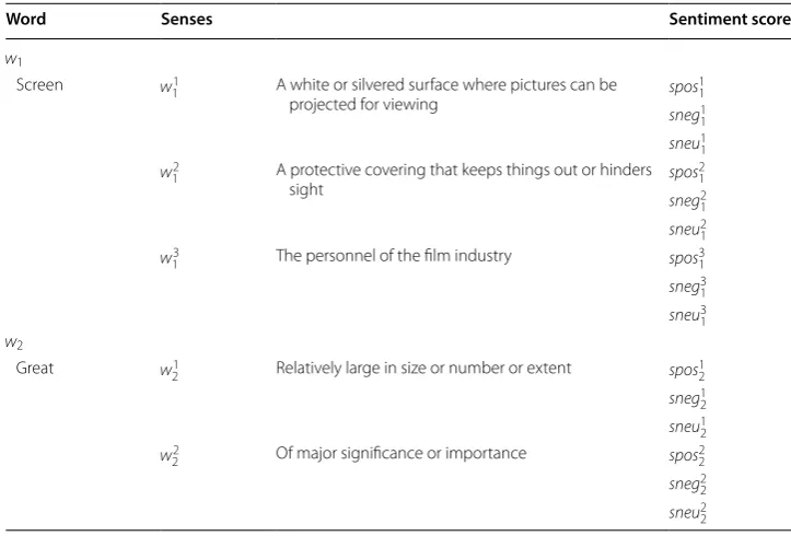
Table 4 Word senses along with their sentiment score

Word Senses Sentiment score

w1

Screen w1

1 A white or silvered surface where pictures can be

projected for viewing spos

1 1 sneg1 1 sneu1 1 w2

1 A protective covering that keeps things out or hinders

sight spos

2 1 sneg21

sneu2 1

w3

1 The personnel of the film industry spos31

sneg3 1 sneu3 1

w2

Great w₂1 Relatively large in size or number or extent spos1₂

sneg1 2 sneu12

w2

2 Of major significance or importance spos22

sneg2

2

(8)

The next task is determining the selected sense of wi by calculating

max

deg

ws1 1

, deg

ws2₁

, deg

ws3₁

. The sense that has the highest indegree score is selected as the contextual sense of wi and its sentiment score is labeled with csposi ,

csnegi , or csneui . Once these values have been assigned for every wi, the last procedure

in this step is calculating the numeric feature value at the sentence level, fposSk, fnegSk, and fneuSk , using Eqs. (1), (2) and (3).

where n is the number of words in Sk . To calculate the numeric feature value at review

document level, Eqs. (4), (5), and (6) are employed. For o is the number of sentences in review document D, fposD, fnegD, and fneuD are calculated as follows:

Capturing domain sensitive features (DSF)

In this step, we adopt Senticircle approach [35]. The main principle of Senticircle suggest that terms exist in the same context tend to share the same semantics. In terms of prod-uct review, we define the context as prodprod-uct domain. In consequence, the same terms that appears in different product domains tend to share different meaning. In terms of SA, sharing different meanings means carrying different sentiment. For example, ‘long battery life’ in Electronics domain express positive sentiment, while ‘long stopping time’ in the Automobile domain share negative sentiment.

To generate the DSF, several formulas are provided. Figure 2 describes the steps that

need to be carried out. The first three steps, including POS tagging, are the same as in the first step of the method. The next step is determining pivot word pwk of sentence Sk .

(1)

fposSk= n

i=1

csposi

(2) fnegSk =

n

i=1

csposi

(3) fneuSk =

n

i=1

csposi

(4)

fposD=

o

k=1fposSk

k

(5) fnegD=

o

k=1fnegSk

k

(6) fneuD=

o

k=1fneuSk k

(7) maxSim=argmaxSimiSimi(wd,wi)

(8) Simi=

2∗Depth(LCS(wd,wi)) Depth(wd)+Depth(wi)

(9)

A pivot word is a representative of the domain word at sentence level [3]. In this work,

pwk is defined as the noun with the closest similarity to the domain word. For measuring

similarity, Wu and Palmer’s algorithm is employed [36]. For wd as the domain word (e.g.

Smartphone, Book, Beauty, or Computers), the similarity between wd and wi is

com-puted using (7) and (8). The pivot word from wi that has the highest value, maxSim , is selected.

In Eq. (8), LCS means the Least Common Subsumer between the first sense of wd and

the contextual sense of wi in the WordNet [32] taxonomy. Since the method from [37]

was adopted in this stage, ri is computed to represent the distance between wi and pwk

using Eq. (9). In (9), N is the total number of words in the corpus of product reviews and Nwi is the total number of wi.

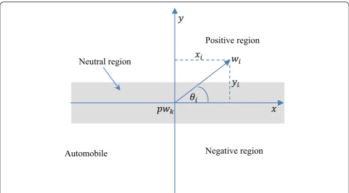
To generate the SentiCircle representation of wi , we need to assign θi using Eq. (10).

In Eq. (10), ctsi is determined using rule (11).

The last step is to generate the SentiCircle representation by using (12) and (13). The sentiment value of a word is represented using the values of x and y in a Cartesian coor-dinate system as seen in Fig. 3. To calculate the numeric value of the features in sentence Sk , Eqs. (14) and (15) are introduced, where NwSk is the number of words in Sk.

(9) ri=f(pwk,wi)log

N Nwi

(10)

θi=ctsi∗πrad

(11)

ctsi=

csposi if |csposi|>

csnegi

csnegi if

csneg_i

>|cspos_i|

(12) xi=ricosθi

(13)

yi=risinθi

(14)

fxSk =

NwSk

i=1 xi

NwSk

Splitting

into Splitting into POS tagging

Determining Calculating

and Calculating

and

Calculating and

(10)

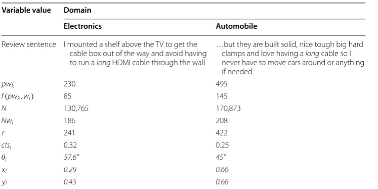
In Fig. 4, we provide an example of how Senticircle adjust a sentiment value of the same word “long” but from different domain e.g. Electronics and Automobile. The

word “long” is picked from review document of the dataset as presented in Table 5. In

Table 5, we also provide the variable value of the Senticircle of the word “long”. In the

first domain e.g. Electronics, the word “long” has relatively neutral value while in the

second domain e.g. Automobile, this word has highly positive value. The value of xi and

yi presented in the table is the value after normalization.

To represent a document with its semantic features, the numeric value of the features in the review document is calculated using Eqs. (16) and (17). In both equations, o is the

number of sentences in D . For every similarity algorithm, a set of features is generated,

(15)

fyS_k =

NwSk

i=1 yi

NwSk

Automobile

Positive region

Negative region Neutral region

Fig. 3 Representation of Senticircle in Cartesian coordinate system

Electronics Automobile

(11)

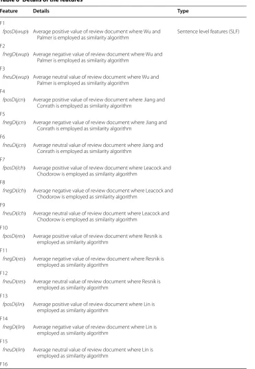
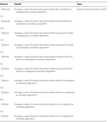
i.e.: fposD , fnegD , fneuD , fxD , and fyD . Since 5 similarity algorithms are employed (Wu and Palmer, Jiang and Conrath, Leacock and Chodorow, Resnik, and Li), the complete set of review document features consists of 25 features, as listed in Table 6. In the table, we describe the notation of the features, the details and the type of the features. F1–F15 is local features. Meanwhile, F16–F25 is domain sensitive features.

Experimental results and discussion

Experimental setup

An experiment was conducted to evaluate the features extracted by the proposed

method employing several machine learning algorithms available in WEKA [38], i.e.

Bayesian Network, Naïve Bayes, Naïve Bayes Multinomial, Logistic, Multilayer Percep-tron, J48, Random forest, and Random tree. Another experiment was conducted using feature selection method. In the implementation, WEKA feature selection methods were employed, i.e.: ClassifierAttributeEval (CA), GainRatioAttributeEval (GR), Info-GainAttributeEval, OneRAttributeEval (OneR) and PrincipalComponent (PCA). Preci-sion, recall and F-measure were calculated as performance metrics. Although important, extending Machine learning algorithms is not part of our contribution. A key point of this work is to demonstrate as well as to evaluate the performance of our proposed semantic features. For that reason, in all experiment we employ default setting of the ML parameters provided by WEKA to avoid bias in the result of experiment. The experi-ments were performed on IBM System X3400 M3 Tower Server.

(16) fxD=

o

k=1Sk

o

(17) fyD=

o

k=1Sk

o

Table 5 Variable value of the word “long” calculated for both domains

Italic values indicate Senticircle parameters calculated in both domains Variable value Domain

Electronics Automobile

Review sentence I mounted a shelf above the TV to get the cable box out of the way and avoid having to run a long HDMI cable through the wall

…but they are built solid, nice tough big hard clamps and love having a long cable so I never have to move cars around or anything if needed

pwk 230 495

f(pwk,wi) 85 145

N 130,765 170,873

Nwi 186 208

r 241 422

ctsi 0.32 0.25

θ_i 57.6° 45°

xi 0.29 0.66

(12)

Table 6 Details of the features

Feature Details Type

F1

fposD(wup) Average positive value of review document where Wu and

Palmer is employed as similarity algorithm Sentence level features (SLF) F2

fnegD(wup) Average negative value of review document where Wu and Palmer is employed as similarity algorithm

F3

fneuD(wup) Average neutral value of review document where Wu and Palmer is employed as similarity algorithm

F4

fposD(jcn) Average positive value of review document where Jiang and

Conrath is employed as similarity algorithm F5

fnegD(jcn) Average negative value of review document where Jiang and Conrath is employed as similarity algorithm

F6

fneuD(jcn) Average neutral value of review document where Jiang and Conrath is employed as similarity algorithm

F7

fposD(lch) Average positive value of review document where Leacock and Chodorow is employed as similarity algorithm

F8

fnegD(lch) Average negative value of review document where Leacock and

Chodorow is employed as similarity algorithm F9

fneuD(lch) Average neutral value of review document where Leacock and Chodorow is employed as similarity algorithm

F10

fposD(res) Average positive value of review document where Resnik is employed as similarity algorithm

F11

fnegD(res) Average negative value of review document where Resnik is employed as similarity algorithm

F12

fneuD(res) Average neutral value of review document where Resnik is

employed as similarity algorithm F13

fposD(lin) Average positive value of review document where Lin is

fnegD(lin) Average negative value of review document where Lin is employed as similarity algorithm

F15

fneuD(lin) Average neutral value of review document where Lin is employed as similarity algorithm

(13)

Dataset description

The experiment was conducted using Amazon product data [39] downloaded from

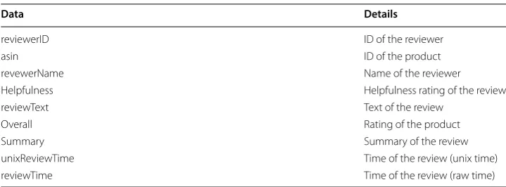
http://jmcau ley.ucsd.edu/data/amazo n/. The collection contains product review data-set grabbed from Amazon including 142.8 millions reviews. The experiment was con-ducted on a small subset of this collection, i.e. the electronics and automobile datasets. The number of sample for building model and running evaluation follow the rule of tenfold cross-validation. The dataset contains reviewerID, asin, reviewerName, helpful-ness, reviewText, overall, summary, unixReviewTime, and reviewTime as described in

Table 7. We pick the review text for experiment from reviewText. To build the ground

truth, we established a label out of three sentiment categories i.e. positive, negative, and neutral for every reviewText based on its overall score. Datasets with overall score 1–2 were assigned as negative reviews. Meanwhile, reviewTexts with overall score 4–5 were labeled positive. And the rest was assigned as neutral review.

Table 6 (continued)

Feature Details Type

fxD(wup) Average x value of review document where Wu and Palmer is

employed as similarity algorithm Domain sensitive features (DSF) F17

fyD(wup) Average y value of review document where Wu and Palmer is

fxD(jcn) Average x value of review document where Jiang and Conrath is employed as similarity algorithm

F19

fyD(jcn) Average y value of review document where Jiang and Conrath is employed as similarity algorithm

F20

fxD(lch) Average x value of review document where Leacock and

Cho-dorow is employed as similarity algorithm F21

fyD(lch) Average y value of review document where Leacock and Cho-dorow is employed as similarity algorithm

F22

fxD(res) Average x value of review document where Resnik is employed as similarity algorithm

F23

fyD(res) Average y value of review document where Resnik is employed as similarity algorithm

F24

fxD(lin) Average x value of review document where Lin is employed as similarity algorithm

F25

(14)

Results and discussion

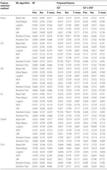
Three scenarios were arranged for the experiment, i.e. (1) using a baseline features i.e. BoW (BF) that is commonle employed for recent supervised sentiment analysis task, (2) using sentence level feature only (SLF), and (3) using sentence level features combined

with domain sensitive features (SLF + DSF). For each scenario, we calculate precision,

recall and F-measures as the performance metrics in tenfold cross validation. We pre-sent the result of the experiment in Tables 8 and 9.

We reveal the result of experiment using Electronic dataset on Table 8. We indicate

the best performance of both SLF and SLF + DSF for precision, recall and F-measure

using asterisk symbol. The best performance of SLF for precision, recall, and f measure

is 0.792, 0.817, and 0.758 respectively. Meanwhile, SLF + DSF achieve the best

perfor-mance by 0.823, 0.800, and 0.760 for precision, recall and F-measure respectively.

In Table 9, we describe the result of experiment using Automobile dataset. We also

indicate the best performance of SLF and SLF + DSF using asterisk symbol. The top

per-formance of SLF for Automobile dataset is achieved for precision, recall, and F-measure

by 0.796, 0.847, and 0.811 respectively. Meanwhile, SLF + DSF works best for precision,

recall, and F-measure by 0.825, 0.854, and 0.831 respectively.

In Fig. 5, we calculate the average performance of our proposed features over all ML

algorithms and feature selection methods compared with the baseline features. We pre-sent the result in the bar charts. Both bar charts indicate that our proposed features out-performed the baseline features measured in all performance metrics. In average SLF favorably increase the performance by 6.2%, 6.1%, and 6.0% for precision, recall, and

F-measure respectively. Meanwhile, SLF + DSF successfully augment the performance

by 7.1%, 7.2%, and 7.4% for precision, recall and F-measure. Overall trend, SLF + DSF is

better than SLF by 0.8%, 1%, and 1.2% for precision, recall and F-measure. Yet, in

Elec-tronic dataset, SLF + DSF experienced slight decrease by 0.3% for recall (as indicated by

the arrow mark in Fig. 5a).

Table 7 Dataset details

Data Details

reviewerID ID of the reviewer

asin ID of the product

revewerName Name of the reviewer

Helpfulness Helpfulness rating of the review

reviewText Text of the review

Overall Rating of the product

Summary Summary of the review

unixReviewTime Time of the review (unix time)

(15)

Table 8 Result of the experiment using electronics dataset Feature

selection method

ML algorithm BF Proposed feature

SLF SLF + DSF

Prec Rec F-meas Prec Rec F-meas Prec Rec F-meas

None Bayes Net 0.632 0.481 0.517 0.674 0.519 0.570 0.733 0.752 0.741

Naïve Bayes 0.595 0.595 0.595 0.674 0.519 0.570 0.678 0.495 0.549 Logistic 0.544 0.544 0.544 0.641 0.740 0.687 0.628 0.657 0.642

References

1. Sridhar S, Srinivasan R. Social influence effects in online product ratings. J Mark. 2012;76(5):70–88.
2. Zheng L, Wang H, Gao S. Sentimental feature selection for sentiment analysis of Chinese online reviews. Int J Mach Learn Cybern. 2018;9:75–84.
3. Rintyarna BS, Sarno R, Fatichah C. Enhancing the performance of sentiment analysis task on product reviews by handling both local and global context. Int J Inf Decis Sci; 2018 (in press).
4. Budiharto W, Meiliana M. Prediction and analysis of Indonesia presidential election from Twitter using sentiment analysis. J Big Data. 2018;5:1–10.
6. Tsao H, Chen M. The asymmetric effect of review valence on numerical rating: a viewpoint from a sentiment analysis of users of TripAdvisor. 2019;43(2):283–300.
7. Saad S, Saberi B. Sentiment analysis or opinion mining: a review. Int J Adv Sci Eng Inf Technol. 2017;7(5):1660. 8. Baccianella FSS, Esuli A. SentiwordNet 3.0: an enhanced lexical resource for sentiment analysis and opinion mining.
In: Proceedings of the 9th conference on language resources and evaluation; 2010. p. 2200–4.
9. Taboada M, Brooke J, Tofiloski M. Lexicon-based methods for sentiment analysis. Comput Linguist. 2011;37(Septem-ber 2010):267–307.
10. Wilson PHT, Wiebe J. Recognizing contextual polarity in phrase-level sentiment analysis. In: Proceedings of human language technology conference and conference on empirical methods in natural language processing. Vancouver, Br. Columbia, Canada; 2005.
11. Qiu G, Liu B, Bu J, Chen C. Opinion word expansion and target extraction through double propagation. Comput Linguist. 2011;37:9–27.
12. Cambria E, Havasi C, Hussain A. SenticNet 2: a semantic and affective resource for opinion mining and sentiment analysis. In: Twenty-fifth international FLAIRS conference; 2012. p. 202–7.
13. Mohammad SM, Turney PD. NRC emotion lexicon. Ottawa: National Research Council; 2013. p. 1–234. 14. Medhat W, Hassan A, Korashy H. Sentiment analysis algorithms and applications: a survey. Ain Shams Eng J.
2014;5(4):1093–113.
15. Staš J, Juhár J, Hládek D. Classification of heterogeneous text data for robust domain-specific language modeling. EURASIP J Audio Speech Music Process. 2014. https ://doi.org/10.1186/1687-4722-2014-14.
16. Al Amrani Y, Lazaar M, El Kadiri KE. Random forest and support vector machine based hybrid approach to sentiment analysis. Procedia Comput Sci. 2018;127:511–20.
17. Yin Y, Jin Z. Document sentiment classification based on the word embedding. In: 4th international conference on mechatronics, materials, chemistry and computer engineering; 2015. p. 456–61.
18. Gezici G, Dehkharghani R, Yanikoglu B, Tapucu D, Saygin Y. SU-Sentilab : a classification system for sentiment analysis in Twitter. In: Seventh international workshop on semantic evaluation, vol. 2, no. SemEval; 2013. p. 471–7.
19. Yoo SY, Song JI, Jeong OR. Social media contents based sentiment analysis and prediction system. Expert Syst Appl. 2018;105:102–11.
20. Sinha R, Mihalcea R. Unsupervised graph-based word sense disambiguation using measures of word semantic similarity. In: International conference on semantic computing (ICSC 2007); 2007. p. 363–9.
21. Pandey H, Mishra AK, Kumar N. Various aspects of sentiment analysis. In: International conference on advanced computing and software engineering; 2019.
22. Vyas V, Uma V. Approaches to sentiment analysis on product reviews. In: Sentiment analysis and knowledge discov-ery in contemporary business, IGI Global; 2019. p. 15–30.
23. Tang F, Fu L, Yao B, Xu W. Aspect based fine-grained sentiment analysis for online reviews. Inf Sci. 2019;488:190–204. 24. Jo Y, Oh A. Aspect and sentiment unification model for online review analysis. In: Proceedings of the fourth ACM
international conference on Web search and data mining; 2011. p. 815–24.
25. García-Pablos A, Cuadros M, Rigau G. W2VLDA: almost unsupervised system for aspect based sentiment analysis. Expert Syst Appl. 2018;91:127–37.
26. Ganu G, Elhadad N, Marian A. Beyond the stars : improving rating predictions using review text content. In: Proceed-ing of WebDB, no. 9; 2009. p. 1–6.
27. Pontiki M, et al. “SemEval-2016 task 5 : aspect based sentiment analysis. In: Proceedings of the tenth international workshop on semantic evaluation (Se-meval-2016); 2016. p. 19–30.
28. Amplayo RK, Lee S, Song M. Incorporating product description to sentiment topic models for improved aspect-based sentiment analysis. Inf Sci. 2018;454:200–15.
29. Rana TA, Cheah Y. A two-fold rule-based model for aspect extraction. Expert Syst Appl. 2017;89:273–85.
30. Rana TA, Cheah YN. Exploiting sequential patterns to detect objective aspects from online reviews. In: International conference on advanced informatics: concepts, theory and application; 2016.
31. Rintyarna BS, Sarno R, Yuananda AL. Automatic ranking system of university based on technology readiness level using LDA-Adaboost.MH. In: 2018 international conference on information and communications technology (ICOI-ACT), vol. 2018; 2018. p. 495–9.
32. Miller GA. WordNet: a lexical database for english. Commun ACM. 1995;38(11):39–41.
33. Aliyanto D, Sarno R, Rintyarna BS. Supervised probabilistic latent semantic analysis (sPLSA) for estimating technol-ogy readiness level. In: International conference on information & communication technoltechnol-ogy and system; 2017. p. 79–84.
34. Banerjee S, Pedersen T. An adapted lesk algorithm for word sense disambiguation using WordNet. Comput Linguist Intell Text Process. 2002;2276:136–45.
35. Saif H, He Y, Fernandez M, Alani H. Contextual semantics for sentiment analysis of Twitter. Inf Process Manag. 2016;52(1):5–19.
36. Wu Z, Palmer M. Verb semantics and lexical Zhibiao W u. In: Proceedings of the 32nd annual meeting of the associa-tion for computaassocia-tional linguistics; 1994. p. 133–8.
37. Saif H, He Y, Fernandez M, Alani H. Contextual semantics for sentiment analysis of Twitter. Inf Process Manag. 2014;52(1):5–19.
38. Hall M, et al. The WEKA data mining software: an update, vol. 11, no. 1, p. 10–8.
39. McAuley J, Pandey R, Leskovec J. Inferring networks of substitutable and complementary products. In: Proceedings of the 21th ACM SIGKDD international conference on knowledge discovery and data mining. 2015; p. 785–94.
Publisher’s Note