R E S E A R C H
Open Access
A fast and robust kernel optimization
method for core–periphery detection in
directed and weighted graphs
Francesco Tudisco
*and Desmond J. Higham
*Correspondence:
School of Mathematics, University of Edinburgh, Peter Guthrie Tait Road, EH9 3FD Edinburgh, UK
Abstract
Many graph mining tasks can be viewed as classification problems on high
dimensional data. Within this class we consider the issue of discovering core-periphery structure, which has wide applications in the economic and social sciences. In contrast to many current approaches, we allow for weighted and directed edges and we do not assume that the overall network is connected. Our approach extends recent work on a relevant relaxed nonlinear optimization problem. In the directed, weighted setting, we derive and analyze a globally convergent iterative algorithm. We also relate the algorithm to a maximum likelihood reordering problem on an appropriate core-periphery random graph model. We illustrate the effectiveness of the new algorithm on a large scale directed email network.
Keywords: Network, Nonlinear Perron–Frobenius, Power method, Relaxation
Introduction
Graph theory gives a common framework for formulating and tackling a range of prob-lems arising in data science. Many such tasks can be viewed in terms of categorizing nodes or discovering hidden substructures that relate them. Clustering, or community detection, is perhaps the most widely studied problem, and it forms the basis of many classification algorithms (Bertozzi et al.2018). In this work we study the different, but closely related, issue of identifyingcore–peripherystructure; we seek a set of nodes that are highly connected internally and with the rest of the network, forming thecore, and a set of peripheralnodes that are strongly connected to the core but have only sparse internal connections.
This kind of structure is important for a number of reasons. For example, iden-tifying core–periphery structures can help in ideniden-tifying and categorizing hubs, i.e., well-connected nodes. As noted in (Rombach et al.2014), such nodes often occur in real– world networks. This is an issue for some community detection methods, as hubs tend to be connected to many different communities and, thus, can be awkward to classify. Moreover, the set of core nodes can be used to identify internally cohesive subgraphs of highly central nodes. In fact, even though all core nodes typically have high centrality score, not all nodes with high centrality measures belong to the core and it is possible to
find sparsely connected subgraphs of central nodes not belonging to the core (Borgatti and Everett2000).
The concept of the network core–periphery is closely related to the idea of rich-clubs, nested networks and onion network structures (Zhou and Mondragón 2004; Bascompte et al. 2003; Schneider et al. 2011). In particular, a number of core– defining algorithms have been proposed in recent years, e.g., (Cucuringu et al. 2016; Rombach et al. 2017; Tudisco and Higham 2019), following the seminal work by Borgatti and Everett (2000). Core–periphery structure has been detected and inter-preted in many complex systems, including protein–protein interaction networks (Kim et al. 2007), metabolic and gene regulatory networks (Sandhu et al. 2012), social networks (Borgatti and Everett 2000; Baños et al. 2013), engineered net-works (such as the Internet, power-grids or transportation netnet-works) (Tudisco and Higham 2019), and economic networks (Tomasello et al. 2017). See also the review (Csermely et al.2013).
From a computational perspective, several recent works provide algorithms that apply to undirected networks. In particular, we have introduced in (Tudisco and Higham 2019) a scalable nonlinear optimization method with global quality guarantees for core– periphery detection in binary, undirected and connected graphs. This method exploits an intriguing connection between optimization and nonlinear eigenproblems and allows for a fast and easily implementable iteration which guarantees to compute the global maximum of a highly nonconvex core–score quality function.
In this work we consider the core-periphery concept in the more general setting of directed, weighted and possibly disconnected networks and we extend the results of (Tudisco and Higham 2019), both in terms of the algorithms and of the theoretical analysis, to this more challenging case.
In our directed case, we use the concept that a set of nodes forms a core if there are many core-to-core, core-to-periphery and to-core edges, with few periphery-to-periphery edges.
Although the ideal core–periphery subdivision defines two well distinguished sets of nodes, in practice one often looks for a core–score vectoru≥0 such that a smaller value
illustrates the performance of the algorithm on a large scale email dataset and the “Conclusion” section gives some conclusions.
Notation
We consider directed and possibly weighted graphsG = (V,E) with node set V = {1,. . .,n}and adjacency matrixA=(Aij).
If nodeidoes not point to nodejthen the entryaijis zero. Otherwise,aijtakes a positive value, accounting for the strength of the directional tie fromitoj.
We let1denote the column vector inRnwith all values equal to one, and define the in and out degree vectors asdin =A1anddout= AT1, respectively. Operations on and between vectors are to be interpreted in a componentwise sense, so that, for example,
xp−1 hasith component given byxp−i 1 andxp−1yhasith component given byxp−i 1yi. Inequalities involving vectors and matrices are also to be interpreted componentwise, so that, for example,A≥0 meansAij≥0 for alliandj.
Core–periphery via functional kernel optimization
To search for the presence of a core and periphery we define a core–score vector, that is, a nonnegative vectoruquantifying the coreness of the nodes, whereui>ujindicates that nodeiis closer to the core than nodej. We define our core–score vector as the solution to the following nonconvex and constrained core–periphery quality function maximization problem
max fα(x)
s. t. x≥0 andx =1 (1)
where, for some fixed real numberα∈Rto be chosen,fαis the core–quality function
fα(x)=
n
i,j=1
Aijκα(xi,xj), κα(x,y)=
|x|α+ |y|α
2
1/α
. (2)
Note that, since only relative values are important, a constraint of the formx =1 is very natural. However, there is no reason at this stage to prefer a particular norm over another. Therefore, we assume for now that · is any vector norm and consider the problem (1) in this general setting.
Forx,y∈R, the kernelκα(x,y)is the generalized (or Binomial) mean of the two nonneg-ative numbers|x|and|y|. The caseα → ∞is particularly well-suited for core-periphery purposes. Ifxis a nonnegative vector, we have
f∞(x):= lim
α→∞fα(x)= n
ij=1
Aijmax{xi,xj},
and thus any nonnegative vectorx for whichf∞(x)is large assumes a necessarily large value on the entries involving the nodes in the core and smaller values within the periph-ery. In fact, when · denotes ap-norm, any vector x ≥ 0,x = 1 such thatf∞(x) is large assigns to each node a valuexi between zero and one so that each connection between two nodesi,jin the graph or, equivalently, each nonzero in the weight matrix
Connection with degree and eigenvector centralities
In the undirected case,A =AT, it has been argued that both the degree vector and the eigenvector (or Bonacich) centrality vector carry interesting core–periphery information and are good candidates for core score vectors (Borgatti and Everett2000; Rombach et al. 2017; Tudisco and Higham2019; Mondragón2016). In this section we show that when
α =1 orα =0 the problem (1) admits an explicit solution that, even when the graph is directed, boils down to the degree and the eigenvector centrality, respectively.
Whenα=1 the functionfα(x)is linear, taking the form of the scalar product
f1(x)= n
ij=1
Aijκ1(xi,xj)= 1 21
TA+ATx.
As both the matrixA+ATand the vectorxhave nonnegative entries, using the Cauchy– Schwarz inequality, we have
f1(x)= 1 2|1
TA+ATx| ≤ 1 21
TA+AT 2x2
and the inequality is always strict unless x is a multiple ofA+AT1 = din +dout. Therefore, if we choose the norm constraint in (1) to bex2=1, we have that
max
x≥0:x2=1 f1(x)=
1 2d
in+dout 2
with maximizerugiven byu=A+AT1=din+doutproperly normalized. This shows that the solution of (1) reduces to the degree vector when the graph is undirected and coincides with the sum of the incoming and outgoing degree vectors in the general case.
It is well-known that whenα→0,κα(x,y)converges to the geometric mean of|x|and
|y|. Thus, whenα=0 andx≥0, we have
f0(x):= lim
α→0fα(x)= n
ij=1
Aijxixj.
Asx → √xis bijective on the set of vectors with nonnegative entries, we can change variabley=√xin (1) and recast the problem (1) as
max
y≥0
ij
Aijyiyj=yTAy, subject toy2 =1.
Again, if we consider the 1-norm, we can write the constrainty21=1 asy21=yTy= 1 and problem (1) becomes
max
x≥0 f0(x)=maxy≥0 f0
y2=max
y≥0
yTAy yTy .
By the Perron–Frobenius theorem (Horn and Johnson 1990), the Rayleigh quotient
yTAy/yTyhas a unique nonnegative maximizerc, which coincides with the Perron eigen-vector of the nonnegative matrixA+AT. In other words, the core score that maximizes
f0is the vectoru=c2, wherecis the eigenvector centrality of the symmetrized network with weight matrixA+AT.
this implies that the solutionuto (1) is unique for anyα ≥0, with an appropriate nor-malization. Moreover, using nonlinear Perron–Frobenius theory, this further allows us to introduce an iterative algorithm that computesu, with global convergence guarantees.
Logistic core-periphery random model for directed graphs
We introduced in (Tudisco and Higham2019) a random graph model for undirected and unweighted graphs that can be used to artificially generate networks with a planted core– periphery structure. This model, unlike more classical block-based versions, is based on the logistic sigmoid function 1/(1+e−x)rather than a Heaviside step function and allows a smooth transition between the set of core nodes and the set of peripheral ones. We refer to it as thelogistic core–periphery random model. We notice that similar logistic function based random models have been considered in (O’Connor et al.2015; Hoff et al.2002; Jia and Benson2018).
Here we extend the model to the case of directed graphs and we prove that the method of maximum likelihood applied to this random model coincides with the core–periphery quality function maximization problem (1), which provides the core–periphery analogue of a known phenomenon for stochastic block models in the community detection case (Newman2016).
Consider a core–ranking assignment, that is, a nonnegative permutation vectorπ that assigns a distinct integerπibetween 1 andnto each vertexi. The closerπi is to 1, the higher the rank ofias a member of the core. For convenience, we shift-and-scale the core–ranking vectors via the affine transformu→1−π/n. Hence, we consider the set
CR(n)=u∈Rn:ui=1−πi/n, πis a permutation of{1,. . .,n} ,
so that, similarly to a core–score assignment,u ∈ CR(n)has values in [ 0, 1] and larger values ofucorrespond to higher positions in the core ranking.
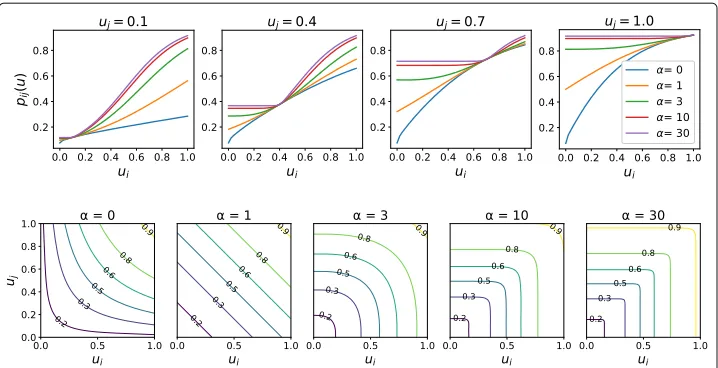
Now, givenu ∈ CR(n), the logistic core–periphery random model generates an edge from nodeito nodejwith independent probability given by
Pr(i→j)= 1
1+e−κα(ui,uj) =pij(u). (3)
Note that forα2≥α1≥0 we have
|xy| =κ0(x,y)≥κα1(x,y)≥κα2(x,y)≥κ∞(x,y)=max{|x|,|y|}.
Thus, for anyα ≥0, the probabilitypij(u)tends to be large if at least one of the nodesi andjhas a high core rank and this effect increases asαgrows, as shown by Fig.1.
Suppose we are given a network with the nodes in arbitrary order and wish to find the best core ranking assignment based on the logistic random model (3). From a maximum likelihood perspective, this corresponds to maximizing the log-likelihood
Lα(u)=
ij∈E
logpij(u)+
ij∈E/
log(1−pij(u)) (4)
among all possible u ∈ CR(n). In other words, assuming that the given network is a sample from the logistic core–periphery random model (3) with the node labels shuffled arbitrarily, this is most likely to be the correct reordering.
Fig. 1Probabilitypij(u
¯)for different values of the core scoresuj,uiand of the parameterα. Upper panel: pij(u
¯)as a function ofui, for different values ofujandα. Lower panel: contour plots ofpij(u¯)as a function ofui anduj, for different fixed values ofα
core quality functionfα. In fact, the following extension of Theorem 3.1 in (Tudisco and Higham2019) holds.
Theorem 1Let G be a directed unweighted graph. For anyα ≥0, a vectoru ∈CR(n) is solution of
max
u∈CR(n)Lα(u)
if and only if it is solution of
max
u∈CR(n)fα(u).
This equivalence provides further justification for the kernel optimization approach. It also suggests that the logistic core–periphery random model (3) is a useful resource for testing core–periphery detection algorithms in this directed setting.
We also note that a closely related generative random graph model for core–periphery networks was proposed in (Jia and Benson2018). That work focused on the undirected case and aimed to incorporate additionally available spatial information.
Core-periphery nonlinear operator
A study of the Hessian offα reveals that fα is neither convex nor concave in general. This makes the solution of (1) particularly challenging. However, here we show that this optimization problem can be re-cast in terms of the Perron eigenvector of a nonlinear operator. We then show how its solution is always achievable via a generalization of the classical power method from numerical linear algebra.
Givenα≥1, consider the nonlinear core-periphery operatorΦα:Rn→Rn, entrywise defined as follows
x→Φα(x)i= |xi|α−2xi n
j=1
Aij+Aji
κα(xi,xj)α−1
Givenp>1, we consider the following nonlinear eigenvalue problem forΦα
Φα(x)=λxp−1. (5)
One easily realizes thatΦα is linear if and only ifα = 1 in which case that operator degenerates into the map such thatΦ1(x)=din+dout, for any nonnegative vectorx≥0. In this setting it is easily seen that the only nonnegative solution of (5) isx =din+dout
withλ = 1 andp = 2. Combined with the discussion of the “Connection with degree and eigenvector centralities” section, this shows that for the caseα = 1 the unique nonnegative solution of the eigenvalue problem (5) coincides with the maximizer of (1). We can retrieve the same analogy for α → 0 andp = 1. In that case we have limα→0Φα(x)i = Φ0(x)i = √1xinj=1(Aij+Aji)√xjwhereas (5) becomesΦ0(x) = λ1. Arguing as in the “Connection with degree and eigenvector centralities” section, again, we deduce that forα=0 andp=1 a nonnegative solution of the eigenvalue problem (5) coincides with a maximizer of (1).
Whenα = 0, 1 the question of existence and uniqueness of a solution to (5) is less trivial. The following theorem gives a full answer and shows that the same one-to-one correspondence between (5) and (1) holds.
Theorem 2Letα≥0and p>max{1,α}. Then the eigenvalue problem (5) has a unique nonnegative solutionu≥ 0such thatup:=(|u1|p+ · · · + |un|p)1/p= 1which is also
the unique solution of (1), provided that · = · p. Moreoveruis positive if and only if
the network has no isolated nodes, i.e., all nodes have at least one outgoing or one incoming edge.
Note that, as no assumption on the connectedness of the graph is made, the eigenvector centrality, i.e., the nonnegative solution of (5) forα=0 andp=1, is not uniquely defined. Instead, Theorem2shows that the core–score assignment is always unique whenp >
max{1,α}andα≥0. The relevance of Theorem2is not only theoretical. In fact, it comes together with the following corollary which shows the global convergence touof a simple iterative scheme.
Corollary 1Given an initial guessu0 > 0and parametersα ≥0, p > max{1,α}and
q=p/(p−1), consider the following iterative method
vk+1=Φα(uk)
uk+1= vk+1q1−q|vk+1|q−2vk+1
, k=0, 1, 2, 3,. . .
Thenuk ≥0for all k≥0anduk−u =O
α−1 p−1
k
, i.e.,ukconverges to the unique
solutionu≥0of (1) and (5).
From Corollary1the choicepαappears to be attractive, since it leads an extremely rapid (linear) convergence rate. However, in choosing values forpandα, we must take account of two further issues.
1. As we argued in the “Core–periphery via functional kernel optimization” section, a larger value ofαgives a kernel that more closely matches the ideal of max{xi,xj}. 2. A larger value of pproduces a relaxed problem that is less likely to distinguish
between the nodes. (Note that in the extreme case of p = ∞, the constraint
x∞=1 allows for the obvious solutionx=1, which assigns the same score to all nodes).
Combining points 1 and 2 with Corollary1, we must compromise between a large param-eterαin the kernel and a not-too-large valuepfor the vector norm, while keepingp> α
to maintain convergence. In practice, we found that changing the value ofpdid not sig-nificantly affect the core–periphery structure output of the algorithm, which was instead governed by the value ofα. In our experiments we chosep = 2α andα = 10, as this produced good results with guaranteed fast convergence. Moreover, we observed that larger values ofα did not produce a noticeable change in the core–periphery structure identified.
Enron dataset
The Enron email network consists of 1,148,072 emails sent between 87,273 employees of Enron between 1999 and 2003. Nodes in the network are individual employees and weighted directed edges, with weights ranging from 1 to 3,904, count the number of emails sent from one employee to another. It is possible to send an email to oneself, and thus this network contains self–loops. Note that this network is not strongly (or even weakly) connected. The data has been collected from (Klimt and Yang2004).
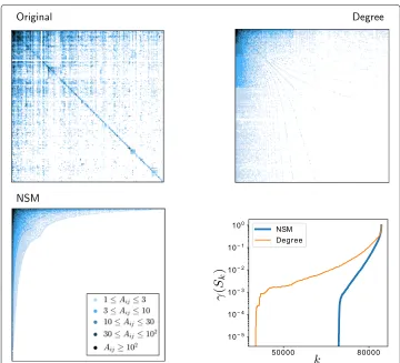
Three plots in Fig.2display the network by means of colored adjacency sparsity plots. Here, each nonzero entry in the adjacency matrix is shown with an intensity that corre-sponds to the edge weight (the darker the dot the larger the weight on the corresponding edge). These plots correspond to three different node labelings: the first one (top–left corner) is the original node labeling; the second plot (top–right corner) is the labeling, somewhat corresponding to a rich–club paradigm, obtained by re-ordering the nodes according to decreasing values of the overall degreedin+dout; the third one (bottom–left corner) is the labeling corresponding to decreasing values of the core–score computed with the NSM using parametersα=10 andp=20. This latter figure clearly shows that the Enron email dataset contains a strong core–periphery structure, which was less preva-lent initially. This is further confirmed by the core–periphery profile in the bottom–right plot, which shows the behavior of
γ (Sk)=
i,j∈SkAij
i∈Skd
in i +diout
Fig. 2Adjacency sparsity plots and core–periphery profile of the Enron email dataset. The two panels in the top and the panel in the bottom-left corner show the nonzero entries of the adjacency matrix of the network, with different color intensities for different edge weights, when the nodes are re-labeled in three different ways: the top-left panel corresponds to the original node labeling; the top-right panel is the labeling obtained by re–ordering the nodes according to decreasing values of the overall degree d
¯
in+d
¯
out; the bottom-left is
the labeling corresponding to decreasing values of the core–score computed with the proposed NSM. Finally, the bottom-right panel shows the persistence probabilityγ (Sk)as a function ofk, whenSkis the set
of thekmost peripheral nodes according to the degree vector (orange line) or the NSM (blue line)
periphery set. Thus a network has a strong core–periphery structure revealed by a core– score vector if the corresponding profileγ (Sk)takes small values askincreases from zero and then grows dramatically askcrosses some threshold value.
For undirected networks, the profileγ (Sk)was proposed in (Della Rossa et al.2013) as a means to visualize core-periphery structure. In this case,γ (Sk)coincides with the persistence probability of the setSk, i.e., the probability that a random walker who is currently in any of the nodes ofSk remains inSk at the next time step. For directed strongly connected networks, the persistence probability ofSk would instead be given byij∈S
kyiPij/
j∈Skyj, whereyis the stationary distribution of the random walk with
transition matrixPij=Aij/douti . However, as the Enron dataset we are considering is not connected,yis not well defined, and we computeγ (Sk)in its place.
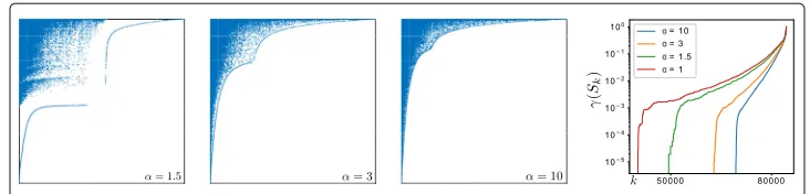
Fig. 3Adjacency matrix sparsity plots and core–periphery profiles corresponding to the relabeling obtained with the NSM and different values ofα
changing the value ofpdoes not effect the core–periphery structure output of the algo-rithm, small values ofαshow a weaker core–periphery structure, which is consistent with the fact that our model ideally works best whenα → ∞. However, in practiceα = 10 performs well and have observed that larger values ofα do not result in any significant change.
Since the network is not strongly connected, we do not show plots corresponding to the eigenvector centrality—this is not uniquely defined and, in our tests, different runs of Julia’sArpack.eigsgave rise to very different reorderings.
For this network the NSM with parametersα =10 andp=20 computed the solution to 9 digits of precision in less than 5 s on a standard i7 single core laptop, using Julia 1.0. Our code in both Matlab and Julia is available online at the addresshttps://github.com/ ftudisco/nonlinear-core-periphery.
Conclusion
Our main aim in this work was to show that the attractive properties of the nonlinear spectral method proposed in (Tudisco and Higham2019) can almost completely be trans-ferred to the directed, weighted and unconnected setting. In particular we show that for the core–periphery kernel quality function (1), proposed for example in (Rombach et al.2017; Tudisco and Higham2019), there is always a unique solution for α ≥ 0 and
p>max{1,α}, and this solution can be computed via a nonlinear spectral method when-ever it is feasible to form matrix-vector products based on the network weight matrix. The proposed method, which exploits an intriguing connection between optimization and eigenproblems, generalizes the classical power method in order to compute the global maximum of a highly nonconvex function; thus it may also be of interest in other machine learning contexts.
Appendix: Theorem proofs
ProofFirst note that, by adding and removingij∈Elog(1−pij(u)), the log likelihood (4) can be equivalently written as
Lα(u)=
ij∈E log
pij(u) 1−pij(u)
+
n
i,j=1
log(1−pij(u))=:S1(u)+S2(u).
Let us analyze the two termsS1andS2individually. Ifa= 1+e1−b, we have
a
1−a =
1 1+e−b
e−b
1+e−b
−1
=eb
S1(u)=
ij∈E log
pij(u) 1−pij(u)
=
ij∈E
κα(ui,uj)= n
i,j=1
Aijκα(ui,uj),
i.e.,S1(u) = fα(u). Now note that, ifu,v∈ CR(n)then there exists a permutationσ of
{1,. . .,n}such thatui=vσ(i)for alli. Therefore,
S2(u)= n
i,j=1 log
1 1+e−κα(ui,uj)
=
n
i,j=1 log
1 1+e−κα(vσ (i),vσ (j))
=S2(v),
which implies thatS2is constant on CR(n). ThusumaximizesLα(u) if and only if it
maximizesS1(u)and the proof is complete.
ProofThis proof is based on the proof of Theorem 4.5 in (Tudisco and Higham2019) and the lemmas therein proved. For convenience, let us denote byRn+the cone of vec-tors with nonnegative entries. Since we are interested in a nonnegative maximizer of
fα(x)constrained on the spherexp = 1, we can equivalently look for a maximizer of
fα(x/xp)on the whole cone of nonnegative vectorsRn+. Now, notice thatfαis positively 1-homogeneous, that isfα(ax)= afα(x)holds for any real numbera≥0. Therefore we can further change our problem into the global maximum onRn+ofg(x) = fα(x)/xp, without losing any generality. The critical point condition forgimplies the equivalence with the eigenvalue problem (5), i.e.,xis a stationary point forg if and only if it is such thatΦα(x) = λxp−1. Asp > 1, we can equivalently writeΦ(x)˜ = μx, withμ = λp−11
andΦ(x)˜ =Φα(x)
1
p−1. We now show that there can only be one nonnegativexsuch that xp=1 andΦ(x)˜ =μx.
To this end, note thatΦ(˜ x)≥0 for anyx≥0. Thus ifx≥0 andxp =1, thenμ >0 and we have
μ= μxp= ˜Φ(x)p= Φα(x)q−q 1,
whereqis such that 1/p+1/q = 1. Therefore anyx ≥0,xp = 1 solution of (5) is a fixed point of the map
:Rn+→Rn+, (x)= Φ(x)˜
˜Φ(x)p
= Φα(x)q−1 Φα(x)q−q 1
.
Letτ(x,y)= lnx−lny∞. Lemma 4.4 of (Tudisco and Higham2019) implies that
τ(x),(y)
τ(x,y) ≤
|α−1|
p−1 ,
for anyx,y∈Rn+. Asτ is a complete metric on the coneRn+(see, for example, (Lemmens and Nussbaum2012)), this shows thatis a contraction and thus it has a unique fixed point.
We conclude that, whenα > 0 andp > max{1,α}, the eigenvalue problem (5) has a unique nonnegative solutionu≥0 such thatup=1, which is also the unique solution of (1) when we choose · = · p. Note moreover that if we start with a positiveu0>0
and applyiteratively to giveuk+1=(uk)we obtainτ(uk+1,uk)≤
|α−1| p−1
k
Next we prove thatuhas a zero componentiif and only ifiis an isolated node, i.e., it has no incoming nor outgoing links. To this end, let+A⊆Rn+be the set of vectors
+
A = {x≥0 :xi=0 if and only ifiis isolated}.
Note that, equivalently,xi =0 forx∈+Aif and only ifAij+Aji =0 for allj=1,. . .,n. Now note that ifx∈+AthenΦα(x)∈+A. In fact, from its definition
Φα(x)i=xαi−1 n
j=1
Aij+Aji
κα(xi,xj)α−1
we see that, ifiis isolated,xi=0 and thusΦα(x)i=0, whereas ifxi>0, thenΦα(x)i>0 asκα(xi,xj) ≥ xi > 0 and there exists at least onej∗such thatAi,j∗+Aj∗,i > 0, which impliesΦα(x)i≥xiα−1(Ai,j∗+Aj∗,i)κα(xi,xj∗)1−α >0. Note that the same conclusion holds for any initial positive vector; that is,x >0 impliesΦα(x) ∈+A. Therefore the iterative method of Corollary1converges to a vector in+Afor any starting point, or, equivalently, any nonnegative solution of (5) must be in+A. Since there exists only one such solution, the proof is complete.
Acknowledgments
Not applicable.
Authors’ contributions
Both authors contributed to the problem formulation, algorithm design and analysis, and they co-wrote the manuscript. FT wrote the code for the computational experiments. Both authors read and approved the final manuscript.
Authors’ information
FT is a Reseach Assistant in the School of Mathematics at the University of Edinburgh (UK). DJH is Professor of Numerical Analysis in the School of Mathematics at the University of Edinburgh (UK).
Funding
The work of F.T. was supported by the European Union’s Horizon 2020 research and innovation programme under the Marie Skłodowska-Curie individual fellowship “MAGNET” No 744014. The work of D.J.H. is supported by the EPSRC/RCUK Established Career Fellowship EP/M00158X/1 and by the EPSRC Programme Grant EP/P020720/1.
Availability of data and materials
All data and code related to this work are publicly available at the GitHub online repositoryhttps://github.com/ftudisco/ nonlinear-core-periphery. The Enron dataset here used is also available athttp://konect.uni-koblenz.de/networks/enron.
Competing interests
The authors declare that they have no competing interests.
Received: 11 March 2019 Accepted: 22 July 2019
References
Baños R, Borge-Holthoefer J, Wang N, Moreno Y, González-Bailón S (2013) Diffusion dynamics with changing network composition. Entropy 15(11):4553–4568
Bascompte J, Jordano P, Melián CJ, Olesen JM (2003) The nested assembly of plant–animal mutualistic networks. Proc Natl Acad Sci 100(16):9383–9387
Bertozzi AL, Luo X, Stuart AM, Zygalakis KC (2018) Uncertainty quantification in the classification of high dimensional data. SIAM-ASA J Uncertain Quantif 6:568–595.https://doi.org/10.1137/17M1134214
Borgatti SP, Everett MG (2000) Models of core/periphery structures. Soc Netw 21:375–395
Csermely P, London A, Wu L-Y, Uzzi B (2013) Structure and dynamics of core/periphery networks. J Complex Netw 1(2):93–123
Cucuringu M, Rombach P, Lee SH, Porter MA (2016) Detection of core–periphery structure in networks using spectral methods and geodesic paths. Eur J Appl Math 27(6):846–887
Della Rossa F, Dercole F, Piccardi C (2013) Profiling core-periphery network structure by random walkers. Sci Rep 3:1467 Hoff PD, Raftery AE, Handcock MS (2002) Latent space approaches to social network analysis. J Am Stat Assoc
97(460):1090–1098
Horn RA, Johnson CR (1990) Matrix Analysis. Cambridge University Press, Cambridge
Jia J, Benson AR (2018) Random spatial network models with core-periphery structure. In: Proc. ACM International Conf. on Web Search and Data Mining (WSDM). ACM, New York
Klimt B, Yang Y (2004) The Enron corpus: A new dataset for email classification research. In: Proc. European Conf. on Machine Learning. Springer, Berlin. pp 217–226
Lemmens B, Nussbaum RD (2012) Nonlinear Perron-Frobenius Theory. Cambridge University Press, Cambridge Mondragón RJ (2016) Network partition via a bound of the spectral radius. J Complex Netw 5(4):513–526
Newman ME (2016) Equivalence between modularity optimization and maximum likelihood methods for community detection. Phys Rev E 94(5):052315
Newman MEJ (2011) Networks: an Introduction. Oxford University Press, Oxford
O’Connor L, Médard M, Feizi S (2015) Maximum likelihood latent space embedding of logistic random dot product graphs. arXiv preprint. arXiv:1510.00850
Rombach MP, Porter MA, Fowler JH, Mucha PJ (2014) Core-periphery structure in networks. SIAM J Appl Math 74:167–190 Rombach MP, Porter MA, Fowler JH, Mucha PJ (2017) Core-periphery structure in networks (revisited). SIAM Rev
59:619–646
Sandhu KS, Li G, Poh HM, Quek YLK, Sia YY, Peh SQ, Mulawadi FH, Lim J, Sikic M, Menghi F, et al. (2012) Large-scale functional organization of long-range chromatin interaction networks. Cell Rep 2(5):1207–1219
Schneider CM, Moreira AA, Andrade JS, Havlin S, Herrmann HJ (2011) Mitigation of malicious attacks on networks. Proc Natl Acad Sci 108(10):3838–3841
Tomasello MV, Napoletano M, Garas A, Schweitzer F (2017) The rise and fall of R & D networks. Ind Corp Chang 26(4):617–646
Tudisco F, Higham DJ (2019) A nonlinear spectral method for core-periphery detection in networks. SIAM J Math Data Sci 269–292.https://epubs.siam.org/toc/sjmdaq/1/2
Zhou S, Mondragón RJ (2004) The rich-club phenomenon in the internet topology. IEEE Commun Lett 8(3):180–182
Publisher’s Note