R E G U L A R A R T I C L E
Open Access
Capturing the fast-food landscape in
England using large-scale network analysis
Magda Baniukiewicz
1, Zachariah L. Dick
1and Philippe J. Giabbanelli
2**Correspondence: [email protected]
2Computer Science Department,
Furman University, Greenville, USA Full list of author information is available at the end of the article
Abstract
Fast-food outlets play a significant role in the nutrition of British children who get more food from such shops than the school canteen. To reduce young people’s access to fast-food meals during the school day, many British cities are implementing zoning policies. For instance, cities can create buffers around schools, and some have used 200 meters buffers while others used 400 meters. But how close is too close? Using the road network is needed to precisely computing the distance between fast-food outlets (for policies limiting the concentration), or fast-food outlets and the closest school (for policies using buffers). This estimates how much of the fast-food landscape could be affected by a policy, and complementary analyses of food utilization can later translate the estimate into changes on childhood nutrition and obesity. Network analyses of retail and urban forms are typically limited to the scale of a city. However, to design national zoning policies, we need to perform this analysis at a national scale. Our study is the first to perform a nation-wide analysis, by linking large datasets (e.g., all roads, fast-food outlets and schools) and performing the analysis over a high performance computing cluster. We found a strong spatial clustering of fast-food outlets (with 80% of outlets being within 120 of another outlet), but much less clustering for schools. Results depend on whether we use the road network on the Euclidean distance (i.e. ‘as the crow flies’): for instance, half of the fast-food outlets are found within 240 m of a school using an Euclidean distance, but only one-third at the same distance with the road network. Our findings are
consistent across levels of deprivation, which is important to set equitable national policies. In line with previous studies (at the city scale rather than national scale), we also examined the relation between centrality and outlets, as a potential target for policies, but we found no correlation when using closeness or betweenness centrality with either the Spearman or Pearson correlation methods.
Keywords: Network science; Obesity; Spatial networks; Zoning
1 Introduction
Road networks are one of the oldest forms of human-made infrastructure networks, pre-ceding power and telecommunication networks. Before network science became a pop-ular approach, geographers devoted several books to the analysis of road networks, in-cludingNetwork Analysis in Geographyfrom the late 1960s [1] and the influentialThe Seminal Logic of Spacein 1984 [2]. While some modern day cities may appear to have a grid-like pattern of roads, many road networks do not result from a central planning process but instead emerge over time as the result of an organic densification/exploration
process [3] thus creating structures far more complex than square grids. Despite being shaped by local geographical and socio-economical factors, road networks also exhibit structural commonalities across cities and countries. For example, Buhl and colleagues found similar average degrees [4] while Cardilloet al.reported a fractal dimension (per the box-counting method) in the narrow 1.7–2.00 range [5]. For a summary of these com-monalities, and a contextualization of findings among other spatial networks, we refer the reader to the review by Barthelemy [6].
Network science has been particularly interested in relating a network’sstructureto its
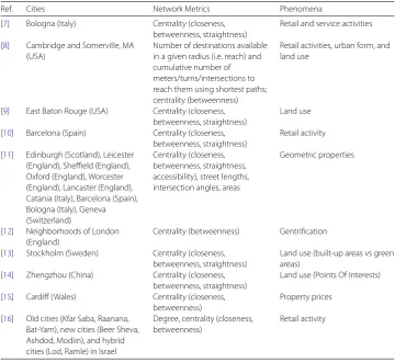
function. While there is a myriad of metrics, road networks are often analyzed with re-spect to betweenness centrality (since they are infrastructure networks and betweenness approximates traffic between all pairs of nodes) and closeness centrality (as a proxy to access). These metrics have been related to various phenomena, such as the presence of specific retail activities. In this paper, we focus on using the structure of road networks to understand the presence of fast-food outlets and its relation with the presence of schools. While analyses have been conducted on the structure of road networks at a large-scale [17,18], studying their relation with retail activities has predominantly been at the city level (Table1), which provides policymakers with information for a few selected cities but may not be sufficient for a national approach. Geographers and economists have also an-alyzed retail activities at a national level, but without using network-based metrics (e.g. shortest-paths calculations or centrality). For example, the geographical distribution of
Table 1 Network science studies investigating various structures in road networks (sorted by year)
Ref. Cities Network Metrics Phenomena
[7] Bologna (Italy) Centrality (closeness, betweenness, straightness)
Retail and service activities
[8] Cambridge and Somerville, MA (USA)
Number of destinations available in a given radius (i.e. reach) and cumulative number of meters/turns/intersections to reach them using shortest paths; centrality (betweenness)
Retail activities, urban form, and land use
[9] East Baton Rouge (USA) Centrality (closeness, betweenness, straightness)
Land use
[10] Barcelona (Spain) Centrality (closeness, betweenness, straightness)
Retail activity
[11] Edinburgh (Scotland), Leicester (England), Sheffield (England), Oxford (England), Worcester (England), Lancaster (England), Catania (Italy), Barcelona (Spain), Bologna (Italy), Geneva (Switzerland)
Centrality (closeness, betweenness, straightness, accessibility), street lengths, intersection angles, areas
Geometric properties
[12] Neighborhoods of London (England)
Centrality (betweenness) Gentrification
[13] Stockholm (Sweden) Centrality (closeness, betweenness, straightness)
Land use (built-up areas vs green areas)
[14] Zhengzhou (China) Centrality (closeness, betweenness, straightness)
Land use (Points Of Interests)
[15] Cardiff (Wales) Centrality (closeness, betweenness)
Property prices
[16] Old cities (Kfar Saba, Raanana, Bat-Yam), new cities (Beer Sheva, Ashdod, Modiin), and hybrid cities (Lod, Ramle) in Israel
Degree, centrality (closeness, betweenness)
retail outlets was investigated at the scale of Sweden using buffers [19], while food deserts were examined in rural U.S. counties using county-level data [20], and economic activities across countries were assessed by imposing a square grid [21]. In this paper, we present the first large-scale analysis of retail activities (focusing on fast-food outlets) using network methods across the whole of England.
Studying the geography of fast-food outlets at a detailed level (e.g. using network met-rics such as shortest-paths distances between outlets) over all of England is primarily mo-tivated by the current public health context. In the United Kingdom (UK), based on the National Child Measurement Programme 2013–2014, one third of children aged 10–11 and over a fifth of those aged 4–5 were overweight or obese [22]. The current policy land-scape in the UK emphasizes the role of eating patterns in achieving a healthy weight, and fast-food outlets have received particular attention. These outlets play a significant role in children’s nutrition: British secondary school children get more food from ‘fringe’ shops than from the school canteen [23]. In addition, even when there is a stay-on-site policy for lunch, the most popular time to buy food is after school [24]. This situation has led policy-makers to increasingly advocate for the regulation of fast-food outlets as part of an overall strategy of obesity prevention in school neighbourhoods. Between 2011 and 2014, four reports have called for a restriction of fast-food outlets around schools [25–28]. However, policies have so far differed widely in design as they can restrict fast-food outlets (i) in terms of clustering clustering (e.g. minimum distance between them) or (ii) respectively to schools (e.g. with a minimum distance from schools) [29]. In addition, the impact of fast-foods on obesity and food consumption varies over space, and particularly depend-ing on the deprivation of the area [30]. In this context, the principal contribution of the present work is to take a big data approach to propose the first investigation of fast-food activities based on road networks over an entire nation rather than on few select cities. Specifically, we conduct large-scale network analyses to:
(1) contribute to the evidence base for coordinated regulation at the level of England by analyzing distances (i) between fast-food outlets and (ii) between fast-food outlets and schools, across deprivation levels.
(2) investigate the relationship between centrality and the presence of fast-food outlets nation-wide, thus extending the scope of many previous studies employing network centrality mostly at the city-scale.
The remainder of this paper is divided into four sections. In Sect.2, we summarize the different geographical layers in England and the associated datasets used for this study. In particular, we contextualize these datasets with respect to previous studies of food outlets in England, and we explain the different steps to pre-process the datasets. Pre-processing includes assigning fast-food outlets and schools to roads, building the road network, and identifying the deprivation level of each road segment. Our analysis methods (including centrality metrics and their computation) are summarized in Sect.3, with results provided in Sect.4. Results are discussed in Sect.5in terms of their contribution to the evidence-base for public health in England, and regarding the potential of using large-scale analyses to inform regulations going forward.
2 Assembling a dataset
2.1 Overview
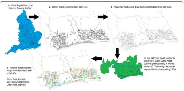
Figure 1Our five steps process to combine five datasets into one, specifying the location of fast-food outlets and schools within road as well as the level of deprivation.The high resolution version allows zooming to see detailed locations and deprivation levels within this sample LAD (Adur)
was accomplished in five steps, each involving the use of another dataset. We used a top-down process (Fig.1), starting with the whole of England (thus excluding Wales, Scotland, and Northern Ireland) and dividing it into coarse units. Steps 1 divides England in Lo-cal Authority Districts (LADs), specified in the 2016 boundary line dataset. In step 2, we added in the 2016 Ordnance Survey (OS) Open Roads containing 3,396,694 roads. Specif-ically, we found the roads that resided (either entirely or partially) within each LAD. In step 3, we retrieved the location of fast-food outlets and schools from the Points of In-terest (POI) data (PointX Database Right/Copyright 2016) obtained in January 2016. This dataset aggregates over 150 databases (in the ‘eating and drinking’ category) and has an accuracy ranging from 81% to 100% [30]. Locations for fast-food outlets were added to the street networks. At that stage, we had divided England into 327 LADs, each contain-ing a road network, with fast-food outlets and schools assigned to each road segment. Although studies differ on how they measure deprivation, or the specific relation being deprivation and childhood obesity, they have often found a correlation between either de-privation and childhood obesity, or dede-privation and the density of fast-food outlets (which also correlated with childhood obesity) [31–33]. Therefore, we also tracked deprivation using the official measure for small areas in England, the Index of Multiple Deprivation (IMD). This index takes into account employment, living environment, crime, health, ed-ucation, income, and housing [34]. Tracking this score took two additional steps, because it was provided in datasets using different geographical units.
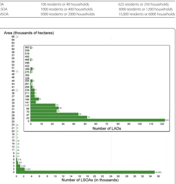
Table 2 Minimum and maximum values for each subdvision type in the UK
Subdivision Min value Max value
OA 100 residents or 40 households 625 residents or 250 households LSOA 1000 residents or 400 households 3000 residents or 1200 households MSOA 5000 residents or 2000 households 15,000 residents or 6000 households
Figure 2Distribution of sizes for LSOAs and LADs (inset), in thousands of hectares. The average LAD had 67,323±78,264 hectares, while the average LSOA had 561±1621 hectares
using them in anationalstudy (together with the whole road network) and conducting a detailednetworkanalysis are two of the hallmarks of the present study, in contrast with previous work (Table3).
In step 4, we used the latest (2011) census division of England into 34,753 LSOAs (which also included Wales). We removed Wales, and identified the LSOAs to which each road segment belonged. Finally, step 5 cross-referenced the LSOAs with the 2015 Indices of Multiple Deprivation dataset: since we knew the LSOA for each road, and the deprivation for each LSOA, we were able to assign a deprivation level for each road. The summary of datasets involved is provided in Table4.
Table 3 Key features of previous studies of fast-food outlets in the UK
Ref. Area Data Analysis
[37] Norfolk county
The location of food-related outlets was extracted from the Yellow Pages directory issued in six years (1990, 1992, 1996, 2000, 2003, 2008). Locations were overlaid onto the 2001 electoral ward boundaries for Norfolk (n= 205)
Repeated measures analysis of variance (RMANOVA)/multiple logistic regression model
[38] England and Scotland
The location of McDonald’s restaurants (n= 942) were obtained from the Yellow Pages directory and overlaid on 38,987 small areas: 6505 ‘Data zones’ in Scotland and 32,482 Super Output Areas in England
One-way analysis of variance
[30] Avon county
The location of outlets was extracted from the Ordnance Survey Points of Interest in Avon county
Geographically weighted regression
[35] Berkshire county
The location of outlets was obtained from six local councils, with analyses at the LSOA level
Cross-classified multi-level model with Markov chain Monte Carlo methods [36] North East
of England
The location of food-related outlets was extracted from the Yellow Pages directory, with analyses at the LSOA level
Correlation analysis, logistic multinomial regression, ANOVA
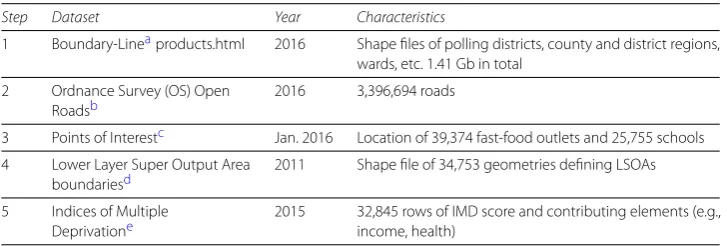
Table 4 Datasets combined for our study
Step Dataset Year Characteristics
1 Boundary-Lineaproducts.html 2016 Shape files of polling districts, county and district regions, wards, etc. 1.41 Gb in total
2 Ordnance Survey (OS) Open Roadsb
2016 3,396,694 roads
3 Points of Interestc Jan. 2016 Location of 39,374 fast-food outlets and 25,755 schools 4 Lower Layer Super Output Area
boundariesd
2011 Shape file of 34,753 geometries defining LSOAs
5 Indices of Multiple Deprivatione
2015 32,845 rows of IMD score and contributing elements (e.g., income, health)
https://osf.io/gn3f2/. Note that many of our spatial queries (e.g., to assess whether a road ‘fits’ within a LAD) require the open source libraryGeoToolsfor Java. As we do not own the data, links within Table4track data provenance.
2.2 Step 1: dividing England into local authority districts (LADs)
Our process starts by using the 326 shape files defining LADs, from the boundary-line dataset. Note that each result is not only a geometry defining the boundaries of the LAD, but a spatial object due to the use of coordinates. It also has a name, which later steps use to double-check linking across datasets.
Figure 3Roads are encoded in a shapefile as a series of segments. A segment links two points, specified as coordinates in easting and northing coordinates. Segments are created when a road has an intersection or turns
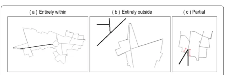
Figure 4Three cases regarding the relationship between a road and an area
2.3 Step 2: finding the road segments within each LAD
The input to step 2 consists of the output from step 1 (326 shape files for LADs) and the one shape file that defines roads as a series of segments, where new segments are made everytime a road bends or intersects with another road (Fig.3). The output is a road
network, divided across the LADs. To create this output, we need to (i) identify the (parts of ) roads that belong to each LAD, and (ii) convert roads from a shapefile format into a network. For the identification, we go through each LAD, and then through each road. The trivial cases are when the road falls entirely outside the LAD (discarded), or entirely within (assigned to the LAD). The one intermediate case is when apart of a road falls within a LAD (Fig.4). In this case, we divide the road in two segments: one segment for the LAD it belongs to (assigned to the LAD), and one remaining segment. Note that, while LADs do not overlap, some road segments may be at the border of two LADs. In this case, the segments are assigned to both LADs (i.e. duplicated). For the conversion, each road segment corresponds to one edge of our network, and each node stores the coordinates of the segment’s endpoints as in Fig.3. Note that our edges are not a one-to-one mapping of road segments in the road shape file, because some road segments may be sub-divided when they span two LADs.
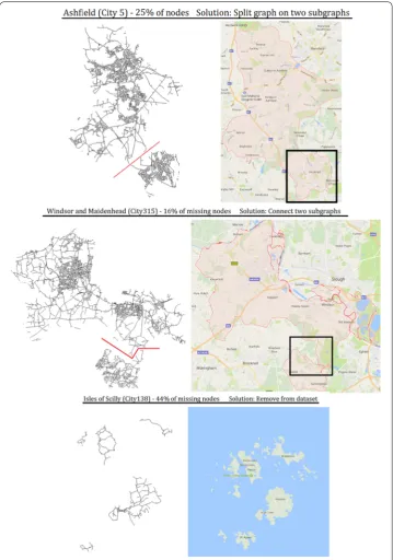
pre-processing. We found 6 LADs (less than 2% of the dataset) experiencing one of these two issues. This was mostly due to a misalignment between boundaries for governance (the LADs) and the transportation network (Fig.5). For example, one city could be in charge of two areas, but the only road to move between them was within the boundary of another city. The six cases were manually resolved. For Tewkesbury, Windsor and Maidenhead,
and Wyre, the small road fragment needed to connect the disjoint parts was re-assigned from the LAD where it fell (Cotswold and Gloucester, Bracknell Forest, and Fylde respec-tively). For Ashfield and North East Derbyshire, the parts that connected the ‘main’ city to a hamlet were far off, and we thus split each city into two LADs (one for the ‘main’ part and one for the hamlet). Finally, the Isles of Scilly contained roads over five discon-nected islands. Since our records indicate that the islands contained no schools and no fast-food outlets, we dropped this LAD from our dataset. We thus had 326 – 1 + 2 = 327 LADs.
2.4 Step 3: assigning schools and fast-food outlets to road segment
The input to this step consists of the road network divided across 327 LADs, and the Points of Interest (POI) data for schools and fast-food outlets. We obtained the complete POI data for England, and filtered it using the classification scheme version 3.1 to cate-gories 0018 (“Fast food and takeaway outlet”) and 31 (“Primary, secondary and tertiary education”) while noting that it does not include vocational schools (e.g., sailing schools, diving schools) or schools for outdoor pursuits (e.g., riding schools and equestrian cen-tres). Consequently, ‘schools’ at this step refers to all schools but vocational or outdoor-oriented, and ‘fast-food outlets’ refers to all of them regardless of whether they include a sitting area.
The data includes easting and northing coordinates, the postal code, and a district code. Several entries had missing information, such as incomplete postal codes or no district code. We discarded such incomplete entries, representing only 0.5% of the fast-food out-lets and 0.6% of the schools. For the remaining data, we assigned the entities to road seg-ments (i.e., edges of our network) in two steps: (i) identify the LAD based on the district code, and (ii) select the edge closest to the entity. A difficulty of step (i) is that the dis-trict code provides the name of a city, and not the name of a LAD. In most cases, the LAD had the same name as the city. However, for 36 cases, there was no LAD with the city’s name. This occured for LADs that represented counties, and had several cities (e.g., County Durham includes Durham, Derwentside, Sedgefield, Teesdale, etc.). All 36 cases were resolved manually, using Google Maps as geolocation service to find the city in Eng-land, and thus identify the LAD that it fits in. After completion of step (i), we knew the LAD for 99.5% of outlets and 99.4% of schools. For each entity within a LAD, we computed its distance to all road segments of that LAD, and we assigned it to the nearest segment (i.e. with minimum distance). The resulting network (Table5) has coordinates on the nodes,
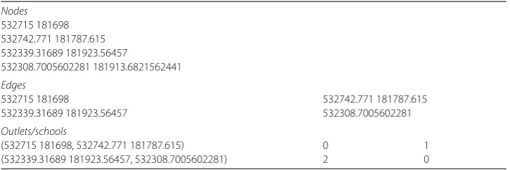
Table 5 Hypothetical example of data produced by step 3, showing a network where nodes have coordinates and edges count fast-food outlets as well as schools
Nodes
532715 181698 532742.771 181787.615 532339.31689 181923.56457
532308.7005602281 181913.6821562441
Edges
532715 181698 532742.771 181787.615
532339.31689 181923.56457 532308.7005602281
Outlets/schools
(532715 181698, 532742.771 181787.615) 0 1
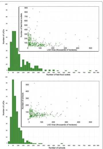
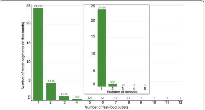
Figure 6Distribution of the number of fast-food outlets and schools (x-axis) across LADs (y-axis)
2.5 Step 4: identifying the lower layer super output area (LSOA) for each road segment
The LSOA contains statistical information. Identifying the LSOA of a road segment thus provides access to the deprivation level of this road segment. We started by excluding 5.63% of the LSOAs from the dataset because they were entirely outside of England, which is the focus of this work. Then, we identified the LSOA to which each road segment be-longed. Because LSOAs were not designed to match the transportation network, we had to operate in the same way as in step 2: segments entirely within an LSOA were assigned to it, while thosepartiallywithin the LSOA were further split. While LSOAs do not over-lap, we also noted that several road segments were exactly at the boundary of two LSOAs (53,459 segments or≈0.8%of the data), and we assigned them to both (i.e., a given edge has either one or two LSOAs).
This process resulted in a final network size of 6,549,676 edges and 6,102,863 nodes. This leads to an extremely low network density (≈3.51e–5), which we expect as a node is most frequently connected to two edges (since a road is stored as a series of lines) and cannot be connected to many others given the practical limitation on the number of roads that can intersect. When outlets were present on a street segment, there were on average 1.28±0.69 outlets. Similarly, when schools were present on a street segment, there were on average 1.03±0.20 schools. The distribution of schools and outlets per street segment is shown in Fig.7.
As this is the last step that affects the existence of an edge, we also finalized spatial infor-mation about each edge at this step by computing the edge’s length (based on the Euclidean distance between its two endpoints). Computing the distance was necessary to later an-swer questions such as howfarschools can be from fast-food outlets. The average edge had a length of 60±70 m, with the large standard deviation due to the simultaneous pres-ence of long non-intersecting straight roads as well as extremely small segments (e.g. for tiny portions of roads spanning two LADs, or a road with a strong curvature approximated by many small lines).
2.6 Step 5: adding the deprivation level of each road segment via its LSOA The Index of Multiple Deprivation (IMD), commonly refered to as ‘deprivation level’ here, is a floating-point number assigned to each LSOA. When a road segment had a single LSOA, we thus assigned it the deprivation level of its LSOA. For boundary roads assigned to two LSOAs, we could not assume that their deprivation would be more like one LSOA or the other, and thus we assigned them the average deprivation level of the two LSOAs. As in previous analyses of the fast-food outlets in England with respect to deprivation [38], we simplified the (continuous) deprivation level into tertiles. The first tertile contains deprivation levels up to 11.92 (included), the second tertile contains deprivation levels from 11.92 (excluded) to 24.845 (included), and the third tertile contains deprivation levels strictly greater than 24.845. The amount of LSOAs within each tertile could not be exactly the same (as the total was not dividable by three), hence there are 10,947 LSOAs in the first two tertiles and 10,949 LSOAs in the third tertile.
3 Analytical methods
3.1 Overview
The following two sub-sections detail why, and how we computed our results from the network assembled in the previous section. Some notation will be used throughout this section, and is introduced here. We denote a graphG= (V,E) as formed of a node setV
and an edge setE. The number of nodes and edges in the graph is denoted by|E|=mand |V|=nrespectively. The ‘cost’ of an algorithm will be expressed in the worst-case, that is, as the peak resources that it needs to complete. Resources are divided into time (i.e. time complexity) and space (i.e. space complexity). The worst-case complexity is expressed using theOnotation, showing how either the running time or space requirements grow as a function of mandn. For example, a space ofO(m) says that we need to store ‘in the order’ of the number of edges for an algorithm (thus omitting constants). For larger networks such as ours, acceptable costs rarely exceed quadratic forms: for instance,O(n2)
maybe feasible, butO(n3) may exceed available resources. When computing distances, we chose algorithms that provide exact answers at costs less than quadratic. When computing centralities, we opted for approximation algorithms given the high cost of the exact ones. Computations were performed on the shared High Performance Cluster (HPC) Gaea at Northern Illinois University, typically using 5 nodes (each equipped with 2 Intel X5650 processors and 72 Gb RAM). Our scripts for analysis are available within the ‘Analysis’ folder athttps://osf.io/gn3f2/.
3.2 Computing shortest-path distances
are made on a best-guess basis, reflected by a wide array of values. For instance, Islington Council set a 200 meters buffer between schools and fast-food outlets, while others used a 400 meters buffer (Warrington Borough Council, City of Bradford, Barking and Dagen-ham, Solihull council) [39–43]. Similarly, the clustering was set to having no more than 10% of units in an area for Gateshead Council, whereas Barking and Dagenham used a 5% limit, and Solihull imposed a 15% limit. Target areas also varied, with some using zoning to control town centers whereas others targeted specific demographics (e.g., Gateshead Council imposed restrictions in wards where more than 10% of year 6 pupils were obese) [39,40,44]. Consequently, a major contribution of our work is to compute the distances used in both policy levers. That is, we compute the shortest distances (i) between fast-food outlets, and (ii) between fast-food outlets and schools.
The genericsolution to compute shortest-path distances between two objects (i.e., a fast-food outlet and another outlet or school) is typically the Bellman–Ford algorithm those time complexity isO(mn). In networks exhibiting desirable properties, more spe-cific solutions can be identified. In our network, edges have a strictly positiveweight, rep-resenting the length of the corresponding road segment. In this situation, Dijkstra’s algo-rithm is faster due to a time complexity ofO(m+nlogn). While there exists an optimal
O(n) algorithm for planar networks [45] (i.e. which can be drawn without two overlap-ping edges), the British road network does not satisfy this constraint due to the pres-ence of overpasses (called flyover) including stack interchanges (when roads are above each other on multiple levels). We note that this problem does not affect all LADs: as of 2017,http://www.cbrd.co.uk/estimated that there were less than 30 stack interchanges in the UK. Computations may thus be optimized by processing planar LADs differently than non-planar ones. However, to run distributed computations on the HPC facility, we ensured that the same version of the code was used for all inputs. Consequently, we implemented Dijkstra’s algorithm, and results were computed within approximately 42 hours.
3.3 Relating the presence of fast-food outlets to centralities
for each LAD independently, and then results are combined across the LADs. This en-sures that there is no contagion effect: the centrality of a street segment in a city depends only on the topology of this city, rather than on the city’s position in the country. In other words, by splitting the whole network into LADs and measuring centrality within each LAD, our results are not influenced by whether a city is close to the sea or border (which may lower the centrality of its streets) or situated around the middle of the country (which may inflate its centrality).
Box 1.Process to relate node centrality and the density of fast-food outlets. (1) Remove nodes whose centrality would be zero.
(2) Approximate the centrality of the nodes. (3) Transform the centrality into a ranking of nodes.
(4) Compute the number of fast-food outlets nearest to each node. (5) Correlate (3) and (4).
Intuitively, the betweenness centrality of a nodexis the fraction of shortest paths be-tween pairs of nodes in a network that pass throughx. The closeness centrality ofxis the inverse of the distance required, fromx, to reach all other nodes through shortest paths. Betweenness and closeness centralities are formally stated in the two definitions below. Note that they are both centralityindices. For instance, for two elementsxandy, if the centralityc(x) is at least as much asc(y), then we conclude thatxis at least as central asy. As stated by Koschutzkiet al., “in general, the difference or ratio of two centrality val-ues cannot be interpreted as a quantification of how much more central one element is than the other” [50]. Given that our goal is to correlate the centrality with the presence of urban elements, we do not want the correlation to be biased by wrongly using relative differences in centrality. After computing the centrality of all nodes, we thus normalize it by transforming it into a ranking.
Definition 1 Letσst(v) denote the number of shortest paths between two nodess,t∈V
that containv∈V. Then, thebetweenness centralityof a nodeu∈Vis given by [50]:
cB(u) =
σst(v)
σst
. (1)
Definition 2 Letd(u,v) denote the shortest-path distance between two nodesu,v∈V. Then, thecloseness centralityof a nodeu∈Vis given by [50]:
cC(u) =
1
v∈Vd(u,v)
. (2)
Figure 8Nodes with a single edge are easy to identify, and removed before computing the betweenness centrality. This example in Adur City shows how 12 nodes (red circles) can be removed, as no path goes through them
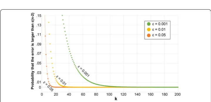
Figure 9Probability that the error exceeds a target (depending on) for different number of pivotsk. Computations were performed for Cornwall
go through them (Fig.8). Similarly, for closeness, we excluded unreachable nodes (since their distance to others would be infinite and their closeness tend to 0). This approach removed approximately 14% of nodes when computing betweenness, and less than 1% of nodes for closeness. We thus had to use a second step, in which we employ Eppstein and Wang’s fast approximation algorithm for betweenness and closeness [51]. The algorithm randomly selectskpivots, and provides the probability that estimation errors are greater than×(n– 2). A higherkor a lowerwould lead to more accurate results at the expense of performing more computations. We thus have to identify suitable values of the param-eterskand, while noting that these choices are interdependent (Fig.9). We setto a 5% error margin, and we performed a parameter sweep across all 327 LADs and values ofk
(from 1 to 1000). We identifiedk= 109 as providing a good level of accuracy while keeping computational time small (Fig.10).
betwen-Figure 10 After settingto 5%, approximation errors depend on the number of pivotsk(y-axis) and the number of nodesn, which varies across cities (x-axis). We found that the choice of city did not have a noticeable impact. Approximation error became small in the range 100–150 (top), and we chosek= 109 (bottom; framed). Due to the wide range of values, note that scales (i.e. colormaps) are different
ness and closeness. Correlation values range from –1 (perfect negative correlation) to 1 (perfect positive correlation). Correlation values were computed using both the Spearman and the Pearson correlation methods, to assess whether there was a monotonic (for Spear-man) or linear (for Pearson) relationship between the presence of fast-food outlets and the centrality metric.
4 Results
The datasets produced by our analysis (previous section) are available within the ‘Results’ folder athttps://osf.io/gn3f2/. We computed the distributions of distances between fast-food outlets and (i) the nearest fast-fast-food outlet, as well as (ii) the nearest school. Based on these distributions (Fig.11), we can make the following observations:
– Fast-food outlets are very strongly clustered. Most of them are located either on the same spot or within a few dozen meters (60% of the data falls within 0 to 60 meters). Using a 120 m buffer suffices to capture almost 80% of the outlets.
– While outlets are strongly clustered around each other, they are much less clustered around schools. Less than 5% of outlets are found within 60 meters of a school (compared to 60% with respect to other outlets), and less than 20% of outlets are found within 120 m of a school (compared to 80% with respect to other outlets). – The widest buffer of 600 m around a school would capture over 80% of existing
outlets, while the other classic buffer of 420 m would capture about 65%. This shows that doubling the buffer does not double the number of outlets included.
differ-Figure 11 Distribution of distances (in meters) between outlets (a) as well as between outlets and schools (b). Thea-axis goes up to 600 m as it is the largest value encountered in current zoning policies regarding fast-food outlets and schools in England.An expanded version of the figure also using Euclidean distances is available onhttps://osf.io/gn3f2/
Figure 12 Fit between the analysis output (transformed from discrete to continuous) using a log-log plot (a) and a linear-linear plot (b), for a medium level of deprivation, for distances between fast-food outlets and schools.An expanded version of the figure showing all four combinations of linear and logarithmic scales is available onhttps://osf.io/gn3f2/
Table 6 Fits across levels of deprivation and scaling of the axes
Deprivation Distance scale (x-axis) Fraction of outlets scale (y-axis) p-value R2of a linear fit
Overall linear linear <0.0001 0.996989
log 0.776541
log linear 0.810363
log 0.993964
Tertile 1 linear linear 0.99789
log 0.786763
log linear 0.828365
log 0.991716
Tertile 2 linear linear 0.996447
log 0.782838
log linear 0.795886
log 0.994874
Tertile 3 linear linear 0.996617
log 0.769842
log linear 0.813284
log 0.992019
Figure 13 Distribution of Pearson correlations between the density of fast-food outlets and (a) betweenness centrality or (b) closeness centrality
The correlation between centrality and the presence of fast-food outlets is shown in Fig.13for the Pearson correlation, and Fig.14for the Spearman correlation. We observe that almost all of the data falls within the range [–0.1, 0.1] in which we conclude to the absence of a correlation. While three points fall outside this range, they are still at a very low level of correlation and may be outliers.
5 Discussion
Figure 14 Distribution of Spearman between the density of fast-food outlets and (a) betweenness centrality or (b) closeness centrality
Our first research question was to identify the distances between fast-food outlets and (i) other outlets as well as (ii) schools. This was motivated by the pressing need for a na-tional evidence base to either (i) increase distances between fast-food outlets by limiting clustering, or (ii) create a buffer around schools. The 2011 guidance from the National Institute for Health and Clinical Excellence recommended that local authorities regulate the number of fast-foods in specific areas, such as within walking distance of school [25]. The 2013 Academy of Medical Royal Colleges’ report advocated to “reduce the proximity of fast food outlets to schools, colleges, leisure centres and other places where children gather” [55]. However, neither could say exactly by which distance to reduce it, and what number of outlets would be affected, as this analysis was not previously available. Follow-ing these recommendations, several local authorities have started to use plannFollow-ing as a tool to address childhood obesity. As summarized by Peter Wright, an emerging view is that improving nutritional quality
“is not an issue that will be satisfactorily resolved by voluntary improvement, educa-tion, advice or any other “easy” intervention. Without political will and a determina-tion to limit the proliferadetermina-tion of takeaway food businesses we are unlikely to make any meaningful impact on the impact of poor diet on significant parts of the population.”
Peter Wright, Gateshead Council, Centre for Diet and Activity Research (CEDAR), ‘Neighbourhood food environments, diet and health: research policy meeting’, Nov. 4th 2014, Cambridge, UK.
This illustrates the two unknowns: what distance should we use, and how many fast-food outlets would it capture? The Takeaways Toolkit, considered to be one of the reference documents to assist with designing regulations, has previously emphasized the need for more evidence since such planning measures “have not yet been evaluated, and the im-pact on obesity and other health issues remains unknown”. This study contributes to the creation of robust evidence through our national-scale analysis of distances. We found strong spatial clusters of fast-food outlets (Fig.11(a)): most fast-food outlets were within a few dozen meters from each other, and 80% of them were within 120 meters. However, clusters around schools were significantly weaker (Fig.11(b)): less than 5% of outlets were within a few dozen meters from schools, and going as far as 120 meters captures less than 20% of them (compared to 80% when using other outlets as referential). This finding is in contrast to previous studies finding strong clusters around schools. This difference may be explained partially by context, as previous analyses were conducted in Scotland, New Zealand, or the United States instead of the United Kingdom [56–58]. Our data can also inform authorities having implemented buffers around schools about the average fraction of outlets that may be captured: the 200 meters buffer for Islington Council [43] may im-pact a third of the outlets (based on national averages), while the 400 meters used by others may impact half of the outlets [39–41,43]. This suggests that increasing the distances be-tween fast-food outlets may create more disruptive changes in the foodscape. However, like many upstream interventions, being disruptive can be both an opportunity (to avoid concentrated obesogenic environments) and a challenge (as many actors are concerned and a high political capital may be needed to enact such changes). Our last contribution regarding fast-food outlets and schools is to examine their relation across levels of depri-vation. We found that a scaling law was most likely to govern the relationship between distances from schools and the fraction of fast-food outlets. The underlying explanation for this scaling law would need to be explored in a follow-up study, for instance by using the concept offractal dimensionof a city. As shown by the comprehensive study of Ribeiro
et al.[52], the concept of fractal dimension is related to urban metrics of infrastructure (e.g., using the number of fast-food outlets as infrastructure variable) and the decaying influence of one node over another.
Our second research question was to investigate the relationship between network cen-trality and the density of fast-food outlets, thus taking previous local studies (Table1) to a national scale. While previous studies found strong correlations between centrality and economic activities (R2= 0.61 [10], orR2= 0.651 [14]), we found no correlation using ei-ther Spearman or Pearson methods: the correlation was close to 0 for 324 out of 327 areas, and only marginally beyond –0.1 or 0.1 for 3 areas (Figs.13and14). This suggests that, either at the national scale or at the scale of our areas, closeness or betweenness centrality were not a sufficiently strong factor to explain the location of outlets.
differentiation from the competition helps to avoid price rivalry and increase chances for monopoly rents. Consequently, not all stores may want to occupy a position with a high flow (betweenness centrality) or that easily reaches other destinations (closeness central-ity). In addition, separation increases market coverage, which has historically been shown to play a role when travel costs are important to customers [60] or if demand changes over time [61]. Centrality may thus have to be conceptualized as a competitive process, which is captured by a few centrality indices such as the centroid [50]. However, studies on street networks and the presence of retail activities predominantly use centrality indices from the Multiple Centrality Assessment (MCA) method created by Porta and colleagues [7], which includes betweenness and closeness centrality but does not encompass the centroid method or competitive centralities. While the application of the centroid method would be an interesting alternative, it still may not fully capture the presence of fast-food outlets as their location is driven by a balance of competition and attraction (e.g., to influence customers’ ability to remember locations and contrast offers [59]).
While our study combines large datasets from the national mapping agency with other governmental sources, there are nonetheless limitations to this work. The first and main limitation is that our work is primarily of benefit to quantify economic impacts, whereas the translation into health outcomes would require a simulation. That is, our work pro-vides estimates about how much of the food landscape may be impacted given current distances. This is the exposure to foods. Our study does not directly explain what health consequences may be obtained by a policy. This requires understanding how changing the exposure to foods would impact their utilization by children, and linking the change in diet to a change in obesity. An agent-based model could build on our work to simulate how agents (i.e. children) utilize the food environment [62], which would require detailed datasets on the food environment and childhood obesity such as the Child Obesity and Excess Weight dataset.f
make inferences aboutcausation. Our next study will focus on causation, examining how different factors may successfully replicate the location of fast-food outlets.
Acknowledgements
PJG would like to thank members of the Global Obesity Prevention Center (GOPC) for feedback on the overall project, including Dr Bruce Lee, Dr Tom Glass, and Dr Joel Gittelsohn. MB is also grateful for financial assistance from the Institute for Pure & Applied Mathematics (University of California in Los Angeles) to attend the workshop on Multiscale
Data-driven Models, and from the University of Alabama at Birmingham to attend a course on the Mathematical Sciences in Obesity Research; both have contributed to shaping the ideas presented in this paper. All computations were performed through the Center for Research Computing and Data at Northern Illinois University, with assistance from John Winans. Finally, both authors are indebted to Eva Maguire at the University of Cambridge for sharing her expertise on fast-food outlets in England.
Funding
Research reported in this article was supported by the Global Obesity Prevention Center (GOPC) at Johns Hopkins (project “Assessing the impact of zoning policies on fast-foods around schools”—Dr Giabbanelli PI), and the Eunice Kennedy Shriver National Institute of Child Health and Human Development (NICHD) and the Office of The Director, National Institutes of Health (OD) under award number U54HD070725. The content is solely the responsibility of authors and does not necessarily represent the official views of the National Institute of Health.
Abbreviations
IMD, Index of Multiple Deprivation, which takes into account multiple variables such as takes employment and education; LAD, Local Authority District, a division of the UK based on local governance; LSOA, Lower layer Super Output Areas, a division of the UK based on census data; HPC, High Performance Cluster, the equipment used to perform our computationally intensive analysis; POI, Points of Interest, database for this study; SPD, Supplementary Planning Document, used by local governments to enact planning policies; UK, United Kingdom, focal country for this study.
Availability of data and materials
The datasets supporting the conclusions of this article are available through national sources as listed in Table4. Our pre-processing scripts, analysis scripts, and results are hosted on the Open Science Framework athttps://osf.io/gn3f2/.
Competing interests
The authors declare that they have no competing interests.
Authors’ contributions
Authors contributed with the order they appear. All authors read and approved the final manuscript.
Authors’ information
MB graduated from Northern Illinois University with an MS in computer science. Her thesis, supervised by PJG, focused on analyzing and simulating complex social systems. Her work on obesity recently appeared as a chapter inAdvanced Data Analytics in Health. ZLD is an undergraduate student at Northern Illinois University in computer science. He is supervised by PJG, and aims to take this research further through the use of machine learning. PJG was previously an assistant professor at Northern Illinois University, and is now an assistant professor at Furman University. He has authored close to 60 articles with a focus on modeling and analyzing health behaviors.
Author details
1Department of Computer Science, Northern Illinois University, DeKalb, USA.2Computer Science Department, Furman
University, Greenville, USA.
Endnotes
a https://www.ordnancesurvey.co.uk/opendatadownload/. b https://www.ordnancesurvey.co.uk/opendatadownload/.
c https://www.ordnancesurvey.co.uk/business-and-government/products/points-of-interest.html. d https://data.gov.uk/dataset/lower_layer_super_output_area_lsoa_boundaries.
e https://www.gov.uk/government/uploads/system/uploads/attachment_data/file/467774/File_7_ID_2015_All_
ranks_deciles_and_scores_for_the_Indices_of_Deprivation__and_population_denominators.csv/preview. f https://data.gov.uk/dataset/child-obesity-and-excess-weight.
Publisher’s Note
Springer Nature remains neutral with regard to jurisdictional claims in published maps and institutional affiliations.
Received: 16 January 2018 Accepted: 7 October 2018 References
1. Haggett P, Chorley R (1969) Network analysis in geography. Arnold, London
4. Buhl J, Gautrais J, Reeves N, Sole R, Valverde R, Kuntz P, Theraulaz G (2006) Eur Phys J B 49:513 5. Cardillo A, Scellato S, Latora V, Porta S (2006) Phys Rev E 73:066107
6. Barthelemy M (2011) Phys Rep 499:1
7. Porta S, Strano E, Iacoviello V, Messora R, Latora V, Cardillo A, Wang F, Scellato S (2009) Environ Plan B, Plan Des 36(3):450
8. Sevtsuk A (2010) Path and place: a study of urban geometry and retail activity in Cambridge and Somerville, MA. http://dspace.mit.edu/handle/1721.1/62034
9. Wang F, Antipova A, Porta S (2011) J Transp Geogr 19(2):285
10. Porta S, Latora V, Wang F, Rueda S, Strano E, Scellato S, Cardillo A, Belli E, Càrdenas F, Cormenzana B, Latora L (2012) Urban Stud 49(7):1471
11. Strano E, Viana M, da Fontoura Costa L, Cardillo A, Porta S, Latora V (2013) Environ Plan B, Plan Des 40(6):1071 12. Venerandi A, Zanella M, Romice O, Porta S The form of gentrification.https://arxiv.org/abs/1411.2984 13. Rui Y, Ban Y (2014) Int J Geogr Inf Sci 28(7):1425
14. Cui C, Han Z (2015) Spatial data mining and geographical knowledge services (ICSDM). 2015 2nd IEEE International Conference on, pp 88–92
15. Xiao Y, Orford S, Webster CJ (2016) Environ Plan B, Plan Des 43(1):108 16. Omer I, Goldblatt R (2016) Urban Geogr 37(4):629
17. Arcaute E, Molinero C, Hatna E, Murcio R, Vargas-Ruiz C, Masucci AP, Batty M (2016) R Soc Open Sci 3(4) 18. Molinero C, Murcio R, Arcaute E (2017) Sci Rep 4312
19. Amcoff J (2016) Int Rev Retail Distrib Consum Res 26(3)
20. Blanchard TC, Matthews TL (2007) Remaking the North American food system: strategies for sustainability 21. Ghosh T, Powell RL, Elvidge CD, Baugh KE, Sutton PC, Anderson S (2010) Open Geogr J 3(1)
22. Health, S.C.I. Center (2015). National child measurement program—England, 2013–2014.www.hscic.gov.uk/ncmp 23. Sinclair S, Winkler J (2008) Nutrition policy unit (London Metropolitan University)
24. Sinclair S, Winkler J (2009) Nutrition policy unit (London Metropolitan University)
25. N.I. for Health, C.E. (NICE) (2011) Public health guideline 35.https://www.nice.org.uk/guidance/ph35
26. A. of Royal Medical Colleges (2013) Measuring up: The medical profession’s prescription for the nation’s obesity crisis 27. 2020Health. Careless eating costs lives (2014).
http://www.2020health.org/2020health/Publications/Publications-2014/CarelessEatingCostsLives.html
28. L.H. Commission (2014). Better health for London. http://www.londonhealthcommission.org.uk/better-health-for-london/
29. U.H.C. Network (2011). Information booklet.http://www.healthycities.org.uk/UK_Healthy_Cities_Network_Brochure. pdf
30. Fraser LK, Clarke GP, Cade JE, Edwards KL (2012) Am J Prev Med 42(5):e77.http://www.sciencedirect.com/science/ article/pii/S0749379712001298. Online; accessed 22-September-2016
31. Kinra S, Nelder RP, Lewendon GJ (2000) J Epidemiol Community Health 54(6):456 32. Edwards KL, Clarke GP, Ransley JK, Cade J (2010) J Epidemiol Community Health 64(3):194 33. Fraser LK, Edwards KL (2010) Health Place 16(6):1124
34. Noble M, Wright G, Dibben C, Smith G, McLennan M, Anttila C, Barnes H, Mokhtar C, Noble S, Avenell D (2014) The English indices of deprivation 2004: Report to the office of the deputy prime minister
35. Williams J, Scarborough P, Townsend N, Matthews A, Burgoine T, Mumtaz L, Rayner M (2015) PLoS ONE 10(7):e0132930.http://journals.plos.org/plosone/article?id=10.1371/journal.pone.0132930. Online; accessed 22-September-2016
36. Burgoine T, Alvanides S, Lake AA (2011) Health Place 17(3):738.http://www.sciencedirect.com/science/article/pii/ S1353829211000190. Online; accessed 22-September-2016
37. Cummins SC, McKay L, MacIntyre S (2005) Am J Prev Med 29(4):308.http://www.sciencedirect.com/science/article/ pii/S0749379705002564. Online; accessed 22-September-2016
38. Maguire E, Burgoine T, Monsivais P (2015) Health Place 33:142.http://www.sciencedirect.com/science/article/pii/ S1353829215000325. Online; accessed 22-September-2016
39. Council—London Borough of Barking & Dagenham (2010) Saturation point—addressing the health impact of hot food takeaways. https://www.lbbd.gov.uk/wp-content/uploads/2014/10/Saturation-Point-SPD-Addressing-the-Health-Impacts-of-Hot-Food-Takeaway.pdf. Accessed: March 13, 2017
40. Charlene J (2014) Hot food takeaway supplementary planning document draft for consultation.http://www.solihull. gov.uk/Portals/0/Planning/LDF/Draft_HFT_SPD.pdf. Accessed: March 13, 2017
41. Council—City of Brandford (2014) The hot food takeaway supplementary planning document.https://www. bradford.gov.uk/media/3039/hotfoodtakeawaysupplementaryplanningdocument.pdf. Accessed: March 13, 2017 42. Hot food takeaways supplementary planning document (2014)https://www.warrington.gov.uk/download/
downloads/id/8680/hot_food_takeaway_spd_april_2014.pdf. Accessed: March 13, 2017
43. Location and concentration of uses supplementary planning document (2016)https://www.islington.gov.uk//~/ media/sharepoint-lists/public-records/planningandbuildingcontrol/publicity/publicconsultation/20162017/ 20160505locationandconcentrationofusesspdadoptedapril2016. Accessed: March 13, 2017
44. Willumsen T (2016) Hot food takeaway supplementary planning document.http://www.gateshead.gov.uk/ DocumentLibrary/Building/PlanningPolicy/SPD/Hot-Food-Takeaway-SPD-2015.pdf. Accessed: March 13, 2017 45. Henzinger MR, Klein P, Rao S, Subramanian S (1997) J Comput Syst Sci 55(1):3
46. Barthélemy M (2004) Eur Phys J B 38(2):163 47. Holme P (2003) Adv Complex Syst 06(02):163
48. Zhang D, Giabbanelli PJ, Arah OA, Zimmerman FJ (2014) Am J Publ Health 104(7):1217
49. Aggarwal A, Cook AJ, Jiao J, Seguin RA, Moudon AV, Hurvitz PM, Drewnowski A (2014) Am J Publ Health 104(5):917 50. Koschützki D, Lehmann KA, Peeters L, Richter S, Tenfelde-Podehl D, Zlotowski O (2005) Centrality indices Springer,
Berlin, pp 16–61
52. Ribeiro FL, Meirelles J, Ferreira FF, Neto CR (2017) R Soc Open Sci 4(3):160926 53. Caglioni M, Giovanni R (2004) Cybergeo: Eur J Geogr
54. Batty M, Longley PA (1994) Fractal cities: a geometry of form and function. Academic press, San Diego
55. A. of Royal Medical Colleges (2013) Measuring up: The medical profession’s prescription for the nation’s obesity crisis 56. Austin S, Melly S, Sanches B, Patel A, Buka S, Gortmaker S (2005) Am J Publ Health 95(9):1575.
http://www.ncbi.nlm.nih.gov/pmc/articles/PMC1449400/. Online; accessed 22-September-2016 57. Day PL, Pearce J (2011) Am J Prev Med 40(2):113.
http://www.sciencedirect.com/science/article/pii/S0749379710006112. Online; accessed 22-September-2016 58. Ellaway A, Macdonald L, Lamb K, Thornton L, Day P, Pearce J (2012) Health Place 18(6):1335
59. Krider RE, Putler DS (2013) Geogr Anal 45(2):123
60. d’Aspremont C, Gabszewicz JJ, Thisse JF (1979) Econometrica 1145–1150 61. Eaton BC, Lipsey RG (1978) Econ J 88(351):455