Sampling method and sample size affect diversity and indigenous dominance
estimates in a mixed grassland community
Susan Walker
1*, Joy Comrie
2, Nicholas Head
3, Kate J. Ladley
1,3, Dean Clarke
1and Adrian Monks
1 1Landcare Research, Private Bag 1930, Dunedin 9054, New Zealand2Department of Conservation, Wairepo Road, Twizel 7901, New Zealand
3Department of Conservation, Private Bag 4715, Christchurch 8140, New Zealand
*Author for correspondence (Email: walkers@landcareresearch.co.nz)
Published online: 23 September 2015
Abstract: Estimates of vegetation attributes measured by sampling often inform scientific inference, management actions, and policy decisions. However, different sampling methods and sample sizes (i.e. number of plots) can yield significantly different estimates of vegetation attributes. This occurs because the abundance distributions and spatial distributions of species in the plant community influence their probabilities of detection and estimates of their abundances. We predicted that different sampling methods and sample sizes would produce significantly different estimates not only of vascular plant species diversity, but also of indigenous dominance (the level of indigenous influence) in mixed vegetation where indigenous and exotic floras have different abundance or spatial distributions. To test our predictions we applied three sampling methods to 24 plots in grassland and cushion vegetation in a 1058-ha scientific reserve in the Upper Waitaki (Mackenzie) Basin, New Zealand. Our methods sampled ground areas from 0.65 to 400 m2, and included two variants of common ‘subsampling’
approaches, which assessed only discrete subunits within larger plots. Indigenous plant species were both less abundant on average and more spatially-clustered (i.e. less evenly dispersed across plots) than exotic species. The two subsampling methods were less likely to detect less abundant and more spatially clustered species, leading to lower ratios of indigenous to exotic species recorded, and lower estimates of indigenous dominance of composition (% of species indigenous). Numbers of indigenous species accumulated more rapidly with increasing sample size than numbers of exotic species, so that indigenous dominance also increased with the number of plots sampled. We conclude that properly measuring species diversity and indigenous dominance in mixed indigenous-exotic plant communities requires both the searching of sizeable plots and use of rarefaction rather than plot-averaging of statistics. We suggest greater use of rarefaction and more consideration of species’ detection probabilities in sampling New Zealand’s mixed indigenous–exotic plant communities should improve the reliability, transparency and comparability of measures of diversity and may also provide new ecological insights.
Keywords: mixed indigenous-exotic vegetation; New Zealand short tussock grassland; species abundance distribution; species density, species richness; species spatial distribution; Upper Waitaki Basin; vegetation assessment
Introduction
Many ecological investigations and assessments in New Zealand describe and report a few common attributes of vegetation. For example, it is usual to count the number of species observed at a chosen scale, and to apply one of a variety of quantitative sampling methods to measure species’ abundances. In mixed indigenous–exotic plant communities in New Zealand, the level of indigenous species’ influence on the vegetation is also often described, using a measure of ‘indigenous dominance’ (Lee et al. 2005) such as the percent of species or total abundance in the community that is indigenous. In past studies, measures of floristic richness, abundance, and indigenous dominance have been derived from a wide range of vegetation sampling designs, plot and transect sizes and shapes, and measurement techniques. They have had diverse applications, including in the assessment of ecological integrity (e.g. Carswell et al. 2012), short- and long-term temporal trends (Day & Buckley 2013), consequences and patterns of invasions (e.g. Crisp et al. 1998; Tomasetto et al. 2013), and effects of management (Meurk et al. 1989).
Thresholds of floristic richness, abundance, and indigenous dominance are also being included in District Plan indigenous vegetation clearance rules under the Resource Management Act (1991), and can determine whether clearance of a mixed plant community is permitted.
Different vegetation sampling methods have been shown to deliver significantly different estimates of species richness and abundance (e.g. Stohlgren et al. 1998; Kercher et al. 2003; Leis et al. 2003; Prosser et al. 2003). These differences arise partly from interactions between species abundances and spatial arrangements in the plant community and the spatial scale and spatial arrangements of the units used to sample them (Hurlbert 1990; Gotelli & Colwell 2001; Green & Plotkin2007). The spatial scale or coverage of sampling affects estimates of species diversity because species’ numbers accumulate fundamentally with the number of individuals sampled, leading to accumulation also with sampling effort or the area that is sampled (Gotelli & Colwell 2001). Species accumulation with sampling effort is non-linear, often approximating a power curve, so methods sampling greater areas of habitat encounter greater total numbers of species, but lower numbers of species
per unit area sampled (i.e. ‘species density’ sensu Gotelli & Colwell (2001)). Rates of species accumulation with increasing effort (or area sampled) are affected by the distribution of commonness and rarity of species in the community (‘species abundance distributions’ sensu May 1988; Denslow 1995; Chase & Knight 2013); more individuals must be sampled in order to encounter rarer species, so a given effort will detect a higher percentage of species when species’ abundances are similar than where there are few common and numerous less abundant species. Both species detection probabilities and species abundance estimates are also affected by the dispersion or aggregation (‘clustering’) of conspecific individuals in the plant community and the arrangements of sampling units (Green & Plotkin 2007).
If indigenous and exotic species in a plant community have different abundance or spatial distributions, then probabilities of species detection are likely not only to vary with sampling method and effort, but also to differ between the community’s indigenous and exotic plant components. Consequently, different sampling methods will yield different ratios of indigenous and exotic species’ numbers per sample, and different rates and patterns of indigenous and exotic species’ accumulation across multiple samples. Estimates of indigenous dominance of composition (e.g. the percentage of plant species that are indigenous) will therefore vary with both method and sample size (i.e. numbers of samples).
In this paper we ask how much, and why, sampling method and sample size affect estimates of vascular plant species’ diversity and indigenous dominance of species composition in a mixed indigenous–exotic plant community. We use data collected in short tussock grassland and cushion vegetation in Lake Tekapo Scientific Reserve (LTSR) on the floor of the Upper Waitaki Basin. These types of plant community are a relevant case for our study first because they are important habitats for endemic biota that are frequently targeted for agricultural development (Weeks et al. 2013), so vegetation assessments are regularly required to inform resource management decisions. Second, exotic vascular plant species appear to be fewer in number but more abundant on average than indigenous vascular plant species, and several indigenous plant life-form groups (e.g. tussock grasses and cushion subshrubs and herbs) have distinctly clustered local spatial distributions. Third, many different sampling methods have been used in these types of communities in the past (e.g. Scott 1965; McCraw 1988; Meurk et al. 1989; Treskonova 1991; Rose et al. 1995; Wiser & Rose 1997; Walker 2000; Duncan et al. 2001; Meurk et al. 2002; Walker et al. 2003; Day & Buckley 2013; Bellingham et al. 2013). We applied three such methods to the same set of 24 permanent monitoring plots in January 2011. The methods sampled ground areas from 0.65 to 400 m2, and included two
variants of a commonly used ‘subsampling’ approach, which assesses only discrete subunits within larger plots.
We test two assumptions and two predictions. Our assumptions, based on observation, were that there were more indigenous plant species than exotic species in plots at the site, but that indigenous species were on average less abundant and more spatially clustered than the exotic species, and therefore less likely to be detected in sampling. Therefore, we predicted first that methods assessing dispersed subsamples and covering smaller total ground areas would detect smaller fractions of the indigenous species present than of the exotic species present, and produce lower estimates of indigenous dominance of species composition (i.e. the percentage of observed species that are indigenous). Our second prediction was that numbers
of indigenous species observed would rise (or ‘accumulate’) more rapidly with increasing sample size (numbers of plots) than numbers of exotic species, so that indigenous dominance of composition would also rise. Overall, we expected that sampling smaller areas, discontinuous subplots (rather than entire plot areas), and/or fewer plots would all bias estimates of indigenous species diversity and dominance of species composition downwards.
We first compare the abundance and local spatial distributions of exotic and indigenous species and plant life-form groups, and then ask whether differences explain observed disparities in vegetation statistics between different sampling methods and sample sizes. We discuss practical implications of our results for the assessment of species diversity and indigenous dominance of species composition in mixed indigenous–exotic plant communities in New Zealand.
Methods
Study area and plot placement
Lake Tekapo Scientific Reserve covers 1058 ha of short tussock grassland and cushion- and mat-dominated vegetation south of Lake Tekapo in the north of the Upper Waitaki (or ‘Mackenzie’) Basin (Espie 1997). The reserve covers five major landform types (Fig. 1) lying between 660 and 790 m elevation.
Twenty-four permanent 20 × 20 m grassland monitoring plots were sampled in the reserve in January 2011 (Walker et al. 2015; see this issue). Twelve of the plots were first established in 1993 and are distributed among the five landforms as follows: moraine (3 plots), moraine fan (1 plot), outwash plain (4 plots), escarpment (2 plots), river terrace (2 plots) (Espie 1997; Fig. 1). In January 2011 we established and permanently marked a further 12 permanent plots (20 × 20 m; 8 on the outwash plain, 3 on the moraine fan, and 1 on the river terrace; Fig. 1) to improve replication and spatial representation of monitoring in the reserve. We used generalised random tessellated sampling (GRTS; Stevens & Olsen 2004) to position these new plots randomly, but spread out in space, across the different landforms.
Sampling methods
We sampled vascular plants in each of the 24 plots in January 2011 using three methods:
1. A modified Scott height-frequency method (Scott 1965) (hereafter ‘HF’; Fig. 2 left) recorded the presence of all vascular plant species in 10 × 10 × 10 cm vertically contiguous cubes to the maximum height of the vegetation at 65 ‘points’ within each plot. Within each plot, basal sampling ‘points’ of 10 × 10 cm were positioned at 1.5-m intervals along five parallel 20-m sampling lines spaced 3.5 m apart (i.e. 13 ‘points’ per line × 5 lines per plot = 65 ‘points’ per plot), with the first and fifth line running parallel to, and 3 m from, the eastern and western plot boundaries. Species records were aggregated across the sixty-five ‘points’ (total ground area 0.65 m2).
Outwash plain
Moraine
Moraine fan
River terrace
N
Escarpment
1 km
Approximate landform boundaries
LTSR
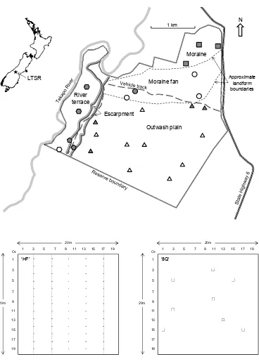
Figure 1. Location and plan of Lake Tekapo Scientific Reserve (LTSR) showing the main geographic and landform features and boundaries. Positions of twelve original sampling plots (established 2003) are indicated as grey symbols (moraine as squares, moraine fan as circles, outwash plain as triangles, river terrace as hexagons and escarpment as pentagons) and positions of twelve new plots (established in 2011) are shown as unfilled symbols.
1 3
11 13 15 17 19 5
7 9
20m Or.
‘HF’ ‘8Q’
20m
20m Or.
20m 1 3 5 7 9 11 13 15 17 19
1 3
11 13 15 17 19 5
7 9
1 3 5 7 9 11 13 15 17 19 Figure 2. Layout of discrete subsampling units within 20 × 20 m vegetation plots for the HF and 8Q sampling methods (left and right, respectively). For each quadrat in the 8Q method, centre peg coordinates are shown in metres from the origin peg (labelled ‘Or.’). The HF and 8Q methods sampled ground areas of 0.65 and 2.0 m2 respectively. A third (‘Recce’) method sampled the entire plot (ground area 400 m2).
3. A modified Recce method (adapted from Hurst & Allen 2007) sampled the whole 400-m2 area of each 20 × 20 m
plot. Percent cover (hereafter ‘Recce cover’), was estimated for each vascular plant species detected to the nearest 1% in each of two height tiers (0–30 cm and 30–100 cm). The cover of a species with <1% cover in any tier was assigned as one of four cover values (1A to 1D) corresponding to 0.25%, 0.625%, 0.1% and 0.0025% cover respectively (which are equivalent to continuous areas of 1 × 1, 0.5 × 0.5, 0.2 × 0.2 and 0.1 × 0.1 m).
Plant origin and life-form groups
Each vascular plant species recorded was assigned to either the exotic or indigenous ‘origin group’ and to one of 13 ‘life-form groups’. Species of dicot composite herb (i.e. eudicot herbs in the family Asteraceae) were split among three groups:
‘hawkweed’ (comprising two exotic mat-forming Pilosella
species), ‘cushion’ (indigenous Raoulia species), and ‘other’. Grasses were also represented by three groups: ‘dwarf grass’ (the xerophytic indigenous Poa maniototo, P. lindsayi and
Agrostis mucosa), ‘tussock’ (indigenous Festuca novae-zelandiae and Poa colensoi), or ‘sward grass’ (both indigenous and exotic). All subshrubs were indigenous and were divided into those with ‘mat’ (Carmichaelia and Coprosma petriei) or ‘erect’ habit (all other species). Remaining groups were ‘dicot non-composite herb’, ‘shrub’ (tall woody species including wilding trees), and three wholly indigenous groups (‘orchid’, ‘rush’ and ‘sedge’). We included a single record of the fern
Pyrrosia elaeagnifolia within the ‘dicot non-composite herb’ group, and of the monocot herb Iphigenia novae-zelandiae
Analyses
We used the software R ver. 3.1.0 (R Core Team 2013) and associated libraries of functions for analyses. Accumulation functions in the ‘vegan’ library (Oksanen et al. 2013) were used for rarefaction, and functions in the ‘Matching’ library (Sekhon 2011) for Kolmogorov–Smirnov tests. Mixed-effects models were fitted with the lmer and glmer functions in the ‘lme4’ library (Bates et al. 2014), and fitted effects were averaged over other model terms with functions in the ‘effects’ library (Fox 2003). All models were checked for conformity with relevant statistical assumptions.
Did plant groups have different abundance and spatial distributions?
Abundance distributions of indigenous and exotic species were represented by empirical cumulative distribution functions (ecdf) of log-transformed Recce cover in each plot. Indigenous and exotic species’ first- and third-quartile ecdf values were compared using paired t-tests, and ecdfs across all plots were compared using a bootstrapped two-sample Kolmogorov–Smirnov test.
We calculated an index of spatial dispersion (or conversely, clustering) as the proportion of ‘8Q’ quadrats (out of eight) in which a species was observed in each plot. Spatial dispersion was fitted as a binomial variable in mixed-effects models with abundance, origin or life-form group, the abundance (i.e. Recce cover) × origin or life-form group interaction, and landform as fixed effects, and species as a random effect. Abundance was represented by cover measured by the Recce method because we required an abundance estimate for each species detection. The life-form-group fixed effect contrasted the other 12 groups with sward grasses, which showed median dispersal overall. Less-dispersed (i.e. more-clustered) origin and life-form groups were expected to occupy fewer 8Q quadrats at any given abundance, indicated by significant negative coefficients for fixed effects in the models.
Did abundance and spatial distributions influence detection?
Simulation was used to test whether different detectability in exotic and indigenous species was explained by differences in their abundance and their spatial distributions (the latter represented by life-form groups). We assessed detection success in the 8Q and HF methods against the standard of the Recce method (which recorded all species that were also recorded by the 8Q or HF methods in any plot, but may have failed to detect certain other cryptic or ephemeral species that were in fact present). We generated three binary conditional detection variables for each species observation:
• ‘Recce alone’ detection was 1 if a species was detected in a plot by the Recce method alone and by neither the 8Q nor the HF method, and 0 if the species was detected by the Recce method and either the 8Q or the HF method. • ‘8Q’ was set to 1 if the species was detected by the 8Q
method as well as the Recce method, and 0 otherwise. • ‘HF’ was set to 1 if the species was detected by the HF
method as well as the Recce method, and 0 otherwise.
We fitted two logistic mixed-effects models of each detection variable. In ‘origin’ models the fixed effect was origin group, and in ‘abundance/life-form’ models fixed effects were the natural log of Recce cover and life-form group. Landform was a covariate and species was a random effect in all models, so that comparisons of detection by various methods were made
within, rather than across species. Model fits were assessed by regressing average per-plot fitted detection probabilities on average observed detection, variance explained was determined using the method of Nakagawa and Schielzeth (2013), and 95% highest posterior density intervals (HPDIs) were calculated for coefficients of each model term.
The three conditional detection probabilities for each species × plot observation were predicted in 1000 draws from the posterior distributions of the fixed- and random-effect coefficients from the ‘abundance/life-form’ models. The median detection probability for indigenous species was subtracted from that for exotic species, and we determined whether 95% confidence of differences between medians excluded zero (indicating significant difference at P < 0.05).
Did method and sample size affect estimates of diversity and indigenous dominance?
We compared species richness and indigenous dominance estimates from multiple plots using rarefaction (an interpolation method that resamples sites without replacement) and Kolmogorov–Smirnov tests. First, we calculated and plotted average cumulative numbers of indigenous and exotic species observed (‘Sobs’) and the average observed indigenous
dominance of composition (% species indigenous, hereafter simply ‘indigenous dominance’) in 1000 random draws of samples of n plots (where n = 3, 4 … 24). The resulting Sobs
and indigenous dominance rarefaction curves were compared between method-pairs using bootstrapped two-sample Kolmogorov–Smirnov tests; this non-parametric test asks whether two samples come from the same distribution, and is sensitive to differences in mean as well as differences in the variance of a distribution (Wang et al. 2003).
We fitted generalised mixed-effects models to compare plot-scale estimates, namely numbers of (1) indigenous, and (2) exotic species recorded per plot (‘species densities’; Gotelli & Colwell 2001), and (3) plot-scale indigenous dominance. In each model, the fixed effect contrasted estimates from the 8Q and HF methods with those from the Recce method, landform was included as a covariate, and plot was an observation-level random effect (which also accounted for over-dispersion; Browne et al. 2005). Species densities were modelled assuming Poisson errors (with a log-link function). Plot-scale indigenous dominance was modelled assuming binomial errors (with a logit-link function) with number of indigenous species as the number of successes and number of exotic species as the number of failures in each ‘trial’ (i.e. plot). As confidence intervals for fixed effects we calculated 95% HPDIs based on 1000 draws from the posterior distribution using functions in the ‘arm’ and ‘coda’ R libraries (Plummer et al. 2006; Gelman & Su 2014).
Results
Indigenous and exotic plant groups had different abundance and spatial distributions
Ln Recce cover
Cumulative probab
ility
-6 -4 -2 0 2 4
0.0 0.2 0.4 0.6 0.8 1.0
Cumulative probab
ility
Cumulative
probab
ility quartile
-6 -4 -2 0 2 4 -6-6 -4-4 -2-2 00 22 44
Third quartile t = −6.083 P < 0.001
Exotic Indigenous
(b) Exotic
(a) Indigenous (c)
Mean t = −6.090 P < 0.001
First quartile t = −2.283 P = 0.031 0.0
0.2 0.4 0.6 0.8
1.0 Quartiles
Figure 3. Abundance distributions of indigenous and exotic plant species in 24 vegetation plots in Lake Tekapo Scientific Reserve. Cumulative probabilities of species occurring at or below a given log-cover abundance (Ln Recce cover) are shown for (a) indigenous and (b) exotic species, with the stepped lines representing the empirical cumulative distribution functions (ecdfs) for species in each plot. In (c), boxplots compare the log-cover abundance values for indigenous and exotic species at the first, second (mean) and third cumulative probability quartiles (which we compared using paired t-tests). In (c) the central boxes show the interquartile range and medians, whiskers (error bars) indicate 10th and 90th percentiles, and open circles show values beyond that range. Vertical grey lines at zero represent 1% cover estimated by the Recce method.
a longer ‘tail’ of low-abundance indigenous species as we had expected, but an even longer ‘leader’ of high-abundance exotic species.
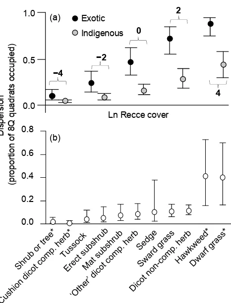
Indigenous species were less spatially dispersed (i.e. more clustered) than exotic species overall; occupying significantly lower percentages of 8Q quadrats at all levels of abundance (origin coefficient −1.50 [−2.28 to −0.74]; Fig. 4a). Differences were greater between indigenous and exotic species that were more abundant (origin × cover interaction coefficient −0.18 [−0.12 to −0.07]), seen as greater disparities in dispersion at the right of Fig. 4a.
Most indigenous species were represented in more clustered life-form groups (Fig. 4b). Tall shrubs (both indigenous and exotic) and indigenous cushion-forming dicot composite herbs were the least dispersed (most clustered) life-form groups, and 95% HPDI indicated that both were significantly less dispersed than our reference sward-grasses group. Low levels of dispersion were also seen in the wholly indigenous ‘tussock’, ‘erect subshrub, ‘mat subshrub, ‘other dicot composite herb, and ‘sedge’ groups, and also in the mixed ‘sward grass’ and ‘dicot non-composite herb’ groups (Fig. 4b). Exotic ‘hawkweed’ and indigenous ‘dwarf grass’ groups were both significantly more dispersed than the reference ‘sward grass’ group.
Abundance and spatial distributions influenced detection
Indigenous species had higher ‘Recce alone’ and lower ‘8Q’ and ‘HF’ conditional detection probabilities than exotic species in our plots (Table 1a–c). Our ‘abundance/life form’ models indicate that abundance and life-form group both significantly affected conditional probabilities of detection (Table 1d–f) and together explained more of the variance in detection than ‘origin’ alone (indicated by higher overall and plot R2 in
Table 1). Simulations from posterior distributions showed that abundance and life-form group together predicted the lower detection probabilities we observed for indigenous species than exotic species (95% confidence intervals in our three ‘difference between medians’ statistics excluded zero; Fig. 5a).
(a)
Ln Recce cover
−4
−2
0
2
4
0.0 0.5
1.0 Exotic Indigenous
Dispersio
n
(p
ro
por
tion o
f 8
Q
q
uadr
ats
o
cc
up
ied)
0.0 0.2 0.4 0.6 0.8
(b)
-6 -4 -2 0 2 4 0.0
0.2 0.4 0.6 0.8 1.0
P
re
di
ct
ed
p
ro
ba
bi
lit
y o
f d
et
ec
tio
n
Ln Recce cover
1D 1C 1B 1A 1% 2% 5% 10% 30%
D
iff
er
en
ce
in
m
ed
ia
n
pro
ba
bi
lit
y
of
d
et
ec
tio
n
(indigenous
species
−
exotic species) 0.0 0.2
HF Recce alone
95% CI [0.08 to 0.26]
95% CI
[–0.39 to –0.14] [–0.34 to –0.13]95% CI
8Q −0.2
−0.4
(a) (b) HF
8Q
Recce alone
Figure 5. Three conditional probabilities of species’ detection (‘Recce alone’, ‘8Q’ and ‘HF’) within 24 vegetation plots in Lake Tekapo Scientific Reserve, predicted from 1000 posterior simulations of coefficients in logistic mixed-effects models. In (a), boxplots show differences in median detection probabilities for indigenous and exotic species in models with species abundance and life-form group fixed effects. Central boxes show the interquartile ranges and medians, whiskers (error bars) indicate 10th and 90th percentiles and open circles show values beyond that range. In (b), labelled bold lines show averages and narrower lines show 95% HPDI of detection probabilities predicted by the model’s abundance coefficient. Vertical grey gridlines indicate untransformed cover levels, including the four values 1A to 1D (corresponding to 0.25%, 0. 625%, 0.1% and 0.0025%, respectively) and the grey background distinguishes species observations with Recce cover <1%.
Table 1. Model-fit statistics and coefficients [and 95% HPDI limits] of fixed effects from logistic mixed-effects models of three (‘Recce alone’, ‘8Q’ and ‘HF’) conditional probabilities of species’ detection in 24 vegetation plots in Lake Tekapo Scientific Reserve. Coefficients are shown on the logit scale of the link function, and statistically significant effects and contrasts are shown in bold. Italic row labels indicate wholly indigenous life-form groups, and the asterisk indicates the single wholly-exotic group (i.e. hawkweeds). N-S R2 is the variance explained by the model calculated according to the method of Nakagawa & Schielzeth (2013), and Plot R2 is the variance explained by a regression of mean detection probability in a plot predicted by the model on the observed data, calculated across all species (and then for exotic and indigenous species separately).
__________________________________________________________________________________________________________________________________________________________________
Recce alone 8Q HF
Conditional probability modelled (1 if the species was detected only by the Recce methods, (1 if the species was detected by both the 8Q and Recce (1 if the species was detected by both the HF and Recce and 0 otherwise) methods and 0 otherwise) methods and 0 otherwise) __________________________________________________________________________________________________________________________________________________________________ ‘Origin’ models: detection ~ origin (indigenous vs exotic) + landform
(a) (b) (c)
Model fit statistics N-S R2 0.21 N-S R2 0.41 N-S R2 0.51
Plot R2 0.32 (0.14, 0.23) Plot R2 0.10 (0.13, 0.10) Plot R2 0.41 (0.19, 0.36)
Origin group coefficient
Indigenous species 0.91 [0.02 to 1.72] −1.01 [−1.89 to −0.22] −1.06 [−2.08 to −0.10] __________________________________________________________________________________________________________________________________________________________________ ‘Abundance/life-form’ models: detection ~ abundance and life-form group (others vs sward grasses) + landform
(d) (e) (f)
Model fit statistics N-S R2 0.56 N-S R2 0.53 N-S R2 0.62
Plot R2 0.48 (0.42, 0.31) Plot R2 0.32 (0.34, 0.38) Plot R2 0.52 (0.75, 0.36)
Abundance coefficient
Ln Recce cover −0.56 [−0.71, −0.43] 0.49 [0.37, 0.59] 0.64 [0.50, 0.77]
Life-form group coefficients
Sward grass <reference group>
Dicot composite herb (erect) 0.56 [−0.54, 1.67] −0.39 [−1.43, 0.55] −0.42 [−1.62, 0.71] Dicot composite herb (cushion) 1.83 [0.78, 2.97] −3.04 [−4.55, −1.71] −1.27 [−2.58, 0.13] Dicot non–composite herb −0.19 [−0.95, 0.60] 0.33 [−0.29, 1.09] 0.23 [−0.62, 1.16]
Dwarf grass −1.51 [−3.50, 0.45] 1.62 [0.21, 3.23] 0.97 [−0.74, 2.80]
Hawkweed* −0.45 [−2.56, 1.24] 1.02 [−0.63, 2.59] 0.11 [−1.81, 2.42]
Mat subshrub 0.47 [−0.92, 1.73] −0.36 [−1.43, 0.78] −1.12 [−2.57, 0.38]
Orchid 0.96 [−0.27, 2.24] −0.07 [−1.34, 1.09] −3.04 [−5.70, −0.83]
Rush 0.27 [−1.70, 2.11] 0.01 [−1.83, 2.03] −1.14 [−3.82, 1.68]
Sedge 0.11 [−1.67, 1.89] 0.10 [−1.55, 1.61] −0.64 [−2.76, 1.52]
Erect shrub 2.45 [1.04, 3.93] −2.08 [−3.63, −0.46] −1.87 [−3.65, −0.23]
Erect subshrub 1.24 [−0.10, 2.56] −0.48 [−1.61, 0.75] −2.22 [−3.80, −0.52]
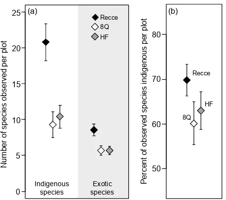
Figure 7. Plot-scale averages and 95% confidence intervals from three sampling methods used to measure 24 vegetation plots in Lake Tekapo Scientific Reserve, showing (a) numbers of indigenous and exotic species observed per plot and (b) percentages of observed species that were indigenous (indigenous dominance of composition).
Less-abundant species were significantly more likely to be detected by the Recce method alone and by neither the 8Q nor the HF subsampling method, as shown by the reverse-s curve of ‘Recce alone’ conditional detection probability on abundance (Fig. 5b) and a negative abundance coefficient in our model (Table 1d). Conversely, rising detection-probability curves (Fig. 5b) and positive abundance coefficients (Table 1e, f) show that the 8Q and HF subsampling methods were more likely to detect more-abundant species, and to miss less abundant species.
Species in the most spatially clustered life-form groups (indicated by lowest dispersion in Fig. 4b) were especially poorly detected by subsampling methods. After accounting for cover-abundance, species in the tall shrub and cushion-forming composite herb (i.e. Raoulia species) life-form groups were most likely to be detected by the Recce method alone (i.e. missed by the 8Q and HF methods) and least likely to be detected by the 8Q method (Table 1d,e). Species of xerophytic dwarf grass (Poa maniototo, P. lindsayii or Agrostis muscosa) (the indigenous life-form group with high dispersion; Fig. 4b) had the lowest ‘Recce alone’ and the highest ‘8Q’ and ‘HF’
0 20 40 60 80
5 10 15 20
65 70 75 80
8Q
HF Recce
(b)
Number of plots
Pe
rc
ent o
f o
bs
er
ved s
pe
cies
in
di
geno
us (
%
)
(a)
5 10 15 20
Numbe
r of
specie
s obse
rve
d (
Sobs
)
8Q (indigenous)
HF (indigenous) Recce (indigenous)
Recce (exotic)
8Q & HF (exotic)
Figure 6. Sample-based rarefaction curves from three sampling methods (Recce – dotted lines, 8Q – solid lines and HF – dashed lines) used to measure 24 vegetation plots in Lake Tekapo Scientific Reserve, showing (a) numbers of indigenous and exotic species observed (Sobs) and (b) percentages of observed species that were indigenous (indigenous dominance of composition) in relation to numbers of plots sampled.
Numbe
r of specie
s
obse
rve
d
per plot
Perce
nt
of
obse
rve
d specie
s
indige
no
us
per
plot
Indigenous
species speciesExotic
0 5 10 15 20 25
50 60 70 80 (a)
Recce 8Q HF
8Q Recce
HF
(b)
detection probabilities and were more likely to be detected by the 8Q method than sward grass species (Table 1d–f). The less-dispersed erect shrub, orchid, erect subshrub and tussock grass life-form groups had the lowest ‘HF’ detection probabilities and were significantly less likely to be detected by the HF method than sward grasses (Table 1f).
Diversity and dominance estimates varied with method and sample size
Our 8Q and HF subsampling methods recorded significantly fewer indigenous and exotic vascular plant species than the Recce (entire-plot) method. They also discriminated more against indigenous species, yielding lower estimates of indigenous dominance (% of observed species indigenous).
These differences were evident across all sample sizes (Figs 6a, b) and also in plot-average statistics (Figs 7a, b). Rarefied estimates of indigenous species Sobs and indigenous
dominance from the Recce method were significantly higher than those from the 8Q and HF methods (bootstrapped Kolmogorov–Smirnov D[Sobs] 0.8636 and 0.9091, D[indigenous
dominance] 0.8636 and 1.000, respectively, all P < 0.001). Sobs
rarefaction curves for indigenous species from the 8Q and HF methods were not significantly different at P < 0.05
(D[Sobs] 0.2273, P = 0.632) but indigenous dominance curves
were (D[indigenous dominance] 0.4091, P = 0.049). At plot scales, 95% HPDI of method coefficients in models of exotic and indigenous richness and indigenous dominance all excluded zero, indicating significant differences between plot-average statistics from the Recce and subsampling methods (Fig. 7).
all methods approached asymptotes at 24 plots, but those for indigenous species continued to rise (Fig. 6a). This pattern suggests further sampling would have encountered more new indigenous species than new exotic species, so that indigenous dominance (Fig. 6b) would also have risen further.
Discussion
Species detection performance and biases
As we predicted, the different abundance distributions and spatial distributions of indigenous and exotic species significantly influenced their likelihood of detection by different vegetation plot sampling methods and sample sizes in our study. This led not only to different estimates of diversity, but also to different ratios of indigenous to exotic species (and therefore indigenous dominance estimates), from different sampling schemes.
Our HF and 8Q subsampling methods, which sampled small areas (totals 0.65 and 2.0 m2, respectively) of each 400
m2 plot, most regularly failed to detect less abundant species.
This detection bias is consistent with the universal prediction that fewer species will be encountered within smaller areas (Rosenzweig 1995) because fewer individuals are sampled (Gotelli & Colwell 2001). However, an important additional consequence was that the overlooked less abundant species were more often indigenous than exotic at our study site, so the proportion of species in the community that are indigenous was systematically underestimated. Irrespective of their abundance, plant species were also less likely to be detected by the two subsampling methods in our study if they were more clustered in space. Furthermore, because more clustered species and plant life-form groups were predominantly indigenous, subsampling doubly discriminated against detection of indigenous plant species.
Together, these results show that the probability of detecting individual plant species in a sampling scheme is determined by their particular characteristics (both abundance and spatial arrangements) and that these characteristics may differ significantly between community components (in our study, between indigenous and exotic floras and among life-form groups). Our finding that these differences can significantly affect estimates of dominance adds to the existing understanding that diversity estimates require more effort where species abundances are uneven (Colwell & Coddington 2004), and that plant detection probabilities vary in a complex manner with community-specific sizes and arrangements of plant clumps and the shape and size of sampling units and plots (e.g. Roxburgh & Chesson 1998; Huebner 2007).
A further novel finding of our study is that irrespective of method, the sampling of small numbers of plots also discriminated against the detection of indigenous species more than the detection of exotic species. Consequently, the percentage of indigenous species rose as the number of plots sampled increased, regardless of sampling method. This ‘sample-size dependence’ (Gotelli & Colwell 2001) of indigenous dominance of composition resembles sample-size dependence in taxonomic ratios, in which larger samples are known to produce higher ratios of species to genera and species to families (Maillefer 1929 cited in Gotelli & Colwell 2001). Taxonomic ratios (species-to-genera or species-to-families) rise because sampling curves for higher taxonomic levels, such as genera or families, reach asymptotes earlier than those
for species nested within them. In our data, larger samples produced higher ratios of indigenous to exotic species because sampling curves for exotic species were lower, flatter, and appeared to be approaching asymptotes earlier than higher and more-continuously-increasing curves for indigenous species.
Implications for community-scale vegetation assessment
Our results caution against two methodological approaches that have been commonplace in published studies of New Zealand’s mixed indigenous–exotic grasslands. These are first, the measurement of vegetation properties within very small areas (typically quadrats or subplots arranged along transects or within larger plots, which we refer to as ‘subsampling’), and second, the use of plot average statistics, rather than rarefaction, to summarise properties of the plant diversity of the community. Our results suggest vegetation statistics derived from small quadrats or subsamples within plots or along transects will be more misleading in plant communities where a high proportion of the floristic diversity is in species with low average abundance and where plant species have conspicuously clustered and uneven spatial distributions. This is consistent with other findings that reliable diversity estimates depend ‘on the portion of the community in the sample; that is, its representativeness’ (e.g. Baltanas 1992).
It would also be unwise to directly compare measures derived from subsampling among different plant community types with different species’ abundance or spatial distributions. For example, differences in species’ abundance or spatial patterns might explain why the height-frequency method performed more poorly in our study than in higher elevation New Zealand tussock grasslands. Dickinson et al. (1997) found a ‘minimum of 75%, and an average of 89%’ of the plant species present within a 5 × 50 m (250 m2) strip also
occurred within sixty 5 × 5-cm height-frequency sampling points. We recorded a minimum of 42%, and an average of 54%, of the plant species present within a 20 × 20 m (400 m2) Recce plot in 65 larger (10 × 10 cm) sampling points.
Detection differences of this magnitude would profoundly alter comparisons of species density and diversity across different plant communities if not accounted for in analyses.
asymptote indicates adequacy of sampling effort, and only asymptotic dominance estimates can be validly compared among communities.
Four community properties are thought to determine shapes of species-area and sampling curves: the size of the species pool, species densities or packing (number of individuals per unit area), the distribution of commonness and rarity, and patterns of intraspecific spatial aggregation or clustering (Preston 1962; May 1988; He & Legendre 2002; Chase & Knight 2013). Rarefaction showed that at least three of these drove significantly different scaling of exotic and indigenous species richness, and hence sample-size dependence of indigenous dominance at our site: there was a smaller pool of exotic species, and a significantly larger pool of less abundant and more-spatially-clustered indigenous species that required greater sampling effort and coverage to intercept. It seems likely that most other mixed indigenous–exotic plant communities in New Zealand (such as exotic forests, shrublands, and a variety of non-woody vegetation types) have indigenous and exotic floras that differ in the size of their species pools and the abundance and spatial distributions of their constituent species. If so, estimates of indigenous compositional dominance that average, rather than accumulate, species numbers across plots in these communities will also be meaningless at community scales.
Conclusions
Sampling smaller areas, subsampling plots (rather than their entire area), and using fewer plots significantly biased downwards estimates of indigenous species richness and dominance of species composition in our study. This was because rare, sparse, spatially-clustered species (which in our study happened to be mainly indigenous) were more difficult to detect than those that were abundant, ubiquitous and/or spatially well dispersed (which were mainly exotic). We conclude that reasonable assessments of species diversity and compositional dominance in mixed grassland plant communities such as ours require (1) systematic searching of plots of sufficient size to ensure coverage of species with low average abundance and uneven spatial distributions (i.e. here, at least 400 m2), and (2) the enumeration and comparison
of floras using rarefaction, rather than plot-scale averaging. Gotelli and Colwell (2001) noted that rarefaction may have been avoided by ecologists in the past because calculations are computationally challenging, but readily available public domain software, such as EstimateS (Colwell 2013) and the ‘vegan’ library for R (Oksanen et al. 2013), have removed this impediment for well over a decade. More routine use of rarefaction should not only improve reliability, transparency, and comparability in the measurement of common vegetation attributes, but also reveal new dimensions of biodiversity patterns and processes in studies of New Zealand’s ecological communities.
Acknowledgements
This work was undertaken as a partnership between the Landcare Research-led Dryland Intermediate Outcome research programme and the Department of Conservation’s Twizel Area Office and Canterbury Conservancy. We thank both the Ministry of Business, Innovation and Employment
and the Department of Conservation for funding. We thank J. McC. Overton for providing generalised tessellated random sampling placements for the new plots, A. Shanks and E. Hayman for help with plant identifications, and W. Lee, A. Tanentzap, J. Tylianakis, and two anonymous reviewers for helpful comments on the manuscript.
References
Allen RB, Rose AB, Evans GR 1983. Grassland survey manual: a permanent plot manual. FRI Bulletin 43. Christchurch, Forest Research Institute.
Baltanas A 1992. On the use of some methods for the simulation of species richness. Oikos 65: 484–492.
Bates D, Maechler M, Bolker B, Walker S 2014. lme4: Linear mixed-effects models using Eigen and S4. R package version 1.1-6. http://CRAN.R-project.org/package=lme4 (accessed 26 September 2014).
Browne WJ, Subramanian SV, Jones K, Goldstein H 2005. Variance partitioning in multilevel logistic models that exhibit overdispersion. Journal of the Royal Statistical Society A 168: 599–613.
Carswell FE, Burrows LE, Hall GMJ, Mason NWH, Allen RB 2012. Carbon and plant diversity gain during 200 years of woody succession in lowland New Zealand. New Zealand Journal of Ecology 36: 191–202.
Chase JM, Knight TM 2013. Scale-dependent effect sizes of ecological drivers on biodiversity: why standardised sampling is not enough. Ecology Letters 16: 17–26. Colwell RK, Coddington JA 1994. Estimating terrestrial
biodiversity through extrapolation. Philosophical Transactions of the Royal Society of London B 345: 101–118.
Colwell, R. K. 2013. EstimateS, Version 9.1.0: Statistical Estimation of Species Richness and Shared Species from Samples (Software and User’s Guide). http://viceroy.eeb. uconn.edu/EstimateS/ (accessed 26 September 2014). Crisp PN, Dickinson KJM, Gibbs GW 1989. Does native
invertebrate diversity reflect native plant diversity? A case study from New Zealand and implications for conservation. Biological Conservation 83: 209–220.
Day NJ, Buckley HL 2013. Twenty-five years of plant community dynamics and invasion in New Zealand tussock grasslands. Austral Ecology 38: 688–699.
Denslow J 1995. Disturbance and diversity in tropical rain forests: the density effect. Ecological Applications 5: 962–968.
Dickinson KJM, Mark AF, Lee WG 1997. Long-term monitoring of non-forest communities for biological conservation. New Zealand Journal of Botany 30: 163–179. Duncan RP, Webster RJ, Jensen CA 2001. Declining plant
species richness in the tussock grasslands of Canterbury and Otago, South Island, New Zealand. New Zealand Journal of Ecology 25(2): 35–47.
Espie PR 1997. Tekapo Scientific Reserve: ecological restoration. Conservation Advisory Science Notes 149. Wellington, Department of Conservation.
Fox J 2003. Effect displays in R for generalised linear models. Journal of Statistical Software 8: 1–27.
procedures and pitfalls in the measurement and comparison of species richness. Ecology Letters 4: 379–391. Green JL, Plotkin JB 2007. A statistical theory for sampling
species abundances. Ecology Letters 10: 1037–1045. He F, Legendre P 2002. Species diversity patterns derived from
species-area models. Ecology 83: 1185–1198.
Huebner CD 2007. Detection and monitoring of invasive exotic plants: a comparison of four sampling methods. Northeastern Naturalist 14: 183–206.
Hurlbert SH 1990. Spatial distribution of the montane unicorn. Oikos 58: 257–271.
Hurst JM, Allen RB 2007. The Recce method for describing New Zealand vegetation – field protocols. Lincoln, Manaaki Whenua - Landcare Research.
Kercher SM, Frieswyk CB, Zedler JB 2003. Effects of sampling teams and estimation methods on the assessment of plant cover. Journal of Vegetation Science 14: 899–906. Lee WG, McGlone M, Wright E 2005. Biodiversity inventory
and monitoring: a review of national and international systems and a proposed framework for future biodiversity monitoring by the Department of Conservation. Lincoln, Manaaki Whenua - Landcare Research.
Leis SA, Engle DM, Leslie JDM, Fehmi JS, Kretzer J 2003.Comparison of vegetation sampling procedures in a disturbed mixed-grass prairie. Proceedings of the Oklahoma Academy of Sciences 83: 7–15.
May RM 1988. How many species are there on earth? Science 241: 1441–1449.
Meurk CD, Norton DA, Lord JM 1989. The effect of grazing and its removal from grassland reserves in Canterbury. In: Norton DA ed. Management of New Zealand’s natural estate. New Zealand Ecological Society Occasional Publication No. 1. Christchurch, New Zealand Ecological Society. Pp. 72–75.
Meurk CD, Walker S, Gibson RS, Espie P 2002. Changes in vegetation states in grazed and ungrazed Mackenzie Basin grasslands, New Zealand, 1990–2000. New Zealand Journal of Ecology 26: 95–104.
Nakagawa S, Schielzeth H 2013. A general and simple method for obtaining R2 from generalized linear mixed-effects models. Methods in Ecology and Evolution. 4: 133–142. Oksanen OJ, Blanchet FG, Kindt R, Legendre P, Minchin PR,
O’Hara RB, Simpson GL, Solymos P, Stevens MHH, Wagner H 2013. Vegan: community ecology package. R package version 2.0-10. http://CRAN.R-project.org/ package=vegan (accessed 8 September 2015).
Plummer M, Best N, Cowles K, Vines K 2006. Coda: convergence diagnosis and output analysis for MCMC. R News 6: 7–11.
Powell KI, Chase JM, Knight TM 2013. Invasive plants have scale-dependent effects on diversity by altering species– area relationships. Science 339: 316–318.
Preston FW 1962. The canonical distribution of commonness and rarity: Part I. Ecology 43: 185–215.
Prosser CW, Skinner KM, Sedivec KK 2003. Comparison of 2 techniques for monitoring vegetation on military lands. Journal of Range Management 56: 446–454.
R Core Team 2013. R: A language and environment for statistical computing. Vienna, Austria, R Foundation for Statistical Computing. http://www.R-project.org/ (accessed 8 September 2015).
McCraw J 1988. The report of the Rabbit and Land Management Task Force to the Right Honorable C.J. Moyle, Minister of Agriculture (Amended version). Mosgiel, The Task Force. 88 p.
Rose AB, Platt KH, Frampton C 1995.Vegetation change over 25 years in a New Zealand short-tussock grassland: effects of sheep grazing and exotic invasion. New Zealand Journal of Ecology 19: 163–174.
Rosenzweig ML 1995. Patterns in space: species area curves. In: Rosenweig ML ed. Species diversity in space and time. Cambridge, Cambridge University Press. Pp. 8–25. Roxburgh SH, Chesson P 1998. A new method for detecting
species associations with spatially autocorrelated data. Ecology 79: 2180–2192.
Scott DM 1965. A height frequency method for sampling tussock and shrub vegetation. New Zealand Journal of Botany 3: 235–260.
Sekhon JS 2011. Multivariate and propensity score matching software with automated balance optimization. Journal of Statistical Software 42(7): 1–52.
Stevens DL, Olsen AR 2004. Spatially balanced sampling of natural resources. Journal of the American Statistical Association 99: 262–278.
Stohlgren TJ, Bull KA, Otsuki Y 1998. Comparison of rangeland vegetation sampling techniques in the central grasslands. Journal of Range Management 51: 164–172. Tomasetto F, Duncan RP, Hulme PE 2013. Environmental
gradients shift the direction of the relationship between native and alien plant species richness. Diversity and Distributions 19: 49–59.
Treskonova M 1991. Changes in the structure of tall tussock grasslands and infestation by species of Hieracium in the Mackenzie country, New Zealand. New Zealand Journal of Ecology 15: 65–78.
Walker S 2000. Post-pastoral changes in composition and guilds in a semiarid conservation area, Central Otago, New Zealand. New Zealand Journal of Ecology 24: 123–138.
Walker S, Wilson JB, Lee WG 2003. Recovery of short tussock and woody species guilds in ungrazed Festuca novae-zelandiae short tussock grassland with fertiliser or irrigation. New Zealand Journal of Ecology 27: 179–190. Wang J, Tsang WW, Marsaglia G 2003. Evaluating
Kolmogorov’s distribution. Journal of Statistical Software 8(18).
Weeks ES, Walker S, Dymond JR, Shepherd JD, Clarkson BD 2013. Patterns of past and recent conversion of indigenous grasslands in the South Island, New Zealand. New Zealand Journal of Ecology 38: 230–241.
Wiser SK, Rose AB 1997.Two permanent plot methods for monitoring changes in grasslands: a field manual. Lincoln, Manaaki Whenua - Landcare Research. https:// nvs.landcareresearch.co.nz/Content/Grassland_manual. pdf (accessed 8 September 2015).
Editorial board member: Jason Tylianakis