On the MAC for Power-Line Communications: Modeling Assumptions and Performance Tradeoffs

On the MAC for Power-Line Communications:

Modeling Assumptions and Performance Tradeoffs

Christina Vlachou

, Albert Banchs

, Julien Herzen

, Patrick Thiran

∗_{EPFL, Switzerland} †_{Institute IMDEA Networks and University Carlos III of Madrid, Spain} ∗ _{[email protected]} † _{[email protected]}

Abstract—Power-line communications are becoming a key component in home networking. The dominant MAC protocol for high data-rate power-line communications, IEEE 1901, employs a CSMA/CA mechanism similar to the backoff process of 802.11. Existing performance evaluation studies of this protocol assume that the backoff processes of the stations are independent (the so-calleddecoupling assumption). However, in contrast to 802.11, 1901 stations can change their state after sensing the medium busy, which introduces strong coupling between the stations and, as a result, makes existing analyses inaccurate.

In this paper, we propose a new performance model for 1901, which does not rely on the decoupling assumption. We prove that our model admits a unique solution. We confirm the accuracy of our model using both testbed experiments and simulations, and we show that it surpasses current models based on the decoupling assumption. Furthermore, we study the tradeoff between delay and throughput existing with 1901. We show that this protocol can be configured to accommodate different throughput and jitter requirements, and we give systematic guidelines for its configuration.

I. INTRODUCTION

Power-line communications (PLC) are increasingly impor-tant in home networking. HomePlug AV, the most popular specification for PLC, is employed by over 120 million devices worldwide [1], and the new HomePlug AV2 devices offer data rates up to 1 Gbps [2]. Moreover, PLC plays a powerful role in hybrid networks comprising wireless, Ethernet, and other technologies [3], as it contributes to increasing the bandwidth of such networks with an independent, widely accessible medium. Yet, despite the wide adoption of HomePlug specifications in home networks, little attention has been paid to providing an ac-curate analysis and an evaluation of the HomePlug MAC layer. The vast majority of HomePlug devices employ a multiple-access protocol based on CSMA/CA that is specified by the IEEE 1901 standard1 _{[4]. This CSMA/CA mechanism} resembles the CSMA/CA mechanism employed by IEEE 802.11, but with important differences in terms of complexity, performance and fairness. The main difference stems from the introduction of a so-calleddeferral counter that triggers a redraw of the backoff counter when a stationsenses the medium busy. This additional counter significantly increases the state-space required to describe the backoff procedure. Moreover, as we explain in more details later, the use of the deferral counter introduces some level of coupling between the stations, which

1_{This CSMA/CA mechanism is the same for all HomePlug specifications,}

including 1.0, AV, AV2 and GreenPhy.

penalizes the accuracy of models based on the decoupling assumption. This assumption was originally proposed in the 802.11 analysis of [5] and has been used in all the works that have analyzed the 1901 CSMA/CA procedure so far (i.e., [6], [7], [8]). In this paper, we show that this decoupling assumption leads to inaccurate results, and the modeling accuracy can be substantially improved by avoiding it.

The decoupling assumption relies on the approximation that the backoff processes of the stations are independent and that, as a consequence, stations experience the same time-invariant collision probability, independently of their own state and of the state of the other stations [5]. In addition, to analyze 1901, it has been assumed that a station senses the medium busy with the same time-invariant probability (equal to the collision probability), during any time slot [6], [7]. In this paper, we show that the deferral counter introduces some coupling among the stations: After a station gains access to the medium, it can retain it for many consecutive transmissions before any other station can transmit. As a result, the collision and busy probabilities are not time-invariant for 1901 networks, which makes the decoupling assumption questionable.

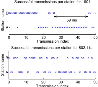
Figures 1 and 2 provide some evidence on the coupling phenomenon described above, for a HomePlug AV testbed with two stations. While Station A transmits during several consecutive slots, StationBis likely to remain in a state where it has a larger probability of colliding or sensing the medium busy. B is then even less likely to attempt a transmission while in this state, and it might have to wait several tens of milliseconds before the situation reverts. Thus, the collision probabilities observed by the stations are clearly time-varying, which invalidates the decoupling assumption. Note that a consequence of this coupling is short-term unfairness, which in turn translates into high delay variance (i.e., high jitter).

0 10 20 30 40 50 A

B

Successful transmissions per station for 1901

Transmission index

Station name

0 10 20 30 40 50

A B

Successful transmissions per station for 802.11a

Transmission index

Station name

59 ms

Fig. 1. Testbed trace of 50 successful transmissions by two saturated stations with 1901 and 802.11a. The experimental settings and the details on our testbed are given in Section V-A. 1901 exhibits short-term unfairness: a station holding the channel is likely to keep holding it for many consecutive transmissions (during several tens of ms, for example 59 ms as shown above), which causes high jitter. 802.11 is fairer, which makes the decoupling assumption viable in this case. This experiment took place under ideal channel conditions. In realistic channels, where frames are retransmitted due to errors, the jitter might even be higher.

0 5 10 15 20

−0.2 0 0.2 0.4 0.6 0.8

Lag

Sample autocorrelation

Sample autocorrelation of X

i

1901

0 5 10 15 20

−0.4 −0.2 0 0.2 0.4 0.6 0.8

Lag

Sample autocorrelation

Sample autocorrelation of X i 802.11a

Fig. 2. We study a testbed trace of5·104 _{successful transmissions for both}

1901 and 802.11a when two saturated stationsAandBcontend for the medium. LetXibe the variable that indicates which station transmits successfully at

thei-th transmission. We takeXi := 1ifAtransmits andXi:= 2 ifB

transmits. We show the autocorrelation function of Xi,1 ≤i≤5·104.

Observe that it is positive for 1901 at lags smaller than15. Hence, ifXi= 1

for somei,it is likely thatXi+1= 1.For 802.11a, we have in contrast a

negative value of autocorrelation at lag 1 and a positive one at lag 2, which means that ifXi= 1for somei,it is likely thatXi+1= 2andXi+2= 1. MAC performance model on a real PLC testbed. We have employed a similar testbed setup to study and validate the short-term unfairness (but not a complete model) of the 1901 MAC in [9]. In addition, we investigate the accuracy of our model and that of previous works that rely on the decoupling assumption, showing that, to the best of our knowledge, ours is the first model for 1901 reaching this level of accuracy. Finally, we study in detail the tradeoff between throughput and delay variance (or equivalently, short-term fairness), caused by the deferral counter in 1901. We observe that this tradeoff can be accurately controlled in 1901, and propose a systematic method to configure a 1901 network to obtain the best delay performance under arbitrary throughput constraints.

The remainder of the paper is organized as follows. We present the 1901 backoff process in Section II. We then review the related work on MAC layer in Section III. We present our model for 1901 in Section IV. We evaluate the performance of our model and discuss the decoupling assumption in Section V. We study the tradeoff between throughput and fairness in Section VI. Finally, we give concluding remarks in Section VII.

II. BACKGROUND

In this section, we present the CSMA/CA protocol of 1901 [4], and highlight the mechanism that causes the strong coupling between the stations. This mechanism is the main difference between 1901 and 802.11. In CSMA/CA protocols, such as 802.11, stations wait for a random number of time slots (determined by thebackoff counter) before transmitting, in the attempt to avoid that some other station transmits at the same slot, which causes a collision. Nevertheless, a collision can still occur and when it does, the stations involved increase the range in which they select their backoff counter (called the contention window CW) to further reduce the collision probability. Clearly, there exists a tradeoff: if CW is large, the collision probability is small, but under low-load conditions stations waste many slots on average before transmitting, which decreases throughput. As we explain later, to tackle this backoff inefficiency, 1901 aims at reducingCW. To counterbalance the resulting large collision probability, 1901 introduces an additional mechanism that increases CW before a collision occurs: when a station senses a considerable number of transmissions in the channel, it increases CW. To count the number of times a station has to sense the medium busy before increasingCW,a new counter is introduced, called the deferral counter.

We now describe the technical details of the 1901 CSMA/CA procedure. It includes three counters: the backoff counter (BC), the deferral counter (DC) and the backoff procedure counter (BP C). Upon the arrival of a new packet, a transmitting station enters backoff stage0. It then draws the backoff counter BC uniformly at random in{0, . . . , CW0−1}, whereCW0denotes the contention window used at backoff stage 0. Similarly to 802.11,BC is decreased by 1at each time slot if the station senses the medium to be idle (i.e., below the carrier-sensing threshold), and it is frozen when the medium is sensed busy. In the case the medium is sensed busy,BCis also decreased by1

once the medium is sensed idle again. WhenBCreaches0, the station attempts to transmit the packet. Also similarly to 802.11, the station jumps to the next backoff stage if the transmission fails. In this case, the station increments the BP C counter and enters the next backoff stage. The station then drawsBC uniformly at random in {0, . . . , CWi−1}, where CWi is

the contention window used for backoff stagei, and repeats the process. For 802.11, the contention window is doubled between the successive backoff stages, i.e.,CWi = 2iCW0.

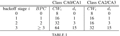
For 1901,CWi depends on the value of theBP C counter and

the priority of the packet: There are four backoff stages that are mapped to the BP C counter, as given in Table I. Also, there are four different priority classes (CA0 to CA3) that correspond to different values for theCWi’s.

The main difference between 1901 and 802.11 is that a 1901 station might enter the next backoff stage even if it did not attempt a transmission. This is regulated by the deferral counter DC, which works as follows. When the station enters backoff stage i,DC is set at an an initialDC valuedi, wheredi is

time

StationA StationB

CWi DC BC CWi DC BC

backoff

stagei backoffstagei

i= 0

i= 1

i= 0

i= 1

i= 0

8 0 3 8 0 5

.

. .. .. .. .. ..

8 0 0 8 0 2

Transmission

8 0 7 16 1 11

.

. .. .. .. .. ..

8 0 0 16 1 4

Transmission

8 0 5 16 0 3

.

. .. .. .. .. ..

8 0 2 16 0 0

Transmission

16_. 1 6 8 0 2

. .. .. .. .. ..

Fig. 3. An example of the time evolution of the 1901 backoff process with 2 saturated stationsAandB. Initially, both stations start at backoff stage0. StationAwins the channel for two consecutive transmissions. Observe the change inCWiwhen a station senses the medium busy and hasDC= 0.

This figure also exposes the short-term unfairness when there are 2 contending stations; a station that grabs the channel for a successful transmission moves to backoff stage 0, whereas the other station enters a higher backoff stage with largerCW and has lower probability to transmit.

the medium busy, a station decreases DC by 1 (in addition to BC). If the medium is sensed busy and DC = 0, then the station jumps to the next backoff stage (or re-enters the last backoff stage, if it is already at this stage) and re-draws BC, without attempting a transmission. An example of such a backoff process is shown in Figure 3.

Class CA0/CA1 Class CA2/CA3

backoff stagei BP C CWi di CWi di

0 0 8 0 8 0

1 1 16 1 16 1

2 2 32 3 16 3

3 ≥3 64 15 32 15

TABLE I

IEEE 1901VALUES FOR THE CONTENTION WINDOWSCWiAND THE INITIAL VALUESdiOF DEFERRAL COUNTERDC,FOR EACH BACKOFF STAGEiAND EACH PRIORITY CLASS. CA0/CA1PRIORITIES ARE USED FOR

BEST-EFFORT TRAFFIC ANDCA2/CA3FOR DELAY-SENSITIVE TRAFFIC.

The deferral counter was introduced in 1901, so that 1901 can employ small contention window values – which provide good performance for a small number of stations – while avoiding collisions, thus also providing good performance for a large number of stations2_{. In particular, to reduce collisions,} 1901 stations redraw their backoff counter when they sense a number of transmissions before their backoff counter expires; in this way, they can react to a high load in the network without the need of a collision, which is in contrast to 802.11 that only reacts to collisions.

Although the above mechanism achieves its goal, i.e., provid-ing good performance in terms of throughput, it might lead to short-term unfairness: When a station gets hold of the channel and uses a small contention window, it is likely to transmit several frames and thus trigger the deferral counter mechanism of the other stations, which further increase their contention windows and hence reduce even more their probability of

2_{Indeed, it can be seen from Table I that 1901 contention windows are small.}

accessing the channel. Such a coupling effect penalizes the accuracy of existing models that assume that the backoff process of different stations are independent. Furthermore, another consequence of this behavior is that a station either holds the channel, and thus experiences low delays, or has to wait a long time before it can transmit. This causes high jitter (i.e., high delay variance).

III. RELATED WORK

The backoff process of 802.11 can be considered as a version of 1901 where the deferral counterDC never reaches

0 (i.e.,di =∞, for all i). Hence, in the following, we first

review relevant studies on 802.11, both with and without the decoupling assumption, and then we present the existing work on 1901. Finally, we discuss related works on fairness.

A. Analyses of IEEE 802.11

Most work modeling 802.11 performance relies on the decou-pling assumption, initially proposed by Bianchi in [5]. In his paper, Bianchi proposes a model for single contention domains, using a discrete-time Markov chain to model the backoff procedure of 802.11. Under the decoupling assumption, the collision probability experienced by all stations is time-invariant and can be found via a fixed-point equation that depends on the parameters of the protocol. Kumar et al. [10] examine the backoff process of 802.11 using the same assumptions and renewal theory. The authors also extract a fixed-point equation for the collision probability. Although strong, the decoupling assumption has later been examined and found to be a valid assumption for 802.11 (shown analytically and experimentally in [11], [12], respectively).

Sharma et al. [13] study 802.11 without the decoupling assumption. They analyze an m-dimensional chain (mbeing the number of backoff stages) that describes the number of stations at each backoff stage. Drift equations capture the expected change on the number of stations at each backoff stage between two consecutive time slots, and their equilibrium point yields the average number of stations at each backoff stage in steady state. Similarly to [13], we also use drift equations to obtain an accurate model for 1901, without resorting to the decoupling assumption. However, as the 1901 protocol is much more complex than 802.11, so is our analysis; it differs substantially from the one of [13].

B. Analyses of IEEE 1901 under the Decoupling Assumption

To the best of our knowledge, the only works analyzing the backoff mechanism of 1901 rely on the decoupling assumption. First, Chung et al. [6] introduce a model using a discrete-time Markov chain similar to Bianchi’s model for 802.11 [5]. The additional state required to capture the effect of the deferral counter DC significantly increases the complexity of the Markov chain.

Finally, Cano and Malone [8] provide a simplification of the analysis of [6] for computing the delay under unsaturated traffic scenarios and discuss the assumptions used in [6]. Here too, their analysis relies on the decoupling assumption.

C. MAC Layer Short-Term Fairness

Various investigations evaluating short-term fairness of MAC protocols have been conducted. First, Berger-Sabbatel et al. [14] study the 802.11 short-term fairness both analytically and experimentally. They prove that the 802.11 MAC is short-term fair when there are few contending stations. Second, Bredel and Fidler [15] elaborate more on the 802.11 backoff process and investigate fairness both in short-term and long-term.

Finally, we explore the 1901 fairness both analytically and experimentally using simulation and a testbed in [9]. We reveal that, compared to 802.11, 1901 is short-term unfair, particularly when there are 2 stations contending for the medium.

IV. ANALYSIS

In this section, we introduce our model for the 1901 CSMA/CA protocol. Our analysis relies on the following assumptions:

• There areN stations that belong to a single contention

domain.

• All stations are saturated (always have a packet to send).

• There is no packet loss or errors due to the physical layer,

and transmission failures are only due to collisions.

• The stations have an infinite retry limit; that is, they never discard a packet until it is successfully transmitted3_. The 1901 standard introduces four different priority classes (see Section II) and specifies that only the stations belonging to the highest contending priority class run the backoff process4. In our analysis, we follow this property, and we consider a scenario in which all the contending stations use the same set of parameters (corresponding to the highest priority class).

Our model is a dynamical system that describes the expected change in the number of stations at each backoff stage between any two consecutive time slots. In the stationary regime, the expected number of stations at each backoff stage is constant, hence we can compute performance metrics by finding the equilibrium of the dynamical system.

Let us now introduce the variables of our model. Letmbe the number of backoff stages and letni,0≤i≤m−1denote the

number of stations at backoff stagei. Note thatPm_i=0−1ni =N.

Let us further denote withτi the transmission probability at

stagei, i.e.,τiis the probability that a station at backoff stagei

transmits at any given time slot. In addition, for a given station at backoff stage i, we denote with pi the probability that at

least one other station transmits. We also denote withpe the

3_{Contrary to 802.11, the 1901 standard does not specify a retry limit.}

However, there is a timeout on the frame transmission that is vendor specific. For instance, for the HomePlug AV devices tested in Section V, the timeout for CA1 priority frames is 2.5s,which is very large compared to the maximum frame duration (2.5ms[4]). Therefore, the infinite retry limit assumption is not strong.

4_{In practice, the contending priority class is decided during a so-called} priority resolution phase, using a simple system of busy tones.

probability that no station transmits (or equivalently, that the medium is idle). Under the assumption of independence of the transmission attempts in a single contention domain, we have pe=

Qm−1

k=0 (1−τk)nk, and therefore

pi= 1−

pe 1−τi

= 1− 1

1−τi m−1

Y

k=0

(1−τk)nk. (1)

In 1901, a station with DC equal to di can change its

backoff stage either (i) after attempting a transmission or (ii) due to sensing the medium busy di+ 1times.5 To compute

the probabilities of events (i) and (ii), we introducexi_k: it is the probability that a station at backoff stagei jumps to the next backoff stage i+ 1ink or fewer time slots due to (ii). Note that we can compute xi_k directly frompi. Let T be the

random variable describing the number of slots amongk slots during which the medium is sensed busy. Because a station at backoff stageisenses the medium busy with probabilitypi at

each time slot, T follows the binomial distribution Bin(k, pi).

This yields

xi_k=P(T > di) = k X

j=di+1

_k

j

pj_i(1−pi)k−j. (2)

Let us denote with bci the expected number of time slots

spent by a station at backoff stage i. Now, recall that when entering stage i, the stations draw a backoff counter BC uniformly at random in{0, . . . , CWi−1}.Let kdenote the

value ofBC, and di be the value of DC when the station

enters stagei.Depending on k, one of the following happens:

• Ifk > di, then event (i) occurs with probability(1−xik),

in which case the station spends (k+ 1) slots in stage i(the (k+ 1)th slot being used for transmission). This event is illustrated by the two transmissions of station A in Figure 3. Now, (ii) occurs with probabilityxi

k. More

precisely, (ii) occurs at slotj, fordi+ 1≤j ≤k,with

probability(xi_j−xi_j−1)6_{, in which case the station spends} j slots in stage i.

• Ifk≤di, then (ii) cannot happen. Event (i) takes place

with probability 1, which yields that the backoff counter expires and that the station spends(k+ 1)slots in stagei. By grouping all the possible cases described above, it follows that bci is given by

bci= 1

CWi CWi−1

X

k=di+1



(k+ 1)(1−xi_k) + k X

j=di+1

j(xi_j−xi_j−1) 



+(di+ 1)(di+ 2) 2CWi

. (3)

Now, the transmission probability τi can be expressed as

a function ofxi_k andbci,using the renewal-reward theorem,

with the number of backoff slots spent in stage i being the

5_{A major difference between 1901 and 802.11 is that, contrary to 1901, a}

station using 802.11 can only adapt its backoff because of (i), not of (ii).

6_{Observe that(x}i

j−xij−1)is the difference of two complementary CDFs

renewal sequence and the number of transmission attempts (i.e., 0 or 1) being the reward. The expected number of transmission attempts at stagei can be computed similarly tobci. Hence,

by dividing the expected transmission attempts at stage iwith the expected time slots spent at stagei,τi is given by

τi=

PCWi−1

k=di+1 1

CWi(1−x

i k) +

di+1

CWi bci

. (4)

Similarly, we define βi as the probability that, at any given

slot, a station at stageimoves to the next backoff stage because it has sensed the medium busy di+ 1times. It can be easily

seen that βi is given by

βi=

PCWi−1

k=di+1 1

CWi

Pk

j=di+1(x

i

j−xij−1) bci

. (5)

Note thatτi andβi are functions ofpi (through xik andbci).

We next introduce our model. A key feature of our model is that we do not assume that the stations are decoupled, as the collision probability is allowed to depend on the station’s state. To study the system, we use a vector that includes the number of stations at each backoff stage. In particular, let X(t) = (X0(t), X1(t), . . . , Xm−1(t))represent the number of stations at each backoff stage (0,1, . . . , m−1) at time slott. We use the notation n(t) = (n0(t), n1(t), . . . , nm−1(t)) to denote a realization ofX(t)at some time slot t.

To analyze our system, we assume that the backoff counters are geometrically distributed with the same mean of that of the real uniform distribution. With this assumption, a station at backoff stageitransmits at any slottwith a constant probability τi given by (4), independently from the previous slots, and the

vectorX(t)is a Markov chain. Furthermore, we assume that at backoff stage i a station might move to the next backoff stage due to sensing the medium busy with probability βi.

Note thatpi, τi,andβican be computed from (1), (4) and (5),

given the state vectorn(t)(hereafter, to simplify notation we drop the input variable t frompi(t), τi(t), βi(t), andn(t)as the equations are expressed for any slot t).

Let now F(n) = E[X(t+ 1)−X(t)|X(t) = n] be the

expected change in X(t) over one time slot, given that the system is at state n. The function F(·) is called thedrift of the system, and is given by

Fi(n) = (DRIFT)

    

   

Pm−1

k=0 nkτk(1−pk)−n0(τ0+β0), i= 0

ni−1(τi−1pi−1+βi−1)−ni(τi+βi), 0< i < m−1

nm−2(τm−2pm−2+βm−2)−nm−1τm−1(1−pm−1), i=m−1. (DRIFT) is obtained by balancing, for every backoff stage, the average rate of stations that enter and leave this backoff stage. In particular, F0 increases only when some stations transmit successfully. Since such stations could be in any of the other backoff stages and there arenk stations in stagek, this occurs

at ratePm_k=1−1nkτk(1−pk).Similarly,F0decreases when some

stations at stage 0 are either involved in a collision (which

occurs with probabilityn0τ0p0), or do not transmit and sense the medium busyd0+ 1 times (which occurs with probability n0β0). The decrease of the drift in both cases is1, thus the expected decrease is equal to the sum of the two probabilities. Similarly,Fi, 0< i < m−1is computed by observing that

in these backoff stages,Fichanges if and only if some stations

sense the medium busy, or transmit. Finally,Fm−1 increases after some stations at stagem−2 experience a collision or sense the medium busydm−2+ 1times. It decreases only after a successful transmission at stagem−1.

Notation Definition (at backoff stagei,0≤i≤m−1) ni Number of stations

pi Probability that at least one other station transmits at any slot

pe Probability that the medium is idle at any slot (same for alli)

xi

k Probability that a station leaves stage i due to sensing the

medium busydi+ 1times (the backoff counter does not expire)

bci Expected number of backoff slots

τi Probability that a station transmits at any slot

βi Probability that a station leaves stage i due to sensing the

medium busydi+ 1times at any slot

Fi Expected change innibetween two consecutive slots ¯

ni Expected number of stations

TABLE II NOTATIONLIST

The evolution of the expected number of stationsn¯(t) := E[X(t)]is described by them-dimensional dynamical system

¯

n(t+ 1) = ¯n(t) +F(¯n(t)), (6)

where F(¯n(t)) is given by (DRIFT). In order to know the average number of stations at each backoff stage at steady state, we can compute the equilibrium point(s) of this system, which is the stationary regime where the average number of stations at each backoff stage remains constant. This information will later enable us to compute actual throughput figures.

Next, we compute the equilibrium point of (6) by imposing F(¯n(t)) = 0,which yields

¯

ni=

_τ

i−1pi−1+βi−1 τi+βi

¯

ni−1, 1≤i≤m−2,

¯

nm−1=

_τ

m−2pm−2+βm−2 τm−1(1−pm−1)

¯

nm−2.

Let us define

K0:= 1, Ki:=

τi−1pi−1+βi−1 τi+βi

, 1≤i≤m−2, Km−1:=

τm−2pm−2+βm−2 τm−1(1−pm−1)

. (7)

Since Pm_i=0−1n¯i = N, it follows that the equilibrium of

system (6) is given by the following system of equations:

¯

n0=

N

Pm−1

k=0

Qk j=0Kj

,¯ni=

NQi_j=0Kj Pm−1

k=0

Qk j=0Kj

1≤i≤m−1. (EQ)

Recall thatτiandβiare functions ofpi, given by (4) and (5).

Thus, then¯i’s in (EQ) are also functions ofpi,0≤i≤m−1.

following theorem is one of our main results. It states that, for configurations satisfying CWi+1≥2CWi−di−1, 0≤

i < m−1, the system (EQ), (1) admits exactly one solution, hence that the equilibrium point of (6) is unique. Note that, from Table I, these constraints are compliant with the standard, except for the class CA2/CA3 at backoff stagei= 1. We leave the extension of the uniqueness result to this priority class, and the investigation of the stability of (6) for future work.

Theorem 1. Assume that CWi ≥ 6 and di ≤ bCWi/2− 1c, 0 ≤ i ≤ m−1. In addition, assume that CWi+1 ≥

2CWi−di−1, 0≤i < m−1. Then the system of equations formed by (EQ) and (1) has a unique solution.

Proof:Recall that pe=Qm_k=0−1(1−τk)n¯k. For any value

ofpe, τi can be computed from the fixed-point equation that

results from combining (1) (i.e., pi = 1−pe/(1−τi)) with

(4), where (4) is expressed as a function of pi through (2)

(see [16] for more details). Hence, τi can be computed as

a function of pe, and so can pi, βi. Now, n¯i can also be

computed as a function of pe, given (EQ). With this, let Φ(pe) :=Qm_k=0−1(1−τk(pe))n¯k(pe)_{. Then, a solution of (EQ)}

has to satisfy the following equation:

pe= Φ(pe). (8)

We next show that there exists only one value of pe that

satisfies (8). Due to space constraints, we show in [16] that

Φ(pe)has at least one fixed-point. To this end, we show that

Φ(pe)is monotonically decreasing withpe. The derivative of Φ(pe)can be written as

dΦ(pe)

dpe =

m−1

X

j=0

_∂Φ

∂pj

∂pj

∂pe + ∂Φ

∂βj

∂βj

∂pe + ∂Φ

∂τj

∂τj

∂pe

. (9)

We now examine separately each of the partial derivative products of (9) with respect to pj, βj andτj.

First, Lemmas 1 and 2 in Appendix imply respectively that ∂pj/∂τj < 0 and ∂τj/∂pe < 0. Because ∂pj/∂pe = (∂pj/∂τj) · (∂τj/∂pe), we have ∂pj/∂pe < 0. Also, by

Lemma 5 in Appendix,∂Φ/∂pj>0.Thus, the first product

of partial derivatives in (9) is negative for all j. Second, by Lemma 3 in Appendix, ∂Φ/∂βj≥0.Now, Corollary 2 states

that∂βj/∂pj >0and we have shown above that∂pj/∂pe<0.

Hence, we have∂βj/∂pe<0,and the second product of partial

derivatives in (9) is also negative. Third, by Lemma 4 we have ∂Φ/∂τj<0,and by Lemma 2 we have∂τj/∂pe>0. We thus

have shown that all the partial derivative products of (9) are negative, and soΦ(pe)is monotonically decreasing with pe.

Since (9) is strictly negative, there exists a unique value for pe that solves (8). Computing the corresponding value forpi

by (1), we have a solution to (EQ). The uniqueness of the solution then follows from the fact that all relationships between τi, βi, piandpeare bijective, and any solution must satisfy (8),

which (as we have shown) has only one solution.

In Section V, we observe that our model is very accurate for all configurations. We explain how collision probability and throughput are computed in the same section.

V. PERFORMANCEEVALUATION

In this section, we evaluate the 1901 performance under different configurations. First, we validate experimentally our simulator and our model by using a testbed. Second, we evaluate our model and compare it with the models based on the decoupling assumption [6], [7]. These models perform different computations, but are strictly equivalent in terms of predicted throughput. We thus refer to these models as (the unique) “D.A.” model.

A. Experimental Validation

We use simulations to evaluate 1901 performance. We wrote a Matlab simulator, which implements the full CSMA/CA mechanism of 19017. In this subsection, we validate the accuracy of our model and simulator with experimental results from a HomePlug AV test-bed.

We built a test-bed of 7 stations, each comprising a PLC interface8. The stations are ALIX boards running the OpenWrt Linux distribution [18]. Each board is equipped with a Homeplug AV miniPCI card (Intellon INT6300 chip). In our tests,N stations send UDP traffic (at a rate higher than the link capacities) to the same non-transmitting station using iperf. We run tests for1≤N ≤6.At the end of each test we request the number of collided and successfully transmitted frames from each station using theQualcomm Atheros Open Powerline Toolkit[19]. Using this information, we evaluate the collision probability.

We compare the collision probability measured on the testbed with the one obtained with our model. To this end, we use our model to compute the steady-state expected number of nodes

¯

n0, . . . ,n¯m−1at each backoff stage. Once we have the average number of stations at each each backoff stage, the probability pi of collision at backoff stagei is readily given by (1).

Let γ be the average probability that a transmission in the system collides. The probability that a given transmis-sion in the system corresponds to a station at backoff stage i is given by n¯iτi/

Pm−1

k=0 n¯kτk. We thus have γ = Pm−1

i=0 n¯iτipi/ Pm−1

i=0 ¯niτi.

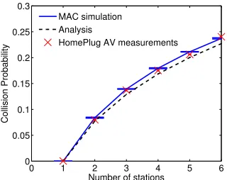
The average collision probabilities obtained from 10 testbed experiments, 10 simulation runs, and our model are shown in Figure 4. We observe an excellent fit between experimental and simulation/analytic results.

Contrary to some existing 802.11 interfaces, the MAC parameters of the HomePlug AV devices cannot be modified, because they are stored in the firmware, and the required offsets of their binary values are not publicly available. Therefore, the results on throughput and fairness have been obtained with our validated simulator.

7_{Our simulator and the guidelines to reproduce all the testbed experiments}

of this work are available in [17].

8_{The stations also have a wireless interface, a miniPCI card Atheros}

0 1 2 3 4 5 6 0

0.05 0.1 0.15 0.2 0.25 0.3

Number of stations

Collision Probability

MAC simulation Analysis

HomePlug AV measurements

Fig. 4. Collision probability obtained by simulation, our drift model of Section IV and experiments with HomePlug AV devices for the default configuration CA1 of 1901 given in Table I.

B. Simulation Parameters and Throughput Computation

Our simulator uses the same time slot duration and timing parameters as specified in the standard (see Table III). The PLC frame transmission has a duration D and is preceded by two priority tone slots (P RS), and a preamble (P). It is followed by a response inter-frame space (RIF S), the ACK, and finally, the contention inter-frame space (CIF S). Thus, a successful transmission has a durationTs:= 2P RS+P+D+RIF S+

ACK +CIF S. In the case of a collision, the stations set the virtual carrier sense (VCS) timer equal to EIF S,where EIF S is the extended inter-frame space used by 1901, and then the channel state is idle. Hence, a collision has a duration Tc:=EIF S.Finally, we assume that all the packets use the

same physical rate.

Parameter Duration (µs)

Slotσ, Priority slotP RS 35.84

CIF S,RIF S 100.00

PreambleP,ACK 110.48

Frame durationD 2050.00

EIF S 2920.64

TABLE III SIMULATION PARAMETERS.

To analytically evaluate throughput, we employ the model of Section IV. After solving the equations for finding the steady-state number of nodes n0, . . . ,¯ ¯nm−1 at each backoff stage, we can compute the throughput of the network as follows. The probability that a slot is idle is pe.The probability of a

successful transmission of a station at stage i is τi(1−pi). Therefore, the probability ps that a slot contains a successful

transmission is given by ps = Pm−1

i=0 n¯iτi(1−pi). Let pc

denote the probability that a slot contains a collision. We have pc= 1−pe−ps.We now have enough information to compute

the normalized throughputS of the network as

S = psD

psTs+pcTc+peσ

, (10)

whereDis the frame duration,Tsis the duration of a successful

transmission, Tc is the duration of a collision, and σ is the

time slot duration.

C. The Decoupling Assumption Does Not Hold for 1901

For 802.11, the decoupling assumption has been shown to be viable in various settings as N → ∞ [11]. In addition,

0 1 2 3 4 5 6

0 0.1 0.2 0.3 0.4 0.5

Backoff stage

Collision Probability

802.11 MAC

N = 2 N = 5 N = 10 N = 10

N = 5

N =2

0 1 2 3

0 0.1 0.2 0.3 0.4

Backoff stage

Collision Probability

1901 MAC

N = 2 N = 5 N = 10 N=10

N = 5

N = 2

0 1 2 3

0 0.05 0.1 0.15 0.2 0.25

1901 MAC

Backoff stage

Collision probability Drift model

Simulation

Fig. 5. Simulations of 1901 (with CA1 parameters) and 802.11 forN = 2,5,10.Points show the collision probabilities at different backoff stages for all stations, and lines represent the solution of the fixed-point equations for the collision probability from the D.A. models [5], [7]. The decoupling assumption is viable for 802.11 even forN= 2,whereas the collision probability depends on the backoff stage for 1901. Our model accurately predicts the collision probability at each backoff stagei(shown at the right forN= 2). it turns out that it also works well for small numbers of stations [5], [12]. For 1901, the coupling induced by the deferral counter makes the collision probabilities state-dependent, which penalizes models based on the decoupling assumption when N is small. To see this, we plot on Figure 5 the collision probabilities experienced by 802.11 and 1901 stations, as a function of the backoff stage (i.e., as a function of the stations’ state). On the same figure, we also show the collision probabilities computed with our model. LetCkbe the sequence

of outcomes of attempted transmissions, i.e.Ck:= 0if thekth

transmission attempt results in a success, andCk := 1 when

the outcome is a collision. The decoupling assumption asserts that the sequence{Ck}consists of independent and identically

distributed (i.i.d.) random variables. In Figure 5, we observe that for 1901,{Ck}cannot be considered as i.i.d., because the

collision probability observed at different backoff stages is not the same. The collision probability depends on the previous transmission attempts (backoff stage changed due to collision) or on other stations activity (backoff stage changed due to sensing the medium busy). In fact, the collision probability for 1901 is an increasing sequence of the backoff stagei, as shown in Figure 5, and proved in Corollary 1 in Appendix.

D. Model Evaluation

CA1 uses larger contention windows, which increases the time spent in backoff and, as a result, the coupling between stations.

0 2 4 6 8 10

0.5 0.55 0.6 0.65 0.7 0.75

Number of stations

Normalized throughput _{D.A. model}

Simulation Drift model

CA1

CA3

Fig. 6. Throughput obtained by simulation, with our model, and the models based on the decoupling assumption (D.A.), for the default configurations of 1901 given in Table I.

We now study the accuracy of the two models in more general settings. To this end, we introduce a factorf, such that at each stagei, the value ofdiis given bydi=fi(d0+ 1)−1. This enables us to define various sequences of values for the di’s, using only f andd0. At each stagei, CWi is given by

CWi= 2iCWmin,and there arembackoff stages (i∈ {0, m− 1}). In Figure 7, we show the throughput for various such values of d0 and f, withCWmin = 8andm= 4. We observe that

the D.A. model achieves good accuracy when thedi’s are large,

because in these configurations, the deferral counter is less likely to expire, which reduces the coupling among stations. Note that the drift model achieves good accuracy when the di’s are small.

0 5 10 15 20 25 30 35

0.35 0.4 0.45 0.5 0.55 0.6 0.65 0.7 0.75 0.8

Number of stations

Normalized throughput

m = 4, CW_min = 8

D.A. model Simulation Drift model

d₀ = 1, f = 2 d₀ = 0, f = 2 d₀ = 0, f = 1

d₀ = 3, f = 2

Fig. 7. Throughput obtained by simulation, with the drift model, and the D.A. model for different configurations. The initial valuesdiof the deferral counter

at each backoff stage are given bydi=fi(d0+ 1)−1.

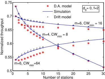
Finally, in Figure 8 we show the throughput for different values for CWmin, with m ∈ {4,6}. In all cases, the drift

model fits very well, contrary to the model based on the decoupling assumption. The accuracy of the D.A. model is penalized more when CWmin is large, because the likelihood

that the deferral counter expires increases.

VI. THROUGHPUT, FAIRNESS ANDCOUPLING In this section we show how the coupling between 1901 stations is related to throughput and jitter (or, equivalently,

0 5 10 15 20 25 30

0.5 0.55 0.6 0.65 0.7 0.75

Number of stations

Normalized throughput

d₀= 0, f=2 D.A. model

Simulation Drift model

m=6, CW_min = 16

m=4, CW min = 8

m=6, CW_min=64

Fig. 8. Throughput obtained by simulation, with the drift model, and the D.A. model for various values ofCWminandm∈ {4,6}.

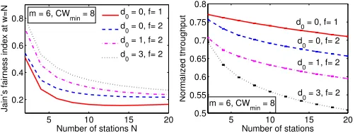
unfairness). Moreover, based on our model, we propose a method to optimize jitter under a given throughput requirement. In the introductory example of Figure 1, we observe a bistability effect with two 1901 stations, where stations are likely to remain for long durations in states with large transmit (resp. backoff) probabilities. We explain that this effect is caused by the deferral counter, which creates a coupling between the stations and penalizes the accuracy of models assuming decoupling. It turns out that this coupling is beneficial for throughput9, and different 1901 configurations determine different tradeoffs between fairness (or jitter) and throughput. We now investigate this effect further in terms of short-term fairness. A MAC protocol is short-short-term fair when the stations get similar transmission opportunities over short time scales. Conversely, an unfair protocol advantages some stations over others, which in practice results in high delay variance (jitter). To measure short-term fairness, we compute Jain’s fairness index [20] over windows of N frame durations. More precisely, if we let xi(w) be the number of frames successfully transmitted by station i during a window ofw frame durations, Jain’s index during window wis defined as J(w) = (PN_i=1xi(w))2/(NPN_i=1xi(w)2). In the following, we take w=N, as this is the smallest value of wsuch that J(w) can be equal to 1 (for a perfectly fair protocol). The reported results are obtained by averaging the values ofJ(N)

over windows moving along the whole packet traces. In Figure 9, we plot throughput and short-term fairness as a function of the initial values of the deferral counter (in terms of d0 and f), for N = 2 and N = 5. Interestingly, it appears that that there is a direct link between throughput, fairness and coupling. When the initial deferral counters are small (corresponding to smalld0 andf), the stations are more likely to react on sensing the medium busy and thus become coupled. Indeed, as confirmed by Figure 7, the configurations employing small deferral counters yield larger throughput but lower accuracy when assuming decoupling. Conversely, these configurations have the worse short-term fairness and thus cause higher jitter.

We study further the throughput/fairness tradeoff on

Fig-9_{Intuitively, this is easy to understand: without proper synchronization,}

{0,1} {0,2} {1,2} {3,2} 0.3

0.4 0.5 0.6 0.7 0.8

Configuration {d₀,f} Throughput Fairness

{0,1} {0,2} {1,2} {3,2} 0.3

0.4 0.5 0.6 0.7 0.8

Configuration {d₀,f} Throughput Fairness

Fig. 9. Throughput and fairness withCWmin= 8andm= 4and various

values ofd0andf, forN= 2(left) andN= 5(right). The initial value of

the deferral counter at backoff stageiis given bydi=fi(d0+ 1)−1.

5 10 15 20

0.2 0.4 0.6 0.8

Number of stations N

Jain’s fairness index at w=N

m = 6, CW

min = 8 d0 = 0, f= 1

d

0 = 0, f= 2

d

0 = 1, f= 2

d

0 = 3, f= 2

5 10 15 20

0.5 0.55 0.6 0.65 0.7 0.75 0.8

Number of stations

Normalized throughput _{m = 6, CW}

min = 8

d₀ = 0, f= 1

d₀ = 0, f= 2

d₀ = 3, f= 2

d₀ = 1, f= 2

Fig. 10. Short-term fairness and throughput obtained by simulation for parameters CWmin = 8, m = 6 and various values of d0 andf. The

deferral counter tunes a tradeoff between throughput and fairness in 1901.

ures 10 and 11. Both figures show the throughput and fairness achieved on networks with a varying number of stations. Figure 10 presents throughput and fairness for various initial deferral counter values (in terms ofd0andf). Figure 11 shows these two metrics for different numbers of backoff stages m.

Again, both figures show a clear tradeoff between throughput and short-term fairness. Furthermore, this tradeoff can be tuned by adapting the parameters that control the number of backoff stages and the initial values of the deferral counters. This possibility is a remarkable feature of 1901, enabled by the deferral counter. We summarize the impact of all parameters on throughput and fairness in Table IV.

A. Finding Efficient Configurations

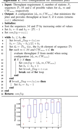
We can use the findings summarized in Table IV, together with our drift model, to find efficient configurations that meet specific QoS criteria. For example, we propose a simple heuristic algorithm that finds an efficient configuration in terms of jitter, given an arbitrary throughput requirement (if such a configuration exists). Our method is detailed in Algorithm 1 and works as follows. It orders (by increasing order of values) the sets of possible values taken byd0andmin two sequences named D and M, respectively. It then performs a binary search on D: for a given d0 in D, it tests all combination of parameters(m, CWmin)(by increasing order ofm). When

such a configuration satisfies the throughput requirement, the algorithm stores it and tries a larger value for d0 (as a largerd0 can potentially yield better jitter). Conversely, if no configuration meeting the throughput requirement is found, the algorithm considers smaller values ford0 (which yield higher throughputs, potentially at the expense of jitter). The algorithm ends when it finds the best configuration that corresponds to the largest possible d0 that satisfies the constraint.

5 10 15 20

0.2 0.3 0.4 0.5

Number of stations N

Jain’s fairness index at w=N

CW

min = 8, d0 = 0, f = 2

m = 4

m = 6 m = 5

5 10 15 20

0.55 0.6 0.65 0.7 0.75

Number of stations

Normalized throughput

CW_min = 8, d₀ = 0, f = 2

m = 5 m = 6

m = 4

Fig. 11. Short-term fairness and throughput obtained by simulation with parametersCWmin= 8, d0= 0, f= 2and various values ofm.

d0 f m CWmin

small T% T% T& T%ifN is small

F& F & F% F→

large T& T& T% T%ifN is large

F% F % F& F→

TABLE IV

SUMMARY OF THE QUALITATIVE EFFECTS OF EACH PARAMETER ON THROUGHPUT(“T”)AND SHORT-TERM FAIRNESS(“F”). Because it employs a binary search, the complexity of this algorithm is O(|C| · |M| · log(|D|)). We evaluate it on the sequences C = (8,16,32,64), M = (4,5,6) and

D= (0,1,2,3)10. First, we run simulations of all the possible configurations in{C × M × D},and we compute short-term fairnessJ(N)and normalized throughput S.LetSmin be the

minimumS achieved by all configurations in{C × M × D}, and similarlySmaxbe the maximum S.To test our algorithm,

we draw 100 throughput requirements uniformly at random in

[Smin, Smax].Then, for each sampleiwith throughputSi, we

run Algorithm 1 that returns the configuration conf igi.Now,

letJibe the short-term fairness of the configurationconf igiat

samplei,and letJmax

i denote the maximum short-term fairness

of all configurations that satisfy the throughput constraintSi.

To evaluate the algorithm, we employ a normalized fairness index that is defined asJi/Jimax.The normalized fairness is

a metric that evaluates the distance between the fairness of the configuration conf igi and the maximum achievable fairness

given the the throughput constraintSi.

The results of the algorithm evaluation are presented in Figure 12. We present the normalized fairness of the configu-rations returned from 100 runs of Algorithm 1. We repeat the procedure described above for2≤N ≤8.We observe that Algorithm 1 always returns a configuration with good fairness given the throughput constraint. Thus, it can be employed to optimize the performance for delay-sensitive traffic that operates with 1901.

VII. CONCLUSION

The IEEE 1901 CSMA/CA protocol has received little attention from the research community so far, although it is adopted by the vast majority of power-line communication devices. In this paper, we focus on the analysis of the performance of this protocol. One of the key results is the

10_{We use the factorf= 2because the contention windows are also doubled}

Algorithm 1: 1901 configuration for minimum jitter

1 Input:Throughput requirementS, number of stationsN, sequencesD,MandC of possible values ford0,mand CWmin, respectively

2 Output: A configuration(d0, m, CWmin)that minimizes the jitter and provides throughput at leastS, if it exists (returns

nullotherwise)

3 Initialize:

4 Sort the sequencesMandDby increasing order of values 5 Seth1←0andh2← |D| −1

6 Setconf ig←null

7 whileh1≤h2 do

8 Setbreak f lag←false

9 h3← d(h2−h1)/2e+h1

10 Setd0 ← Dh3 (i.e., theh3-th element of sequenceD)

11 foreachm∈ MandCWmin∈ C do

12 evaluate throughputSˆfrom model when using

configuration(d0, m, CWmin)

13 ifSˆ≥S then

14 Setconf ig←(d0, m, CWmin)

15 Seth1←h3+ 1

16 Setbreak f lag←true

17 break out offorloop

18 end

19 end

20 ifbreak f lag==falsethen

21 Seth2←h3−1

22 end

23 end

24 Return: conf ig

0.88 0.9 0.92 0.94 0.96 0.98 1

2 3 4 5 6 7 8 N

Normalized fairness

Fig. 12. Normalized fairness of the configurations Algorithm 1 returns when run for 100 throughput requirementsSchosen randomly, for eachN value. finding that the decoupling assumption, which is commonly adopted for the analysis of MAC protocols such as IEEE 802.11 and IEEE 1901, might not hold for 1901. This is due to the coupling that this protocol introduces to the stations contending for the medium. Building on this finding, we have proposed a new model that does not rely on the decoupling assumption and thus substantially improves the accuracy of previous studies, in particular for networks with a small number of stations, the most frequent configuration in practice. Our model reveals that, as a result of the coupling between stations, 1901 suffers from short-term unfairness. To address this issue, we have explored the tradeoff between short-term fairness and throughput that exists in 1901. In this context, we devised a method that computes efficient configurations in terms of fairness/jitter, under arbitrary throughput constraints.

APPENDIX

We provide the sketch of the proof of some necessary lemmas for Theorem 1. The detailed proofs can be found in [16].

Lemma 1. τi is a decreasing function ofpi for anyi.

Proof:The probability τi given by (4) can be recast as

τi= 1

Bi+ 1

(11)

whereBi is the expected number of backoff slots between two

transmission attempts of a station that always stays at backoff stagei.Bi can be computed recursively and is given by

Bi=

di(di+ 1) 2CWi

(12)

+ CWi−1

X

j=di+1

j(1−xi j) +

Pj

k=di+1(k+Bi)(x

i

k−x

i k−1) CWi

.

To prove the lemma, we need to show thatBiis an increasing

function ofpi. To do this, we proceed as follows. (i) First, we

compute the derivative of Bi with respect topi. (ii) Second,

we show that this derivative is positive at pi= 1. (iii) Third,

we further show that if the derivative is negative for some

0 < p∗_i <1, it will also be negative at any value pi > p∗i.

The proof then follows by contradiction: If the derivative was negative at somep∗_i, it would also be negative atpi = 1, which

would contradict our previous result (ii).

(i) After simple manipulations, (12) can be recast as

Bi=

CWi−1

2 +

1

CWi CWi−1

X

j=di+1

Bixij− j−1

X

k=di+1 xi_k

!

. (13)

The derivative ofBi can be computed as

dBi

dpi =

CWi−1

X

k=di+1 ∂Bi

∂xi k

∂xi k

∂pi

. (14)

The partial derivative∂Bi/∂xik can be computed from (13) as

∂Bi

∂xi k

= Bi−(CWi−1−k)

CWi

+∂Bi

∂xi k

CWi−1

X

j=di+1 xi

j

CWi

, (15)

which yields

∂Bi

∂pi =

PCWi−1

k=di+1(Bi−(CWi−1−k))

∂xi k

∂pi CWi−PCW_j=di_i−₊₁1xij

. (16)

To compute∂xi

k/∂pi, we observe thatxik is the

complemen-tary cumulative function of a binomial distribution. By taking its partial derivative, we obtain

∂xi_k ∂pi

= k!

(k−di−1)!di!

pdi

i (1−pi)

k−di−1_{, (17)}

which ends the computation of dBi/dpi.

(ii) Next, we show thatdBi/dpi>0atpi= 1. We have

Bi=

di(di+ 1) 2CWi

+CWi−di−1

CWi

(di+ 1 +Bi). (18)

Solving (18) overBiyieldsBi=CWi−di/2−1atpi= 1.

Substituting in (16), it follows thatdBi/dpi =di/2 + 1>0

(iii) Finally, we show that ifdBi/dpi was negative at some

valuep∗

i, then it would also be negative for any larger value of

pi. Observe that in (16) some terms are negative fork < CWi− 1−Bi. Let us assume that the derivative is negative atp∗i.

Then, at somepi=p∗i +, >0, we haveBi(pi)< Bi(p∗i).

This implies that in (16) some of the terms that were positive withpi=p∗i become negative for pi> p∗i. Furthermore, from

(17) we have that

∂xi_k/∂pi

∂xi k−1/∂pi

= k

k−di−1

(1−pi), (19) which implies that in (16) the relative weight of the negative terms increases and that of the positive terms decreases.

From the above, it follows that if dBi/dpi was negative at

any p∗_i, it would also be negative for all pi > p∗i. Since this

contradicts the above result thatdBi/dpi is positive atpi= 1,

we conclude thatdBi/dpi≥0 forpi∈[0,1].

Corollary 1. τi is a strictly decreasing sequence of i,and pi is a strictly increasing sequence of i if CWi+1 ≥2CWi−

di−1, 0≤i < m−1.

Proof: The minimum value of Bi+1 is Bimin+1 :=

(CWi+1 −1)/2 at pi+1 = 0, and the maximum value of Bi is Bimax := CWi −di/2 −1 at pi = 1. Setting

CWi+1 ≥ 2CWi−di −1, yields Bimin+1 ≥ Bimax, hence

Bi+1> Bi andτi+1< τi. Now, pi is strictly increasing with

i becausepi= 1−pe/(1−τi).

Corollary 2. βi is an increasing function of pi.

Proof:From (4) and (5) we haveβi= 1/bci−τi. (3) can

be recast asbci= (CWi+1)/2−

PCWi−1

k=di+1

Pk j=di+1x

i j/CWi.

By (17) we have dxi_k/dpi >0, hencebci is decreasing with

pi.Using Lemma 1, βi= 1/bci−τi is increasing withpi. Lemma 2. Let us consider the expression ofτi as a function of peresulting from combining (4) with (1). According to this expression, τi is an increasing function ofpe, ifCWi≥6and

di≤ bCWi/2−1c.

Proof:The details on howτican be expressed as a function

ofpe can be found in [16]. Sinceτi= 1/(Bi+ 1), we need

to show that∂Bi/∂pe<0. Note that

∂Bi

∂pe =∂Bi

∂pi

∂pi

∂pe

. (20)

Becausepi= 1−pe/(1−τi) = 1−pe(Bi+ 1)/Bi, we have

∂pi

∂pe

=−Bi+ 1

Bi

+ pe

B2

i

∂Bi

∂pe

. (21)

Combining (20) and (21) yields

∂Bi

∂pe

=−∂Bi

∂pi

Bi+ 1

Bi

1

1− pe

B2

i

∂Bi

∂pi

. (22)

Because of Lemma 1, ∂Bi/∂pi > 0, and therefore

∂Bi/∂pe<0as long as

∂Bi

∂pi

< B 2

i

pe

=Bi(Bi+ 1) 1−pi

. (23)

From (16) we have

∂Bi

∂pi

< Bi CWi−

PCWi−1

k=di+1x

i k

CWi−1

X

k=di+1 ∂xi_k

∂pi

. (24)

First, let us study (24) with di = 0. We have∂xik/∂pi =

k(1−pi)k−1 _andxi

k = 1−(1−pi)k.Thus, (24) yields

∂Bi

∂pi

< Bi

1−pi

PCWi−1

k=0 k(1−pi)

k

PCWi−1

k=0 (1−pi)k

≤ B

2

i 1−pi

. (25)

Define h(pi) := PCWi−1

k=0 k(1−pi)

k_/PCWi−1

k=0 (1−pi)

k_.

The last inequality in (25) holds because first, h is strictly decreasing withpi in [0,1]using Lemma 5.1 in [10], hence

h(pi)≤h(0) = (CWi−1)/2.Second,Bi(pi)≥(CWi−1)/2

using the proof of Lemma 1.

We now move to the casedi6= 0. We show that∂Bi/∂pi<

B2

i, which is sufficient for (23) to hold. From (17) and (2), we

have∂xi

k/∂pi=k(xik−xik−1)/pi. Thus, (24) yields

∂Bi

∂pi

< Bi pi

CWixiCWi−1−

PCWi−1

k=di+1x

i k

CWi−PCW_k=di_i−₊₁1xi_k

≤ Bi

pi

xi_CWi−1.

Letg(pi) =Bipi−xiCWi−1. Now, it is sufficient to show that ∂g/∂pi >0 for pi ∈ (0,1], because g(0) = 0. Let X be a

random variable following the binomial distribution Bin(CWi− 2, pi). Then, observe that

∂g ∂pi

=Bi+

∂Bi

∂pi

pi−(CWi−1)P(X=di). (26)

SinceBi≥(CWi−1)/2, ∂g/∂pi >0 if P(X =di)<1/2.

The maximum of P(X =di) is at pi =di/(CWi−2). We

show that P(Y = di) < 1/2, where Y now is a random

variable following the distribution Bin(CWi−2, di/(CWi−2)).

Theorem 2.1 in [21] states that, forn≥4and2≤k≤ bn/2c,

_n

k

<

1−5(k−1)

6n2

_n(n−1)n−1 kk_(n−k)n−k.

With n=CWi−2andk=di, this yields

P(Y =di)<

1− 5(di−1)

6(CWi−2)2

1− 1

CWi−2

CWi−3 .

The above is smaller than 0.42 because CWi≥6.

Let Φ(pe) :=

Qm−1

k=0 (1−τk(pe))¯nk(pe). The following

lemmas examine the function Φ(pe)where each n¯k(pe)is a function of allβi(pe), pi(pe), τi(pe),0≤i≤m−1by (EQ).

Lemma 3. Let Φ(pe) = Qm_k=0−1(1−τk(pe))n¯k(pe)_{, where}

each ¯nk(pe) is a function of all βi(pe), pi(pe), τi(pe), 0 ≤

i≤m−1.Then, ∂Φ/∂βj >0,for any 0≤j < m−1, and

∂Φ/∂βm−1= 0,ifCWi+1≥2CWi−di−1, 0≤i < m−1.

Proof:We consider the expressionQm_k=0−1(1−τk)n¯k as a

function ofτi, pi and βi, wheren¯i is computed as a function

ofτi, βiandpi from (EQ). We show that if we increaseβj for

a givenj, and leave the remainingτi, pi andβi values fixed,

thenQm_k=0−1(1−τk)n¯k increases. From (7), it can be seen that

Ifj= 0, thenK1∗ > K1 andKi∗=Ki, i >1 by (7). Thus, ¯

n∗

0 <¯n0 and n¯∗i >n¯i,0 < i≤m−1. If j =m−1, then

K∗

i =Ki and¯n∗i = ¯ni, 0≤i≤m−1.

Now, for 1 ≤ j ≤ m − 2, we have Qi_n=1Kn∗ = Qi

n=1Kn, i < j and Qj

n=1Kn∗< Qj

n=1Kn.

We also haveQi_n=1K_n∗>Qi_n=1Kn, i > j,because

Qi n=1K

∗ n Qi

n=1Kn

=

τjpj+βj∗

τj+βj∗

τjpj+βj

τj+βj , ∂

∂βj

_τ

jpj+βj

τj+βj

=τj(1−pj) (τj+βj)2

>0.

Letσ:=Pm_i=1−1Qi_n=1Kn.We now show thatσ∗> σ.We

need to show that ∂σ/∂βj >0.Forj=m−2, ∂σ/∂βj>0

if and only ifτm−2(1−pm−2)−τm−1(1−pm−1)>0,which holds by Corollary 1. For j < m−2, we prove σ∗ > σ by induction. We first show thatσ∗> σ forj=m−3, and then prove that if it holds for j=k, then it holds forj=k−1. Taking∂σ/∂βj we find that we need to show that:

τj(1−pj) 

1 + m−1

X

i=j+2

i Y

n=j+2 Kn



−τi+1−βi+1>0. (27) Forj=m−3, (27) holds because of Corollary 1. Now assume that σ∗> σ for j=k.We show that σ∗> σ holds also for j=k−1.Let us study (27) forj =k−1 :

τk−1(1−pk−1) 1 +

m−1

X

i=k+1

i Y

n=k+1 Kn

!

−τk−βk

> τk−1(1−pk−1)

1 +Kk+1

τk+1+βk+1 τk(1−pk)

−τk−βk >0

using (27) for j=k, (7), and Corollary 1.

Finally, givenσ∗ > σ we have shown thatn¯∗_i <¯ni, i≤j.

Clearly, since n¯∗_i < ¯ni, i ≤ j and Pkn¯∗k = P

kn¯k = N,

there must be anl > j such that¯n∗_l >n¯l.Since fori≥l+ 1, ¯

ni =Kin¯i−1withKi∗=Ki, it holdsn¯∗i >n¯i, i > l.Thus,

Qm−1

k=0 (1−τk)n¯ ∗

k

Qm−1

k=0 (1−τk)n¯k

=Y

k<l

(1−τk)n¯∗k−n¯kY

k≥l

(1−τk)n¯∗k−n¯k >(1−τl−1)

P

k<ln¯

∗

k−n¯k_(1−τ

l) P

k≥ln¯

∗

k−¯nk_.

Since P k¯n∗k =

P

kn¯k = N and τl < τl−1, the above is

larger than 1, which proves the lemma for 0≤j ≤m−2.

Lemma 4. LetΦ(pe) = Qm−1

k=0 (1−τk(pe))n¯k(pe),defined as in Lemma 3. Then, ∂Φ/∂τj <0, for any 0≤j ≤m−1, if

CWi+1≥2CWi−di−1, 0≤i < m−1. Proof:When τj increases to τj∗,

Qi n=1K

∗

n =

Qi n=1Kn for i < j, and Qi_n=1Kn∗ <

Qi

n=1Kn for i ≥ j. Hence,

it follows that Q

k6=j(1−τk)n¯k decreases. If we show that (1−τj)¯nj also decreases, the lemma will be proven. Note that

∂(1−τj)n¯j ∂τj

=−n¯j(1−τj)n¯j−1+ ln(1−τj)

∂n¯j

∂τj

(1−τj)n¯j_.

Performing the partial derivative of n¯j we have

∂n¯j

∂τj

=− n¯j

τj+βj

+∂n¯j−1

∂τj

Kj ≥ − ¯

nj

τj+βj

≥ −¯nj

τj

.

Combining the two equations above yields

∂(1−τj)¯nj

∂τj

≤ n¯j(1−τj)

¯

nj

τj

− τj

1−τj

−ln(1−τj)

.

Since −x/(1−x) <ln(1−x), it follows that the above is smaller than 0, which proves the lemma.

Lemma 5. LetΦ(pe) = Qm−1

k=0 (1−τk(pe))¯nk(pe),defined as in Lemma 3. Then,∂Φ/∂pj >0, for any 0≤j ≤m−1, if

CWi+1≥2CWi−di−1, 0≤i < m−1. Proof:Similar to Lemma 3.

ACKNOWLEDGMENT

This work is financially supported by a grant of the Smart-World project of the Hasler Foundation, Bern, Switzerland.

REFERENCES

[1] HomePlug Alliance (retrieved 4/2014). https://www.homeplug.org/news/ pr/view?item key=1baefc307e4d175c53568548371cb1142772f4ca. [2] A. Schwager, “An Overview of the HomePlug AV2 Technology,”Journal

of Electrical and Computer Engineering, vol. 2013, 2013.

[3] HomePlug Alliance (retrieved 4/2014). http://www.homeplug.org/tech/ whitepapers/Connected Home Summits 2013.pdf.

[4] “IEEE Standard for Broadband over Power Line Networks: Medium Access Control and Physical Layer Specifications,”IEEE Std 1901-2010. [5] G. Bianchi, “Performance analysis of the IEEE 802.11 distributed coordination function,”Selected Areas in Communications, IEEE Journal on, vol. 18, no. 3, pp. 535–547, 2000.

[6] M. Chung, M. Jung, T. Lee, and Y. Lee, “Performance analysis of HomePlug 1.0 MAC with CSMA/CA,”Selected Areas in Communications, IEEE Journal on, vol. 24, no. 7, pp. 1411–1420, 2006.

[7] C. Vlachou, A. Banchs, J. Herzen, and P. Thiran, “Performance Analysis of MAC for Power-line Communications,” inACM Sigmetrics, 2014. [8] C. Cano and D. Malone, “On Efficiency and Validity of Previous

Homeplug MAC Performance Analysis,”preprint arXiv:1401.6803, 2014. [9] C. Vlachou, J. Herzen, and P. Thiran, “Fairness of MAC protocols: IEEE 1901 vs. 802.11,” inPower Line Communications and Its Applications (ISPLC), 2013 17th IEEE International Symposium on, 2013, pp. 58–63. [10] A. Kumar, E. Altman, D. Miorandi, and M. Goyal, “New Insights From a Fixed-Point Analysis of Single Cell IEEE 802.11 WLANs,”Networking, IEEE/ACM Transactions on, vol. 15, no. 3, pp. 588–601, june 2007. [11] J.-w. Cho, J.-Y. Le Boudec, and Y. Jiang, “On the asymptotic validity

of the decoupling assumption for analyzing 802.11 MAC protocol,”

Information Theory, IEEE Transactions on, vol. 58, no. 11, 2012. [12] K. Huang, K. Duffy, and D. Malone, “On the Validity of IEEE 802.11

MAC Modeling Hypotheses,”Networking, IEEE/ACM Transactions on, vol. 18, no. 6, pp. 1935–1948, 2010.

[13] G. Sharma, A. Ganesh, and P. Key, “Performance Analysis of Contention Based Medium Access Control Protocols,”Information Theory, IEEE Transactions on, vol. 55, no. 4, pp. 1665 –1682, april 2009.

[14] G. Berger-Sabbatel, A. Duda, O. Gaudoin, M. Heusse, and F. Rousseau, “Fairness and its impact on delay in 802.11 networks,” in IEEE GLOBECOM ’04, vol. 5, nov.-3 dec. 2004, pp. 2967–2973 Vol.5. [15] M. Bredel and M. Fidler, “Understanding Fairness and its Impact on

Quality of Service in IEEE 802.11,” inIEEE INFOCOM 2009. [16] C. Vlachou, A. Banchs, J. Herzen, and P. Thiran. On the MAC for

Power-Line Communications: Modeling Assumptions and Performance Tradeoffs, Technical Report, 2014. Infoscience EPFL.

[17] C. Vlachou, J. Herzen, and P. Thiran. Simulator and Experimental Framework for the MAC of Power-Line Communications, Technical Report, 2014. Infoscience EPFL.

[18] OpenWrt. http://openwrt.org/.

[19] Atheros Open Powerline Toolkit. https://github.com/qca/open-plc-utils. [20] H. W. Jain R., Chiu D.M., “A quantitative measure of fairness and

discrimination for resource allocation in shared computer systems,”DEC Research Report TR-301, 1984.