Performance Evaluation of a Queueing Model with Two Component Mixture of Doubly Truncated Exponential Service Times

e

-ISSN: 2278-067X,

p

-ISSN: 2278-800X, www.ijerd.com

Volume 6, Issue 8 (April 2013), PP. 71-80

Performance Evaluation of a Queueing Model with Two

Component Mixture of Doubly Truncated Exponential

Service Times

K.SrinivasRao

1

,G.Ramesh

2

, M.Seshashayee

3

1_{Dept of Statistics, Andhra University,Visakhapatnam} 2_{Dept of BSH,MVGRCollege,Vizianagaram} 3

Dept of CS, GITAM University,Visakhapatnam

Abstract:-In this paper, we introduce and analyze a new queueing model with the assumption that the

service time of the customer follows a two component mixture of doubly truncated exponential distribution. The doubly truncated two component mixture distribution is capable of characterizing the heterogeneous and finite range nature of the service time. This service time distributions also includes two component mixture of exponential service time, doubly truncated exponential time and exponential service time queuing models as limiting/particularcases. Assuming the arrival process follows a Poison process and using the embedded markov chain technique the system behaviour is analyzed. Explicit expressions for the system performance like average number of customers in the system and in the queue, average waiting time of a customer in the queue, the throughput of the service station, the probability of the idleness of the service etc,. are derived. Through numerical illustration, the sensitivity of the model performance measures with respect to the changes in the model parameter is also studied.

Keywords:-Queueing,Truncated,Exponential Service times,Poisson Model

I. INTRODUCTION

II.

POISSON QUEUEING MODEL WITH TWO COMPONENT MIXTURE OF

DOUBLY TRUNCATED EXPONENTIAL SERVICE TIMES

Weconsider a single server Poisson Queueing system in which the arrival of packets follows a Poisson process with parameter λ.It is also assumed that theinter-service times follow a two component mixture of doubly truncated exponential distribution with parametersµ₁,µ_2,p,

a

and b and having differences. This assumption is made since the service time required for completing any activity is finite and is bound by finite values of

a

and b.

The probability density function of the inter service times is,

1 2

1 1 2 2

1 2

- - b - - b

(1 )

b(t) =

e -e e -e

t t

a a

p p

e e

   

    

  _ 

   

   

;𝑎 < 𝑡 < 𝑏(1)

The mean service time is,

















1 1

1 1

2 2

2 2

1 1

- - b

1

2 2

- - b

2

1 1

( )

(e -e )

(1 ) 1 1

(e -e )

a b

a

a b

a

p a e b e

E T

p a e b e

 

 

 

 

 



 



 

 

    

 



 

 _    _

 (2)

Following the heauristic argument given by Gross and Harris (1974) the steady state behavior of the model is studied. The imbedded stochastic process𝑋(𝑡𝑖), where, X denotes the number in the system and

𝑡1,𝑡2,𝑡3,. .,are the successive times of completion of service.

Since,𝑡𝑖 is the completion time of the 𝑖th packet, then X(𝑡𝑖) is the number of packets the 𝑖th

packet leaves behind as he departs. Since, the state space is discrete, 𝑋𝑖 represents the number of packets

remaining in the system as the 𝑖thpacket departs. Then forall n>0 one can have

𝑋𝑛+1 =

𝑋𝑛− 1 + 𝐴𝑛+1 ; 𝑋𝑛 ≥ 1

𝐴𝑛+1 ; 𝑋𝑛 = 0

(3)

where,𝑋𝑛is the number in the system at the nth departure point and 𝐴𝑛+1is the number of packets who

arrived during the service time,𝑆(𝑛+1)_{, of the (n+1)st packet.}

The random variable 𝑆(𝑛+1)_{by assumption is independent of previous service times and the length of}

the queue. Since arrivals are Poissonian, the random variable 𝐴𝑛+1 depends only on S and not on the queue are

on the time of service initiation. Then





Pr Aa  1

0

( )

( ) , ( 1, 1)

( 1)!

0 , ( 1, 1)

t j i

e t

dB t j i i j i

j i i

 _

 _{  }



  



  

 _{  }





(4)

Let𝑝𝑖𝑗denote the probability that the system size immediately after a departure point is j given that the

system size after previous departure was 𝑖. 𝑘𝑛is the probability that there are n arrivals during a service time

t.Then

𝑝𝑖𝑗 = 𝑃𝑟{System size immediately after a departure point is j| system size after previousDeparturewas }

=𝑃𝑟 {𝑋𝑛+1=𝑗|𝑋𝑛=𝑖}

where,

1 2

1 1 2 2

1 (1 ) 2

( ) !

b _n

t t

t

ij a b a b

a

p p

t

p e e e dt

n e e e e

 



   

 

  



   



 

 _  _

 

 



( 5)

This implies that 𝑝𝑖𝑗is equals to𝑘𝑗 −𝑖+1 and

 

P pij

Assuming that the system is in steady state, and 𝑝𝑖𝑗 = 𝜋𝑗

Then,





1

i 0 1

1

0,1, 2,...

i

i j i j

j

p



k



k i



  

 



 (6)

where, 𝜋𝑗 is the probability that there arejpackets in the system at a departure point after steady state is reached.

Let

0

( ) i

i i

P z  z









𝑧 ≤ 1 (7)

0

( ) i

i i

K z k z









are the generating functions of



nand

k

nrespectively

Hence, _{ }

1 2

1 1 2 2

1 2

0

(1 ) ( )

!

b n

t t

t n

a b a b

n a

t p p

K z e z e e dt

n e e e e

 



   

  



 



   





 

 _  _

 

 

 

(8)

       

 

1 1 1 1 2 2 2 2

(1 ) (1 )

1

1

(1 ) (1 )

2 2 ( ) (1 ) (1 ) 9 (1 )

z a z b

a b

z a z b

a b

p e e

K z

e e z

p e e

e e z

                                                        





1 1 1 1 2 2 2 2 1 1 ' 1 2 2 2

(1 ) (1 )

(1)

( )

1 (1 ) (1 )

( )

a b

a b

a b

a b

p a e b e

K

e e

p a e b e

e e                                     _    _   (10)

1 1 2 2

1 1 2 2

1 1

1 1 2 2

1 1 2 2

1 2

[ (1 ) ] [ (1 ) ] [ (1

1 2

1

(1 ) (1 ) (1 ) (1 ) (1 ) ( ) 1

( ) ( )

(1 ) (1 )

(1 )

a b a b

a b a b

z a z b

a b a b

p a e b e p a e b e

P z

e e e e

p e e p e

z

e e z e e

                                                 _    _  _    _                 _  _{ }  _   2 2

1 1 2 2

1 1 2 2

) ] [ (1 ) ]

2

1 [ (1 ) ] [ (1 ) ] [ (1 ) ] [ (1 ) ]

1 2

1 2

(1 )

(1 )

(1 ) (1 ) (11)

z a z b

z a z b z a z b

a b a b

e z

p e e p e e

z

e e z e e z

                                                     _   _             _{ }    _{ }  _{ }  _  _{ } _          

III

.SYSTEM CHARACTERISTICS

The performance measures of the model are developed by Expanding the above equation (11) and collecting the constant terms we get the

Probability that the system size is emptyas

1 1 1 1 2 2 2 2 1 1 0 1 2 2 2

(1

)

(1

)

P = 1

(

)

(1

) (1

)

(1

)

(

)

a b

a b

a b

a b

p

a

e

b

e

e

e

p

a

e

b

e

e

e

       

















       





 

















_



 

_





(12)

The average number of packets in system can be obtained as,

1 1 1 1

1 1 1 1 1 1

2 2

2

2 2 2 2 2

1 1 1 1 1 1

1 1 1 1 1

2 2

2

(1 ) (1 ) ( 2 2) ( 2 2)

( ) 2 ( ) (1 ) (1 )

(1 ) (1 )

(1 ) (

a b a b

a b a b a b

a b

a

a e b e a a e b b e

L P

e e e e a e b e

a e b e P e e                                                                     _ _ _ _   _{  }      

  2 2

2 2 2 2 2

2 2 2 2 2

2 2 2 2

2 2 2 2

( 2 2) ( 2 2)

(13)

) 2 ( ) (1 ) (1 )

a b

b a b a b

a a e b b e

e e a e b e

                                   _ _   _{  }    

The average number of packets in the system is,

1 1

1 1 1 1

2 2

2 2 2

2 2 2 2 2

1 1 1 1

1 1 1 1

2 2 2 2 2

2 2 2 2

2 2 2

( 2 2) ( 2 2)

2 ( ) (1 ) (1 )

( 2 2) ( 2 2)

(1 )

2 ( ) (1 ) (1

a b

a b a b

a b

a b a

a a e b b e

Lq P

e e a e b e

a a e b b e

P

e e a e b

                                          _{      }        _{ }         _{  }             

     2

The variance of the number of packets in the system is,

   

1 1 1 1 1 1

1 1 1 1

1 1

1

1 1 1 1 1

1 1

2 2 2 2 2 1 1 1 1 1 1

(1 ) (1 ) ( ) - (1 ) (1 )

( )

( ) ( )

2 2 2 2

+

2 (

a b a b a b

a b a b

a b

a

a e b e e e a e b e

Var N P

e e e e

a a e b b e

e e                                              _{ }                 _  _    _{ }           _      _       

1 1 1

1 1

1 1 1 1

1 1 1 1 1

1 1

2 2 2 2 2 1 1 1 1

1 1 1

1 1 1 1 1

) - (1 ) (1 )

2 2 2 2

3 ( ) 2 (1 ) (1 )

( ) 2 ( ) - (1 ) (1 )

b a b

a b

a b a b

a b a b a

a e b e

a a e b b e

e e a e b e

e e e e a e b e

                                                   _{ }                        _    _{   }         1

1 1 1 1

1 1 1 1

2 2

3 2 2 2 2 3 3 3 3

1 1 1 1 1

2

1 1 1 1

2 2

3 2 2) ( 2 2) ( )

3 ( ) - (1 ) (1 )

(1 ) (1 )

(1 )

b

a b a b

a b a b

a b

a a e b b e a e b e

e e a e b e

a e b e

P                                         _{ }                            _{ }                _{ }              

2 2 2 2

2 2 2 2

2 2

2 2 2 2

2 2 2

2 2

2 2 2 2 2 2 2 2 2

2 2 2 2

( ) - (1 ) (1 )

( ) ( )

2 2 2 2

+

2 ( ) - (1 ) (1 )

a b a b

a b a b

a b

a b a b

e e a e b e

e e e e

a a e b b e

e e a e b e

                                                        _  _                            _    _   

  2   2

2 2 2 2

2 2 2 2 2 2

2

2 2 2 2 2 2 2 2 2

2 2 2

2 2 2 2 2

3 2 2 2 2 2

2 2 2 2

3 ( ) 2 (1 ) (1 )

( ) 2 ( ) - (1 ) (1 )

3 2 2) (

a b

a b a b

a b a b a b

a

a a e b b e

e e a e b e

e e e e a e b e

a a e b

                                               _                   _     _{  }                  

2 2 2

2 2 2 2

2 3 3 3 3 2 2 2 2

2 2 2 2

2 2) ( )

(15)

3 ( ) - (1 ) (1 )

b a b

a b a b

b e a e b e

e e a e b e

                                                    _{ } 

IV. WAITING TIME DISTRIBUTION OF THE MODEL

We derive the waiting time distribution of the single server Poisson arrival queueingmodel with two component mixture ofdoublytruncated exponential service times. Consider the queueing discipline of the system as first in first out.

Let 𝐵∗_{(𝑠) be theLaplace transformation of the inter-service time distribution and 𝑊}∗_{(𝑠) be the}

Laplace transform of the waiting time distribution. Then we have

1 1 1 1 2 2 2 2 ( ) ( ) * 1 1 ( ) ( ) 2 2 ( ) (1 )

s a s b

a b

s a s b

a b

e e p

B s

s e e e e p

s e e

                             _ _   _{   }       _     _ _   _{   }      (16)

The Laplace transformation of waiting time distributionis

' *

*

*

[1 (1)](1 ) [ (1 )]

[ (1 )]

[ (1 )]

K z B z

W z

B z z







  

 

  ₍₁₇₎

writing



(1



z

)





,

we get

z

1





 

Therefore, ' * * *

[1 (1)] ( )

( )

[1 ( )]

K B W B







 



 

  (18)

' *

*

[1 (1)]

( )

[1 ( )]

q

K s

W s

s



B s

 

  ₍₁₉₎

The mean waiting time of the packet in queue is,

1 1

1 1 1 1

2 2

2 2 2

2 2 2 2

1 1 1 1

1 1 1 1

2 2 2 2

2 2 2 2

2 2 2 2

( 2 2) ( 2 2)

2 ( ) (1 ) (1 )

( 2 2) ( 2 2)

(1 )

2 ( ) (1 ) (1

a b

a b a b

a b

a b a

a a e b b e

Wq p

e e a e b e

a a e b b e

p

e e a e b

                                                         _{ }                        

     _)e2b

     _{  }       (20)

The variance of the waiting time of a packetin the queue is,

1 1

1 1

1 1 1 1

1 1

1 1

1 1

1

2 2 2 2 3 3 3

1 1 1 1

3 1

2 2 2 2

1 1 1 1

(1 ) (1 ) ( ) 4

1-12 ( )

3( 2 2) ( 2 2) ( ) ( )

( 2 2) ( 2 2) 3

a b

a b

a b a b

a b

a b

a e b e

V Tq p

e e

a a e b b e a e b e

e e

a a e b b e

                                           _ _    _     _  _                  _          1 1 2

1 1 1 1

1 1 2 2 2 2 2 2 2 1

1 1 1

1 2 2 2 2 2 2 2 ( )

( ) (1 ) (1 ) ( )

(1 ) (1 ) (1 ) 4

1-12 ( )

3( 2 2) ( a b

a b a b

a b

a b

a b

a

e e

e e a e b e

e e

a e b e

p

e e

a a e b

                                             _         _    _ _  _{ }      _{ }              _  _       

   2 2 2

2 2

2 2

2 2

2 2 2 2

2 2

2 2 3 3 3

2 2 3 2

2

2 2 2 2

2 2 2 2

2 2

2 2 2

2

2 2) ( )

( ) ( 2 2) ( 2 2) 3

( )

( ) 2(1 ) (1 ) ( )

b a b

a b

a b

a b

a b a b

a b

b e a e b e

e e

a a e b b e

e e

e e a e b e

e e                                                      _               _         _    _        2 (21)     

The waiting time of apacket in the system is,

1 1

1 1 1 1

2 2

2 2 2

2 2 2 2

1 1 1 1

1 1 1 1

2 2 2 2

2 2 2 2

2 2 2 2

( 2 2) ( 2 2) 2 ( ) (1 ) (1 )

( 2 2) ( 2 2) (1 )

2 ( ) (1 ) (1

a b

s a b a b

a b

a b a

a a e b b e

W p

e e a e b e

a a e b b e

p

e e a e b

                                                         _{ }                        

     2

1 1 2 2

1 1 2 2

1 1 2 2

1 2

)

(1 ) (1 ) (1 ) (1 ) (1 ) (22)

( ) ( )

b

a b a b

a b a b

e

p a e b e p a e b e

e e e e

                             _{  }                         _  _     

V.NUMERICALILLUSTRATION

The performance of the queueing model is discussed through a numerical illustration. Different values of the parameter are considered for arrival rate  and service time parametersµ₁,µ_2, p,

a

and b.For given values of  = 1,2,3,4,5;µ₁ = 5,7,9,11, µ₂ = 7,8,9,10, p = 0.1,0.2,0.3,0.4,

a

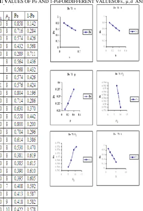
= 0.1,0.2,0.3,0.4 and b = 0.1, 0.2, 0.3, 0.4,the probability that the system is empty and the probability that the server is busy are computed and presented in table 1.The relationship between the parameters and the probability of the idealness are shown in figure 1.

Table 1: VALUES OF Po AND 1-PoFORDIFFERENT VALUESOF, µ,

a

AND b

Figure 1:Relationship between probability of Emptinessand input parameters

We have observed that when the service time parameter µ₁ increases from 5 to 11 the probability of emptiness is increasing from 0.564 to 0.576, for fixed values of  = 3,

a

= 0.1,b = 0.2, p = 0.8 andµ₂= 8.

When the service time parameter µ₂ increases from 7 to 10 the probability of emptiness is increasing from 0.408 to 0.422, for fixed values of  = 3,

a

= 0.1, b = 0.5, p = 0.8 and µ₁=10.

As the truncation parameter of the service time distribution „

a

‟ increases from 0.1 to 0.4 the probability of emptiness is increases from 0.1 to 0.4 and the probability of emptiness is increasing from 0.804 to 0.558 for fixed values of the other parameters.

As the truncation parameter of the service time distribution „b‟increases from 0.1 to 0.4 the probability of emptiness is increasing from 0.1 to 0.4 and the probability of emptiness is increasing from 0.800 to 0.530 for given values of the other parameters.

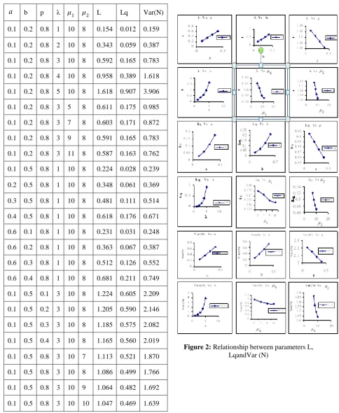
For different values of the parameters the average number of packets in the system, the average number of packets in the queue and the variance of the number of packets in the system are computed and presented in table2. The relationship between the parameters and the performance measures is shown in figure 2.

Table 2: VALUES OF L ANDLqANDVar (N)

Figure 2: Relationship between parameters L,

LqandVar (N)

From table 2 it is observed that the performance measures of the queueing model are significantly influenced by the parameters of the model. As the arrival rate  increases the average number of packets in the

a

b p λ µ₁ µ₂ L Lq Var(N)

0.1 0.2 0.8 1 10 8 0.154 0.012 0.159

0.1 0.2 0.8 2 10 8 0.343 0.059 0.387

0.1 0.2 0.8 3 10 8 0.592 0.165 0.783

0.1 0.2 0.8 4 10 8 0.958 0.389 1.618

0.1 0.2 0.8 5 10 8 1.618 0.907 3.906

0.1 0.2 0.8 3 5 8 0.611 0.175 0.985

0.1 0.2 0.8 3 7 8 0.603 0.171 0.872

0.1 0.2 0.8 3 9 8 0.591 0.165 0.783

0.1 0.2 0.8 3 11 8 0.587 0.163 0.762

0.1 0.5 0.8 1 10 8 0.224 0.028 0.239

0.2 0.5 0.8 1 10 8 0.348 0.061 0.369

0.3 0.5 0.8 1 10 8 0.481 0.111 0.514

0.4 0.5 0.8 1 10 8 0.618 0.176 0.671

0.6 0.1 0.8 1 10 8 0.231 0.031 0.248

0.6 0.2 0.8 1 10 8 0.363 0.067 0.387

0.6 0.3 0.8 1 10 8 0.512 0.126 0.552

0.6 0.4 0.8 1 10 8 0.681 0.211 0.749

0.1 0.5 0.1 3 10 8 1.224 0.605 2.209

0.1 0.5 0.2 3 10 8 1.205 0.590 2.146

0.1 0.5 0.3 3 10 8 1.185 0.575 2.082

0.1 0.5 0.4 3 10 8 1.165 0.560 2.019

0.1 0.5 0.8 3 10 7 1.113 0.521 1.870

0.1 0.5 0.8 3 10 8 1.086 0.499 1.766

0.1 0.5 0.8 3 10 9 1.064 0.482 1.692

system is increasing. Same phenomenon is observed with respective the average number of packets in the queue for the given values of the other parameters.

When the parameter µ₁ increases from 5 to 11 the average number of packet in the system is decreasing from 0.611 to 0.587 for fixed values of  = 3, µ₂= 8, b = 0.2,

a

= 0.1 and p = 0.8 Similarly the value of average number of packet in the queue is decreasing from 0.175 to 0.163 for the same changes in

µ₁when other parameters remain fixed.

When the parameter µ₂ increases from 7 to 10 the average number of packet in the system is decreasing from 1.113 to 1.047 for fixed values of  = 3, µ₁= 10, b = 0.5,

a

= 0.1 and p = 0.8 Similarly the value of average number of packet in the queue is decreasing from 0.521 to 0.469 for the same changes in µ₂

for fixed values of the other parameters.

As the truncation parameter „

a

‟ is increasing from 0.1 to 0.4 then the average number of packets in the system and the average number of packets in the queue are increasing from 0.224 to 0.618 and 0.028 to 0.176 respectively for fixed values of the other parameters.

As the truncation parameter „b‟ is increasing from 0.1 to 0.4 then the average number of packets in the system and the average numbers of packets in the queue are increasing from 0.231 to 0.681 and 0.031 to 0.211 respectively.

As the truncation parameter „p‟ is increasing from 0.1 to 0.4 then the average number of packet in the system and the average number of packet in the queue are increasing from 1.224 to 1.165 and 0.605 to 0.560 respectively for fixed values of the other parameters.

It is observed that as  increases the variance of the number of packets in the system is increasing for given values of the other parameters. When µ₁ is increasing the variance of the number of packets in the system is decreasing for fixed values of the other parameters. When the truncation parameters b is increasing the variance of the number of packets in the system is increasing. When µ₂ is increasing the variance of the number of packets in the system is decreasing for fixed values of the other parameters.

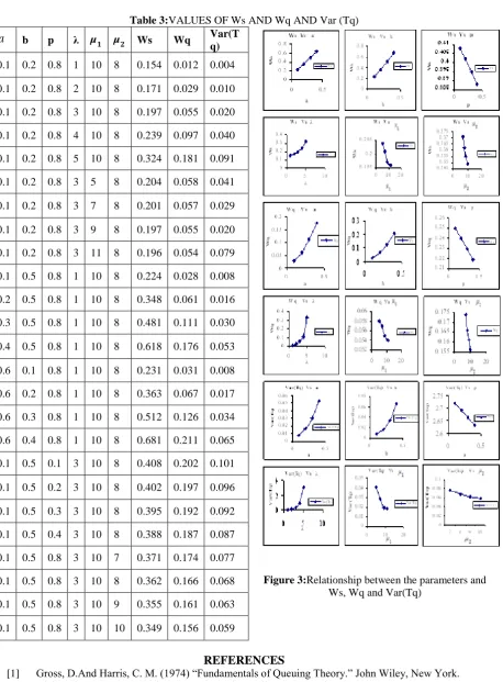
For different values of the parameterstheaverage waiting time of a packet in the system, the average waiting time of a packet in the queue and the variance of the waiting time of a packet in the queue are computed and given in the table 3. The relationship between parameters and the waiting time is shown in figure 3.

From table 3 it is observed that the model parameters have a significant influence on the waiting time of a packet in the system and in the queue. As the mean arrival rate  is increasing then the average waiting time of a packet in the queue and the average waiting time of a packet in the system are increasing when the other parameters remain fixed.

It is also observed that as the parameterµ₁ is increasing from 5 to 11 the average waiting time of a packet in the system and the average waiting time of a packet in the queue are decreasing from 0.204 to 0.196 and 0.058 to 0.054 respectively for fixed values of the other parameters.

It is also observed that as the parameter µ₂ is increasing from 7 to 10 the average waiting time of a packet in the system and the average waiting time of a packet in the queue are decreasing from 0.371 to 0.349 and 0.174 to 0.156 respectively for fixed values of the other parameters.

It is further observed that when the mean arrival rate  increases the variance of the waiting time of a packet in the system is increasing when other parameters remain fixed. Similarly when the truncation parameters

a

and b are increasing the variance of the waiting time of the packet in the system is also increasing for fixed values of the other parameters.

It is also observed that as the parameter p is increasing from 0.1 to 0.4 the average waiting time of a packet in the system and the average waiting time of a packet in the queue are decreasing from 0.408 to 0.388 and 0.202 to 0.187respectively for fixed values of the other parameters.

V1. CONCLUSION

particular cases for limiting/specific values of the parameters. This model can also be extended for non-Poison arrivals and servers vacation models.

Table 3:VALUES OF Ws AND Wq AND Var (Tq)

Figure 3:Relationship between the parameters and

Ws, Wq and Var(Tq)

REFERENCES

[1] Gross, D.And Harris, C. M. (1974) “Fundamentals of Queuing Theory.” John Wiley, New York. [2] Kleinrock,L.(1975) „Queueing Systems‟, Vol. 1, Wiley, New York.

[3] Boxima O.J. And Groenendijk W.P. (1988) „Waiting time in discrete time cyclic -service systems‟, IEEE Transactions on Communications, 36, no.2, 164 -170.

a

b p λ µ_𝟏 µ_𝟐 Ws Wq Var(T

q)

0.1 0.2 0.8 1 10 8 0.154 0.012 0.004

0.1 0.2 0.8 2 10 8 0.171 0.029 0.010

0.1 0.2 0.8 3 10 8 0.197 0.055 0.020

0.1 0.2 0.8 4 10 8 0.239 0.097 0.040

0.1 0.2 0.8 5 10 8 0.324 0.181 0.091

0.1 0.2 0.8 3 5 8 0.204 0.058 0.041

0.1 0.2 0.8 3 7 8 0.201 0.057 0.029

0.1 0.2 0.8 3 9 8 0.197 0.055 0.020

0.1 0.2 0.8 3 11 8 0.196 0.054 0.079

0.1 0.5 0.8 1 10 8 0.224 0.028 0.008

0.2 0.5 0.8 1 10 8 0.348 0.061 0.016

0.3 0.5 0.8 1 10 8 0.481 0.111 0.030

0.4 0.5 0.8 1 10 8 0.618 0.176 0.053

0.6 0.1 0.8 1 10 8 0.231 0.031 0.008

0.6 0.2 0.8 1 10 8 0.363 0.067 0.017

0.6 0.3 0.8 1 10 8 0.512 0.126 0.034

0.6 0.4 0.8 1 10 8 0.681 0.211 0.065

0.1 0.5 0.1 3 10 8 0.408 0.202 0.101

0.1 0.5 0.2 3 10 8 0.402 0.197 0.096

0.1 0.5 0.3 3 10 8 0.395 0.192 0.092

0.1 0.5 0.4 3 10 8 0.388 0.187 0.087

0.1 0.5 0.8 3 10 7 0.371 0.174 0.077

0.1 0.5 0.8 3 10 8 0.362 0.166 0.068

0.1 0.5 0.8 3 10 9 0.355 0.161 0.063

[4] Boxma,O.J., And J.W. Cohen (1998) „The M/G/1 queue with heavy-tailed service time distribution‟, IEEE J. Selected Areas Commun. 16, 749–763.

[5] Boxma, O.J,G.M.Koole,I.Mitrani (1995)„Polling models with Threshold Switching Quantative methods in parallel systems‟, 129-140.

[6] Srinivasa Rao,P.,K.SrinivasaRao and J.Lakshminarayana (2003) „Single server Poisson Queueing model with mixture of exponential service time distribution‟.Vol-15(2)M,199-204.

[7] Bunday.B.D.(1996) "An Introduction to queuing theory" John Wiley, New York.

[8] Burke. P.J. (1975) „Delays in single server queues with batch input‟, Oper.Res, 23, 830-833.

[9] Guy L.Curry, NatarajanGautam (2008) „Characterizing the departure process from a two server Markovian Queue: A Non-Renewal approach.‟ Winter Simulation Conference.

[10] Haviv, M. And Vander Wal,J. (2007) “Waiting times in queues with relative priorities,” Operations Research Letters, 35, 591-594.

[11] Hiroyuki Masuyama, Tetsuya Takine (2003)„Stationary queue length in a FIFO single server queue with service interruptions and multiple batch Markovian arrival streams‟. J.O.R.S.J, Vol-46, no.3,319-341

[12] JewgeniH.Dshalalow (1991) „A Single server queue with random accumulation level‟.J.A.M.S.A, Vol-4, No.3, 203-210.

[13] Johnson,Kotz and Balakrishnan (2004)„Continuous univeriate distributions‟ vol-1 and 2,second edition.

[14] Levy, Y. And Yechiali, U. (1975) „Utilization of idle time in an M/G/1 queueingsystem‟., Management Science 22, 202–211.

[15] Ramaswamy, R. and L.D. Servi .(1988) „The busy period of M/G/1 vacation model with Bernoulli schedule.” stochastic models, 4, 507-521.

[16] Takine T and Hesegawa T.(1992) „On M/G/1 queue with multiple vacations and gated service discipline‟, j.o.r.soc.japan-35,no.3,217-235

[17] Parthasarathy,P.R.,andK.V.Vijayashree (2002)„Fluid queues driven by a discouraged arrivals queue‟. IJMMS, Vol-24, 1509-1528

[18] MessaoudBoaunkhel,LotfiTadj (2007) „Optimal design of a bulk service queue‟, Investigacao Operacional,vol.27,131-138.

[19] K.SRINIVASA RAO, P.SURESH VARMA and Y.SRINIVAS-(2008), Interdependent Queuing Model with startup delay, Journal of Statistical Theory and Applications, Vol. 7, No. 2 pp. 219-228.

[20] Zhanyou Ma, WuyiYue, NaishuoTian (2008) „Analysis of a Geom/G/1 Queue with General Limited Service and MAVs‟.November,3,ISORA‟08, 359-368.

[21] Andreas Brandt, Manfred Brandt (2008) „Waiting times for M/systems under state-dependent processor sharing‟ Queueing Systems, Vol.59, No.3, 297-319.

[22] Ward Whitt (2006) „Fluid Models for Multiserver Queues with Abandonments‟, Operations Research, Vol.54, no.1,37-54.

[23] K.SRINIVASA RAO, G.RAMESH, and J.L.NARAYANA, (2011)- Single server Poisson queueing model with truncated exponential service times, accepted in Journal of Mathematics and Mathematical Sciences, Vol. 2.