Image Denoising Method based on Curvelet
Transform with Thresholding Functions
Neema .N Dr. M. Sasikumar
PG Student Head of Dept.
Department of Electronics & Communication Engineering Department of Electronics & Communication Engineering Marian Engineering College, Trivandrum, India Marian Engineering College, Trivandrum, India
Abstract
Visual information which is transmitted in the form of digital images is becoming a major method of communication now a day. But the main drawback in digital images is the presence of noise while their acquisition or transmission. Removing noise from digital images is a challenge for researchers. Several noise removal algorithms have been proposed till date. Choice of any denoising algorithm is application dependent and it depends upon the type of noise present in the image. Every denoising method has its own assumptions, advantages and limitations. In this paper a new image denoising method which is based on Curvelet transform is proposed. The limitations of commonly used separable extensions of one-dimensional transforms, such as the Fourier transform and wavelet transforms, in capturing the geometry of image edges are well known. Here we pursue "true" two dimensional transform, Curvelet Transform that can capture the intrinsic geometrical structure that is very important in visual information. Denoising of an image is done by Curvelet Transform with a thresholding function and the results are compared with different denoising methods. The Proposed method has the advantage of achieving a good visual quality of images while preserving the curved edges of an image. The proposed method is applied to different images such as grayscale image, color image, microscopic image, and seismic image. Experimental results show that proposed denoising technique performs better than other methods in terms of the PSNR.
Keywords: Curvelets, Discrete Wavelet Transform (DWT), Fast Discrete Curvelet Transform (FDCT) Filtering, Radon Transform, Ridgelets, Thresholding Rules, Wavelets
________________________________________________________________________________________________________
I. INTRODUCTION
Visual perception becomes an essential part of digital communication today. Because of which it is important to ensure that the transmitted data is not corrupted by any kind of unwanted signals called noise. Noises are generated due to the improper modelling of production and/or capturing system of the signal. Therefore, real signals usually contain deviations from the ideal signal that we are expecting. Image denoising is an important pre-processing task for further image processing such as edge detection or image segmentation. The main aim of any denoising algorithm is to reduce noise levels, while preserving the image characters. Presently, there are may image denoising algorithms available which are successful in denoising a noisy image, but are inefficient in attaining better signal to noise ratio and/or retaining the image features.
Image denoising in transform domain usually consist of 3 stages:
1) Transforming the noisy image to new space and finding a representation that separates the image from the noise.
2) Manipulate the coefficients in new space and keep the coefficients where SNR is high and reduce the coefficient where SNR is low.
3) Transforming the manipulated coefficients back to original space.
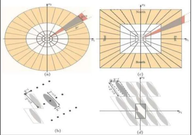
Fig. 1: Representation of curved singularities using (a) curvelets (b) wavelets
One of the primary tasks in computer vision is to extract features of an image or a sequence of images. The features may be points, lines, edges, and textures. A given feature is characterized by its position, direction, scale, and other property parameters. The most common technique, used in early vision for extraction of such features, is the linear filtering, which is also reflected in models used in biological visual systems, i.e., human visual motion sensing. Objects at different scales can arise from distinct physical processes. This leads to the use of scale-space filtering and multiresolution wavelet transform in this field. An important motivation for computer vision is to obtain directional representations that capture anisotropic lines and edges while providing sparse decompositions. To overcome the missing directional selectivity of conventional two-dimensional (2-D) discrete wavelet transforms (DWTs), a multiresolution geometric analysis (MGA), named curvelet transform, was proposed . In the 2-D case, the curvelet transform allows an almost optimal sparse representation of objects with singularities along smooth curves. Unlike the isotropic elements of wavelets, the needle-shaped elements of the curvelet transform possess very high directional sensitivity and anisotropy (see Fig 1 for the 2-D case). Such elements are very efficient in representing line-like edges. Recently, the curvelet transform has been extended to three dimensions. The theoretic concept of curvelets is easy to understand, but how to achieve the discrete algorithms for practical applications is challenging.
II. LITERATURE REVIEW
Noise will be unavoidable during image acquisition process and denoising is an essential step to improve the image quality. Image denoising involves the manipulation of the image data to produce a visually high quality image. Finding efficient image denoising methods is still valid challenge in image processing. There are various noise reduction techniques used for removing noise. Most of the standard algorithms use to denoise the noisy image and perform the individual filtering process which reduces the noise level. But the image is either blurred or over smoothed due to the lose of edges. Noise reduction is used to remove the noise without losing detail contained in the images.
Image Denoising With The Contourlet Transform.
Image denoising involves transform domain coefficient manipulation followed by the inverse transform. This approach is highlighted by recently-developed methods that model the inter-coefficient dependencies. However, these methods operate on the transform domain error rather than on the more relevant image domain one. In [11] a novel denoising method, based on the Basis Pursuit Denoising (BPDN) method is done. This method combines the image domain error with the transform domain dependency structure, resulting in a general objective function, applicable for any wavelet like transform called Contourlet Transform (CT), a relatively new transform designed to sparsely represent images. It is well known that many signal processing tasks, e.g. compression, denoising, feature extraction and enhancement, benefit tremendously from having a parsimonious representation of the signal at hand and it improves the representation sparsity of images over the Wavelet Transform (WT). The main feature of these transforms is the potential to efficiently handle 2-D singularities, i.e. edges, unlike wavelets which can deal with point singularities exclusively.
Image denoising using Wavelet Transform.
Wavelet transform is a mathematical function that analyzes the data according to scale or resolution. In [7] noise reduction using wavelets is performed by first decomposing the noisy image into wavelet coefficients i.e. approximation and detail coefficients. Then, by selecting a proper thresholding value the detail coefficients are modified based on the thresholding function. Finally, the reconstructed image is obtained by applying the inverse wavelet transform on modified coefficients.
with large number of zero coefficients. This leads to a smooth signal. So much attention must be paid while selecting an optimal threshold.
Multilevel Threshold Based Image Denoising in Curvelet Domain.
A multilevel thresholding technique for noise removal in curvelet transform domain which uses cycle-spinning is implemented in [5]. Cycle spinning for denoising is a simple and efficient method that can be applied to a shift variant transform for signal denoising. The data is shifted, denoised and unshifted. For the discrete curvelet transform the shift length of rows and columns depends on the block size. Most of uncorrelated noise gets removed by thresholding curvelet coefficients at lowest level, while correlated noise gets removed by only a fraction at lower levels, so we used multilevel thresholding on curvelet coefficients. The threshold in the proposed method depends on the variance of curvelet coefficients, the mean and the median of absolute curvelet coefficients at a particular level which makes it adaptive in nature. Wavelet and other frequency transforms are widely used for denoising, but they suffer from shift and rotation sensitivity, as well as they are poor in directionality. Curvelet transform are more suitable for detection of directionality properties as they provide optimally sparse representations of objects which display curve punctuated smoothness except for discontinuity along a general curve with bounded curvature
Image Denoising using Adaptive Thresholding in Framelet Transform Domain.
Wavelet transform has proved to be effective in noise removal and also reduce computational complexity, better noise reduction performance. Apply discrete wavelet transform (DWT) which transforms the discrete data from time domain into frequency domain. Wavelet denoising attempts to remove the noise present in the imagery while preserving the image characteristics, regardless of its frequency content. Many of the wavelet based denoising algorithms use DWT (Discrete Wavelet Transform) in the decomposition stage which is suffering from shift variance. To overcome this, in [8] proposed a denoising method which uses Framelet transform to decompose the image and performed shrinkage operation to eliminate the noise . The idea is to transform the data into the Framelet basis, for example shrinkage followed by the inverse transform.
III. THEORETICAL BACKGROUND
Curvelets are a non-adaptive technique for multi-scale object representation. Being an extension of the wavelet concepts, they are becoming popular in similar fields, namely in image processing and scientific computing. Curvelet transform is a multi-scale geometric wavelet transforms, can represent edges and curves singularities much more efficiently than traditional wavelet. Curvelet combines multiscale analysis and geometrical ideas to achieve the optimal rate of convergence by simple thresholding. Multi-scale decomposition captures point discontinuities into linear structures. Curvelets in addition to a variable width have a variable length and so a variable anisotropy. The length and width of a curvelet at fine scale due to its directional characteristics is related by the parabolic scaling law:
Width (length) 2
Curvelets partition the frequency plan into dyadic coronae that are sub partitioned into angular wedges displaying the parabolic aspect ratio as shown in Fig 2 .
which the window isolates the frequency near trapezoidal wedge such as the one shown in gray (d)The wrapping transformation the dashed line shows the same trapezoidal wedge as in b. The parallelogram contains this wedge and hence the support of the curvelet.
Curvelets at scale 2-k ,are of rapid decay away from a “ridge” of length 2-k/2 and width 2-k and this ridge is the effective support. The discrete translation of curvelet transform is achieved using wrapping algorithm. The curvelet coefficients Ck for each scale and angle is defined in Fourier domain
Ck(r,) = 2-3k/4R (2-kr) A (2(k/2)/2𝝅.𝜽) (1)
Where Ck in this equation represents polar wedge supported by the radial(R) and angular (A) windows.
Curvelets are based on multiscale ridgelets combined with a spatial bandpass filtering operation to isolate different scale. Like ridgelets, curvelets occur at all scales, locations, and orientations. However, while ridgelets all have global length and variable widths, curvelets in addition to a variable width have a variable length and so a variable anisotropy. The length and width at fine scales are related by a scaling law width= length2 and so the anisotropy increases with decreasing scale like a power law. Recent work shows that thresholding of discrete curvelet coefficients provide near optimal N–term representations of otherwise smooth objects with discontinuities along curves. Thus for understanding curvelet, we should have the knowledge about ridgelet and radon transform.
Continuous Ridgelet Transform
The ridgelet transform of two-dimensional function f(x,y) allows the sparse representation of both smooth function and of straight edges by superposition of ridgelet function. For every L2 (R2) we get its ridgelet coefficients R
f (a,b,θ) by a inner product with the frame like function Ψa,b,θ (x) which is a wavelet in transverse orientation constant along the line
x1cosθ + x2sinθ = constant.
For every a>0, each b ϵ R and each θ ϵ [0, 2π), the bivariate ridgelet Ψa,b,θ is given by
(2)
This function is constant along the lines x1cosθ +x2 sinθ =constant.Transverse to these ridges it is a wavelet. Given an integrable bivariate function f(x), the ridgelet coefficients by
(3) The reconstruction formulae is given as
(4)
Furthermore, this formula is stable as one has a Parseval relation is given by
(5)
Hence, much like the wavelet or Fourier transforms, the above identity expresses the fact that one can represent any arbitrary function as a continuous superposition of ridgelets.
Radon Transform
A basic tool for calculating ridgelet coefficients is to view ridgelet analysis as a form of wavelet analysis in the Radon domain.
The Radon transform of an object f is the collection of line integrals indexed by (θ,t) ϵ [0,2π) €×R.
(6)
Where δ is the Dirac distribution. The ridgelet coefficients Rf(a,b,θ) of an objects f are given by analysis of the Radon transform via
(7)
Hence, the ridgelet transform is precisely the application of a one-dimensional (1-D) wavelet transform to the slices of the Radon transform where the angular variable θ is constant and t is varying.
Discrete Curvelet Transform of Continuum Function
The discrete curvelet transform of a continuum function f(x1,x2) makes use of a dyadic sequence of scales, and a bank of filters with the property that the pass band filter with the property that the pass band filter
is concentrated near the frequencies. In wavelet theory, one uses decomposition into dyadic subbands .In contrast, the subbands used in the discrete curvelet transform of continuum functions have the nonstandard form. This is nonstandard feature of the discrete curvelet transform well worth remembering.
Digital Realization
rather obvious and direct. However, experience shows that one modification is that, rather than merging the two the two dyadic subbands and as in the theoretical work, in the digital application, leaving these subbands separate, applying spatial partitioning to each subband and applying the ridgelet transform on each subband separately led to improved visual and numerical results. A trous subband filtering algorithm is especially well-adapted to the needs of the digital curvelet transform. The algorithm decomposes a n by n image as a superposition of the form
I(X, Y) = C(X, Y) + ∑Jj=1w(x, y) (8)
where C(X,Y) is a coarse or smooth version of the original image and w represents “the details of ” at scale 2-j . Thus, the algorithm outputs J+1subband arrays of size n*n . [The indexing is such that, here, j=1 corresponds to the finest scale (high frequencies).
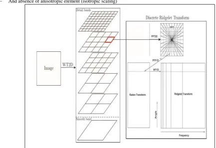
The basic process of the digital realization for curvelet transform [Fig 3] is given as follows sub-band decomposition : The object is decomposed into subbands .
Smooth Partitioning : Each subband is smoothly windowed into squares of an appropriate scale (of side length~2-j ) . Renormalization : Each resulting square is renormalized to unit scale.
Ridgelet Analysis : Each square is analyzed via the DRT .
Most successful approaches related with the discrete curvelet transform are hybrid methods, where curvelets are combined with another technique for image processing. These methods usually can exploit the ability of the curvelet transform to represent curve-like features. Recent work shows that thresholding of discrete curvelet coefficients provide near optimal N–term representations of otherwise smooth objects with discontinuities along curves. The unique mathematical property for representing curved singularities in a non-adaptive manner makes the Curvelet transform a higher-dimensional generalization of wavelets.
The major advantage of the curvelet transforms compared to the wavelet is that the edge discontinuity is better approximated by curvelets than wavelets. Curvelets can provide solutions to the limitations that are apparent in wavelet transform and summarized as follows:
Curved singularity representation,
Limited orientation (Vertical, Horizontal and Diagonal) And absence of anisotropic element (isotropic scaling)
Fig. 3: Flow Chart Of First Generation Discrete Curvelet Transform .The figure illustrates the decomposition of the original image into sub-bands followed by the spatial partitioning of each sub-band. the ridgelet transform is then applied to each block.
IV. PROPOSED DENOISING METHOD
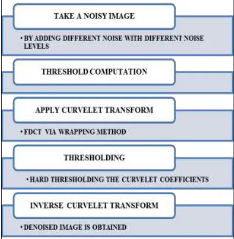
curvelet transform of noisy image is computed. Then by hard thresholding the curvelet coefficients and taking the inverse curvelet transform denoised image is obtained.
Fig. 4: Block Diagram of the Proposed Denoising Method
Parameter Estimation for Threshold Value
The threshold value is selected at 3*sigma_jl for all but the finest scale where it is set at 4*sigma_jl; here sigma_jl is the noise level of a coefficient at scale j and angle (equal to the noise level times the l2 norm of the corresponding curvelet. There are many ways to compute the sigma_jl 's, e.g. by calculating the norm of each individual curvelet and in this method do an exact computation by applying a forward curvelet transform on the image which contains a delta function at its center.
Thresholding
Thresholding is a simple non-linear technique, which operates on one curvelet coefficient at a time. Each coefficient is thresholded by comparing against threshold which is calculated. If the coefficient is smaller than the threshold it is set to zero otherwise it is modified. Replacing the noisy coefficients by zero and inverse transform on the result provide reconstruction with the essential image characteristics which is free from noise and minimum mean squared error (MSE).
There are two primary thresholding methods: hard thresholding and soft thresholding. The hard thresholding operator is defined as
The soft thresholding operator is defined as
Curvelet Transform
Digital curvelet transform can be implemented in 2 ways (FDCT via USFFT and FDCT via wrapping) which differs by spatial grid which is used to translate the curvelets at each scale and angle. In this thesis a newly constructed and improved version of curvelet transform called Fast Discrete Curvelet Transform (FDCT) is implemented. This new technique is simpler, less redundant and faster than the original curvelet transform which is based on ridgelets. This transform is constructed using parabolic scaling law, tight framing and wrapping.
There are two implementations of FDCT :
unequally spaced Fast Fourier transforms (USFFT) wrapping function
Wrapping Based Curvelet
By applying FDCT via wrapping for multiscale analysis the image is decomposed into a series of disjoint subbands, which are composed of the curvelet coefficients .The subbands are mainly classified as three groups , namely the coarse scale ,detail scale and fine scale .The innermost scale is the coarse scale composed of the low frequency curvelet coeeficients, which provides the general information and key energy present in an image. The outermost scale is the finescale containing the high frequency curvelet coefficients which gives the detail information and edge feature of the image. The remaining scales are classified as the detail scales which contains the middle high frequency curvelet coefficients, which also provides the edge feature information of the image. Then by thresholding the curvelet coefficients and taking inverse transform denoising is done
V. RESULTS AND DISCUSSIONS
This section presents the effect of the proposed method for removal of noise in standard images like 8-bit grayscale Lena image as well as for Color image Peppers and other test images like MRI image ,Seismic image, and microscopic image. The noisy images are simulated by adding different noises with different noise levels on the original images. The types of noise considered in this paper were Gaussian, Salt and Pepper and Poisson noise. FDCT via wrapping is used for implementation .The results of the proposed approach is introduced in a comparison form as FDCT with hard thresholding and FDCT with soft thresholding.
Performance Evaluation
The performance of the method is illustrated by both the quantitative and qualitative performance measure. The qualitative measure is the visual quality of the resulting image. The peak signal to noise ratio (PSNR) is used as quantitative measure. PSNR is an engineering term for the ratio between the maximum possible power of a signal and the power of corrupting noise that affects the fidelity of its representation. Because many signals have a very wide dynamic range,
PSNR is usually expressed in terms of the logarithmic decibel scale. PSNR is computed using the equation
PSNR = 10log10(
255 ∗ 255
MSE )
For an 8 bit image .Here 255 is the maximum grayscale value and MSE is calculated by
MSE = 1
mn∑ ∑ [I(j, y) − K(i, j)]
n−1 j=0 m−1
i=0 2
Where I and K are the original and denoised images respectively.
Implementation Results
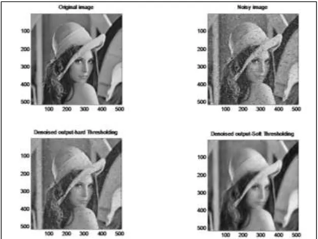
The visual quality of the denoised image obtained using the proposed method is found to be superior to other well known denoising methods. The denoised image was found to have minimal distributing artifacts and the curved edges are almost preserved.
Fig. 6: Denoising results of 512 x 512 Lena image under Salt & pepper noise with noise density .05
Fig. 7: Denoising results of 512 x 512 Lena image under Poisson noise with noise density .05 Table – 1
PSNR Values for Denoised Grayscale Image Using Proposed Method TYPE OF THRESHOLD TYPE OF NOISE NOISE LEVEL PSNR
HARD
GAUSSIAN
30 31.1909
60 26.474
80 25.3208
SALT AND PEPPER
0.02 24.9274
0.03 23.4387
0.09 22.09
POISSON 0.5 32.1868
2.5 32.178
SOFT
GAUSSIAN
20 28.1534
60 24.0628
80 23.164
SALT AND PEPPER
0.02 26.716
0.03 26.273
0.09 24.417
POISSON
0.5 32.2716
1 32.2907
2.5 32.2754
Fig. 8: PSNR Plot Of Denoised Lena Image
In the case of grayscale image PSNR values obtained are better for curvelet transform with hard thresholding under Gaussian and Poisson noise. The visual quality are also improved while preserving curved edges .
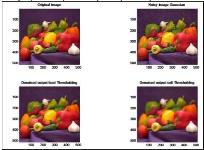
Fig. 10: Denoising results of 512 x 512 Peppers image under Salt & Pepper noise with noise density .05
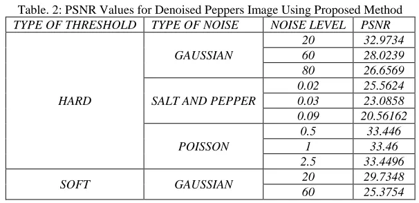
Fig. 11: Denoising results of 512 x 512 Peppers image under Poisson noise with noise density .05 Table. 2: PSNR Values for Denoised Peppers Image Using Proposed Method
TYPE OF THRESHOLD TYPE OF NOISE NOISE LEVEL PSNR
HARD
GAUSSIAN
20 32.9734
60 28.0239
80 26.6569
SALT AND PEPPER
0.02 25.5624
0.03 23.0858
0.09 20.56162
POISSON
0.5 33.446
1 33.46
2.5 33.4496
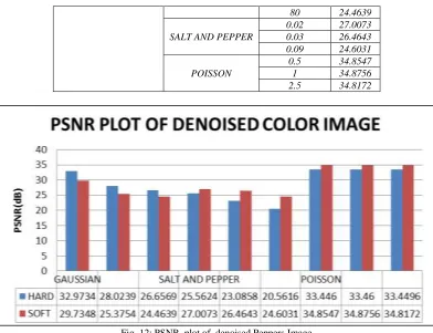
SOFT GAUSSIAN 20 29.7348
80 24.4639
SALT AND PEPPER
0.02 27.0073
0.03 26.4643
0.09 24.6031
POISSON
0.5 34.8547
1 34.8756
2.5 34.8172
Fig. 12: PSNR plot of denoised Peppers Image
In the case of color image PSNR values obtained are better for curvelet transform with hard thresholding under Gaussian noise but in the case of salt and pepper and Poisson noise it perform well with soft thresholding. The visual quality are also improved while preserving curved edges .Apart from the standard natural images, this method was implemented on microscopic image ,seismic image .The proposed method showed significant denoising in all these test images. This proves the utility of the proposed method in denoising any kind of image available.
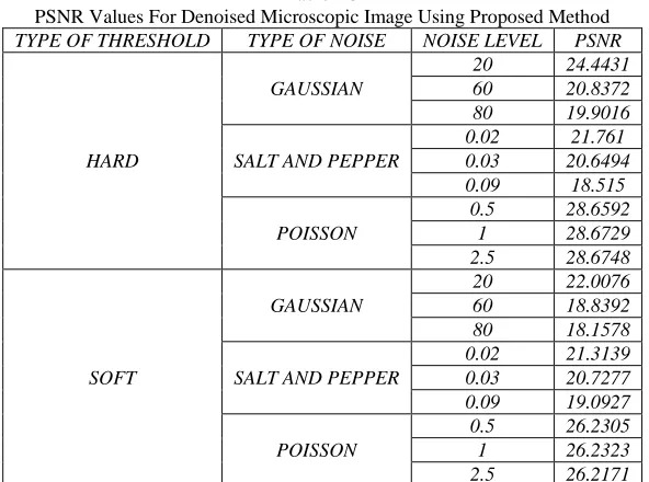
Fig. 14: Denoised Microscopic Image under Salt & Pepper Noise with Noise Density 0.05 Table – 3
PSNR Values For Denoised Microscopic Image Using Proposed Method
TYPE OF THRESHOLD TYPE OF NOISE NOISE LEVEL PSNR
HARD
GAUSSIAN
20 24.4431
60 20.8372
80 19.9016
SALT AND PEPPER
0.02 21.761
0.03 20.6494
0.09 18.515
POISSON
0.5 28.6592
1 28.6729
2.5 28.6748
SOFT
GAUSSIAN
20 22.0076
60 18.8392
80 18.1578
SALT AND PEPPER
0.02 21.3139
0.03 20.7277
0.09 19.0927
POISSON
0.5 26.2305
1 26.2323
Fig. 15: PSNR Plot Of Denoised Microscopic Image
In the case of microscopic image PSNR values obtained are better for curvelet transform with hard thresholding under Gaussian and Poisson noise.
Fig. 17: Denoised Microscopic Image Under Poisson Noise with Noise Density 0.05
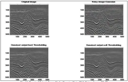
Fig.18: Denoised Seismic Image Under Poisson Noise with Noise Density .05 Table – 4
PSNR Values For Denoised Seismic Image Using Proposed Method
TYPE OF THRESHOLD TYPE OF NOISE NOISE LEVEL PSNR
HARD
GAUSSIAN
20 27.4944
60 21.2557
80 19.992
SALT AND PEPPER
0.02 23.6831
0.03 22.2583
0.09 20.0599
POISSON 0.5 30.1975
2.5 30.1983
SOFT
GAUSSIAN
20 23.1963
60 18.908
80 18.232
SALT AND PEPPER
0.02 22.731
0.03 21.862
0.09 19.604
POISSON
0.5 34.8547
1 34.8756
2.5 34.8172
Fig. 19: PSNR Plot of Denoised Seismic Image
In the case of seismic image PSNR values obtained are better for curvelet transform with hard thresholding under Gaussian and Poisson noise and with soft thresholding under Poisson noise.
Comparative Study Outcomes
The proposed method not only has a superior visual quality but also excels in terms of evaluation parameter ie, PSNR values obtained by the proposed method are also improved. The PSNR values obtained by the proposed method were plotted along with other denoising methods subject to same noise conditions. The plot is as shown in Fig 6.23.The results of the proposed method were compared with other transform domain techniques like Wavelet domain, and Contourlet domain transform. The resulting denoised images have higher visual quality than other methods Table 5 shows the image quality assessment for image with Gaussian noise of 𝜎 = 30 𝑑𝐵.
Table – 5
PSNR values for different domain denoising techniques for Gaussian noise of 𝜎 = 30 𝑑𝐵 Image Wavelet Domain Denoising Contourlet domain denoising Proposed method
Lena 28.7156 30.6254 31.1019
Peppers 27.6492 30.5679 31.1631
Fig. 20: PSNR plot of different image denoising method in comparison with the proposed method under Gaussian noise VI. CONCLUSION
The primary goal of noise reduction is to remove the noise without losing much detail contained in an image. To achieve this goal, a mathematical function known as curvelet transform is used. The experimental results show that the curvelet transform with hard thresholding gives better results/performance than other denoising methods in terms of PSNR value. Curvelet transform denoised different images under different noises and this denoising method performs well under Gaussian and Poisson noise with hard thresholding in terms of PSNR value. The graph shows a decrease in PSNR value as the sigma value increases, which is natural because, as the noise increases the signal to noise ratio is expected to decrease. It does not effectively remove salt and pepper noise but it recovers curves and edges. The visual quality of the denoised images obtained are also improved using Curvelet Transform with hard thresholding.
ACKNOWLEDGMENT
I would like to express my special gratitude and thanks for giving me attention and time.
REFERENCES
[1] A. Anilet Bala, Chiranjeeb Hati and CH Punith, ‘’Image Denoising Method Using curvelet Transform and Wiener Filter’’ International Journal of Advanced Research in Electrical, Electronics and Instrumentation Engineering (An ISO 3297: 2007 Certified Organization) Vol. 3, Issue 1, January 2014 [2] Jianwei Ma and Gerlind Plonka “The Curvelet Transform, A review of recent applications” IEEE Signal processing Magazine March 2010
[3] Usama Sayed, M. A. Mofaddel, W. M. Abd-Elhafiez and M. M. Abdel-Gawad “Image Object Extraction Based on Curvelet Transform” Applied Mathematics & Information Sciences ,An International Journal Appl. Math. Inf. Sci. 7 No. 1, 133-138 (2013)
[4] Vishal Garg, Nisha Raheja “Image Denoising Using Curvelet Transform Using Log Gabor Filter” International Journal of Advanced Research in Computer Engineering & Technology Volume 1, Issue 4, June 2012.
[5] Binh NT, Khare A Nguyen Thanh Binh and Ashish Khare. “Multilevel threshold based image denoising in curvelet domain.” Journal of computer science and technology 25(3): 632–640 May 2010.
[6] JIANG Taoa,Zhaoxinb “Research and application of image denoising method based on curvelet transform”The International Archives Of The Photogrammetry, Remote Sensing And Spatial Information Sciences. Vol. XXXVII. Part B2. Beijing 2008.
[7] Jappreet Kaur, Manpreet Kaur, Poonamdeep Kaur, Manpreet Kaur4 “Comparative Analysis of Image Denoising Techniques International Journal of Emerging Technology and Advanced Engineering”Website: www.ijetae.com (ISSN 2250-2459, Volume 2, Issue 6, June 2012).
[8] S.Sulochana, R.Vidhya “Image Denoising using Adaptive Thresholding in Framelet Transform Domain” (IJACSA) International Journal of Advanced Computer Science and Applications, Vol. 3, No. 9, 2012 .
[9] M. Antonini, M. Barlaud, P. Mathieu, I. Daubechies, ―Image coding using wavelet transform", IEEE Trans. Image Processing, Vol. 1, pp. 205- 220, 1992. [10] Jean-Luc Starck, Emmanuel J. Candès, and David L. Donoho,‖ The Curvelet Transform for Image Denoising‖. IEEE Transactions on image processing, vol.
11, no. 6, June 2002.
[11] Boaz Matalon, Michael Zibulevsky, and Michael Elad, “Image denoising with the Contourlet transform,” in Proceedings of the SPIE conference wavelets, July 2005, vol. 5914.
[12] E. Candès, L. Demanet, D. Donoho, and L. Ying, “Fast discrete curvelet transforms,” Multiscale Model. Simul., vol. 5, no. 3, pp. 861–899, 2006.
[13] H. Shan, J. Ma, and H. Yang, “Comparisons of wavelets, contourlets, and curvelets for seismic denoising,” J. Appl. Geophys., vol. 69, no. 2, pp. 103–115, 2009.