Multiresolution Subband Blind Source
Separation: Models and Methods
Hongwei Li1, Rui Li2, Fasong Wang1
1.School of Mathematics and Physics, China University of Geosciences, Wuhan 430074, P.R.China Email: [email protected], [email protected]
2.School of Sciences, Henan University of Technology, Zhengzhou 450052, P.R.China Email: [email protected]
Abstract—The goal of this paper is to review the multiresolution subband Blind Source Separation (MRSBSS) methods, classify them into different categories, and identify new trends. After the perspective of MRSBSS is briefly presented, the general and detailed definition of the MSBSS model is given, the relationships among BSS, Independent Component Analysis (ICA) and MRSBSS method are discussed simultaneously. Then, the state-of-the-art MRSBSS algorithms: adaptive filter based method and sparsity based multiscale ICA method are constructed and overviewed in detail from different theory base. The paper concludes by discussing the impact of multiresolution subband on BSS research and outlining potential future research directions and applications.
Index Terms—Independent Component Analysis(ICA), Blind Source Separation(BSS), Independent Subspace Analysis(ISA), Subband; Multiresolution, Wavelet; Wavelet Packets
I. INTRODUCTION
Standard Blind Source Separation (BSS) model and methods have been successfully applied to many areas of science [1-2]. The basic BSS model assumes that the observed signals are linear superposition’s of underlying hidden source signals. Most of the BSS algorithms are based on the independent assumption of the source signals which is called Independent Component Analysis (ICA). Despite the success of using standard ICA in many applications, the basic assumptions of ICA may not hold hence some caution should be taken when using standard ICA to analyze real world problems, especially in biomedical signal processing and image processing. In fact, by definition, the standard ICA algorithms are not able to estimate statistically dependent original sources, that is, when the independence assumption is violated.
Among many extensions of the basic ICA model, several researchers have studied the case where the source signals are not statistical independent, we call these models Dependent Component Analysis (DCA) model as a whole. The first extended DCA model is the Multidimensional Independent Component Analysis (MICA) model[3], which is a linear generative model as ICA. In contrast to ordinary ICA, however, the
components (responses) are not assumed to be all mutually independent. Instead, it is assumed that the source signals can be divided into couples, triplets, or in general i-tuples, such that the source signals inside a given i-tuple may be dependent on each other, but dependencies among different i-tuples are not allowed. Based on this basic extension of the ICA model, there have emerged lots of DCA models and corresponding algorithms, such as independent subspace analysis[4], variance dependent BSS[5], topographic ICA[6], and tree-dependent component analysis[7], subband decomposition ICA[8], maximum non-Gaussianity method [9-10], spectral decomposition method[11], time-frequency method[12-13].
In these methods, the subband decomposition ICA[8] method can be naturally extended and generalized to multiresolution subband BSS(MRSBSS) which relaxes considerably the assumption regarding mutual independence of primarily sources. The more powerful assumption is non-independent of the sources decomposition coefficients, when the signals are properly represented or transformed. Multiresolution analysis (MRA) will show how discrete signals are synthesized by beginning with a very low resolution signal and successively adding on details to create higher resolution versions, ending with a complete synthesis of the signal at the finest resolution. This is known as. In these transformed fields, the coefficients do not necessarily have to be linearly independent and, instead, may form an overcomplete set (or dictionary), for example, wavelet packets, stationary wavelets, time-frequency transformations. The key idea in this approach is the assumption that the wide-band source signals or their transformations are dependent, however some narrow band subcomponents are independent. In other words, we assume that each unknown source can be modeled or represented as a sum of narrow-band sub-signals (sub-components)[2]:
,1 ,2 ,
( ) ( ) ( ) ( )
i i i i K
purpose at hand. The subband signals can be ranked and processed independently. Let us assume that only a certain set of sub-components is independent. Provided that for some of the transformation subbands (at least one) of all sub-components, say
, 1, , ;
{1, , }
ip
s i
=
L
N p
∈
L
K
, are mutually independent or temporally decorrelated, then we can easily estimate the mixing or separating system (under condition that these subbands can be identified by some a priori knowledge or detected by some self-adaptive process) by simply applying any standard BSS/ICA algorithm, however not for all available raw sensor data but only for suitably preprocessed (band pass filtered) sensor signals. Such explanation can be summarized as follows.In one of the most simplest cases, source signals can be modeled or decomposed into their low- and high- frequency sub-components:
, ,
( ) ( ) ( )
i i H i L
s t =s t +s t (1.2) In practice, the high-frequency sub-components
, ( )
i H
s t are often found to be mutually independent. In such a case in order to separate the original sources
( )
i
s t , we can use a High Pass Filter (HPF) to extract high frequency sub-components and then apply any standard ICA algorithm to such preprocessed sensor (observed) signals. In the preprocessing stage, more sophisticated methods, such as block transforms, multi-rate subband filter bank or wavelet transforms, can be applied.
Definition 1.6[2] (Multiresolution Subband Blind Signal Separation: MRSBSS) The MRSBSS can be formulated as a task of estimation of the mixing matrix on the basis of suitable multiresolution subband decomposition of sensors signals and by applying a classical BSS method(instead for raw sensor data) for one or several pre-selected subbands for which source sub-components are least dependent.
II. MULTIRESOLUTION SUBBAND BSSMODEL
A. BSS model
Let us denote the N source signals by the vector
1
( ) ( ( ), , ( ))T N t = s t s t
s L , and the observed signals by
1
( ) ( ( ), , ( ))T M t = x t x t
x L . Now the mixing can be
expressed as
( )t = ( )t + ( )t
x As n , (2.1)
where the matrix [ ] M N
ij a R ×
= ∈
A collects the mixing
coefficients. No particular assumptions on the mixing coefficients are made. However, some weak structural assumptions are often made: for example, it is typically assumed that the mixing matrix is square, that is, the number of source signals equals the number of observed signals (M =N), the mixing process A is defined by an even-determined (i.e. square) matrix and, provided that it is non-singular, the underlying sources can be estimated by a linear transformation, which we will
assume here as well. If M >N, the mixing process A
is defined by an over-determined matrix and, provided that it is full rank, the underlying sources can be estimated by least-squares optimization or linear transformation involving matrix pseudo-inversion. If
M <N , then the mixing process is defined by an under-determined matrix and consequently source estimation becomes more involved and is usually achieved by some non-linear technique. For technical simplicity, we shall also assume that all the signals have zero mean, but this is no restriction since it simply means that the signals have been centered. ( ) ( ( ), ,1 ( ))T
M t = n t n t
n L is a vector of
additive noise. The problem of BSS is now to estimate both the source signals s tj( ) and the mixing matrix A
based on observations of the x ti( ) alone [1-2].
The task of BSS is to recover the original signals from the observations x( )t without the knowledge of A
nor s( )t . Let us consider a linear feed forward memoryless neural network which maps the observation
( )t
x to y( )t by the following linear transform ( )t = ( )t = ( )t
y Wx WAs ,
where [ ] n m
ij w R ×
= ∈
W is a separating matrix,
1
( ) ( ( ), , ( ))T n t = y t y t
y L is an estimate of the possibly
scaled and permutated vector of s( )t and also the network output signals whose elements are statistically mutually independent, so that the output signals y( )t are possibly scaled estimation of source signals s( )t .
There are two indeterminacies in ICA: (1) scaling ambiguity; (2) permutation ambiguity. But this does not affect the application of ICA, because the main information of the signals is included in the waveform of them. Under this condition, Comon proved that the separated signals y ti( ) , i=1, 2, ,L n are mutually independent too [14].
Theorem 1 Let s be a random vector with independent components, of which at most one is Gaussian. Let C is an invertible matrix andy Cs= , then the following two properties are equivalent:
(1) The components yi are mutually independent; (2) C Q= Λ,where Q is a permutation matrix and Λ is a nonsingular diagonal matrix.
To cope with ill-conditioned cases and to make algorithms simpler and faster, a linear transformation called prewhitening is often used to transform the observed signals x to
x Vx
%
=
such that[
T]
B MRSBSS Model
The assumption of statistical independence of the source components
s t
i( )
leads itself to ICA and justified by the physics of many practical applications. A more powerful assumption is non-independent of the decomposition coefficients when the signals are properly represented[15-18]. Suppose that eachs t
i( )
have a transformed representation of its decomposition coefficientsc
ik obtained by means of the set of representation functions{
ϕ
k( ),
t k
=
1, ,
L
K
}
:1
( )
K( )
i ik kk
s t
c
ϕ
t
=
=
∑
(2.2)The functions
ϕ
k( )
t
are called atoms or elements of the representation space that may constitute a basis or a framework. These elements{
ϕ
k( ),
t k
=
1, ,
L
K
}
do not have to be linearly independent and, instead, may be mutually dependent and form an overcomplete set (or dictionary), for example, wavelet-related dictionaries: wavelet packets, stationary wavelets, etc. [19-20]. The corresponding representation of the mixtures x( )t , according to the same signal dictionary, is:1
( )
K( )
i ik kk
x t
d
ϕ
t
=
=
∑
(2.3)1
( )
K( )
i ik kk
n t
e
ϕ
t
=
=
∑
(2.4)where
d
ik ande
ik are the decomposition coefficients of the mixtures and noises.Let us consider the case wherein the subset of functions
{
ϕ
k( ),
t k
∈Ω
}
is constructed from the mutually orthogonal elements of the dictionary. This subset can be either complete or undercomplete.Define vectors
{ ,
d
ll
∈Ω
}
,{ ,
c
ll
∈Ω
}
and{ ,
e
ll
∈Ω
}
to be constructed from the k-th coefficients of mixtures, sources and noises, respectively. From (2.1), (2.2)-(2.4), and using the orthogonality of the subset of functions{
ϕ
k( ),
t k
∈Ω
}
, the relation between the decomposition coefficients of the mixtures and of the sources isl = l+ l
d Ac n (2.5) Note, that the relation between decomposition coefficients of the mixtures and the sources is exactly the same relation as in the original domain of signals. Then, estimation of the mixing matrix and of sources is performed using the decomposition coefficients of the mixtures dl instead of the mixtures x( )t .
The property of coefficients in the transform domain often yields much better source separation than standard BSS methods, and can work well even with more sources than mixtures. In many cases there are distinct groups of
coefficients, wherein sources have different statistical properties. The proposed multiresolution, or multiscale, approach to the BSS is based on selecting only a subband or subset of features, or coefficients,
D
=
{ ,
d
ll
∈Ω
}
, which is best suited for separation, with respect to the coefficients and to the separability of sources’ features.So, for MRSBSS model, in order to estimating the source signals, it is very important to choose the form of the transformation and the approach to select the optimal subband or subset of the coefficients. In the next section, we will review some algorithms to solve the MRSBSS model using different transformations and subband selection methods.
III. MRSBSSALGORITHMS
Different approaches to transformations of the source signals and various methods to choose the optimal subset of the coefficients can result in a set of MRSBSS algorithms. The whole procedure of the MRSBSS, from mixing to separating, is described in figure 1. In this section, we will give an overview to these approaches. A Adaptive Filter Based Method
Subband decomposition ICA(SDICA) [8,21-23], an extension of ICA, assumes that each source is represented as the sum of some independent subcomponents and dependent subcomponents, which have different frequency bands. SDICA model can considerably relax the assumption regarding mutual independence between the original sources by assuming that the wide-band source signals are generally dependent but some narrow-band subcomponents of the sources are independent.
1
s
∈
R
2
s
∈
R
M
N
s
∈
R
1
x
∈
R
2
x
∈
R
M
M
x
∈
R
1
y
∈
R
2
y
∈
R
M
N
y
∈
R
A
W
M N× ∈
A R W R∈ M N×
( )t n
M M× ∈ V R
V
1
x
%
∈
R
2
x
%
∈
R
M
M
x
%
∈
R
k
:
k R→R
1
ˆ
x
∈
R
2
ˆ
x
∈
R
M
ˆ
Mx
∈
R
Figure 1. The whole mixing-separation procedure of MRSBSS, where [ , ,1 ]T N N
s s
= ∈
s L R is the hidden source signals;
1
[ , , ]T M
M
x x
= ∈
x L R is the observation and x( )t =As( )t ; [ , ,1 ]T M M
x x
= ∈
x% % L % R is the whitened mixed signals and
( )
t
=
( )
t
x
%
Vx
; ˆ [ , ,ˆ1 ˆ ]T M Mx x
= ∈
x L R is the transformed mixed signals and
x
ˆ( )
t
=
T
k[ ( )]
x
%
t
; [ , ,1 ]T N Ny y
= ∈
y L R is the
estimated sources and y( )t =Wxˆ( )t .
Zhang et.al. discuss the validity of the existing methods for SDICA and the conditions for separability of the SDICA model [8]. They propose an adaptive method for SDICA, called band-selective ICA (BS-ICA).
The key idea in SDICA is the assumption that the wide-band source signals can be dependent; however, only some of their narrow-band subcomponents are independent [21]. In other words, all sources si are not necessarily independent, but can be represented as the sum of several subcomponents as
,1 ,2 ,
( ) ( ) ( ) ( )
i i i i L
s t =s t +s t +L+s t (3.1) where si k, ( )t , k=1, 2, ,L L are narrow-band subcomponents. And the subcomponents are mutually independent for only a certain set of k; more precisely, we assume that the subcomponents with k in this set are spatially independent stochastic sequences. The observations are still generated from the sources si
according to equation (2.1). Here we assume that the number of sources is equal to that of the observations and that the observations are zero mean. Similar to ICA, the goal of SDICA is to estimate the mixing matrix, the original sources, and the source-independent subcomponents if possible.
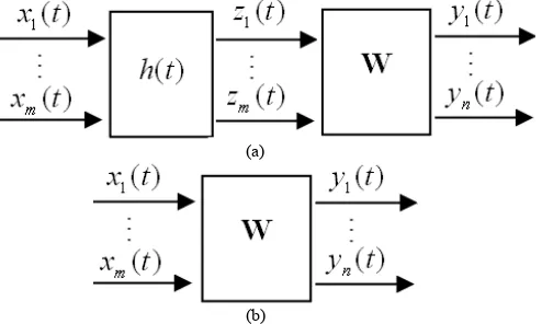
SDICA can be performed by the structure in figure.2. (a). As the first step, we apply a filter h t( ) to filter out the dependent subcomponents of the sources. Suppose
( )
h t exactly allows one independent subcomponent, say, the kth subcomponent si k, ( )t pass through. Let
( )
1,
( ) [ ( ), ,
k
k t = s t
s L . , ( )]T
n k
s t . Then the filtered
observations
( )
( ) ( ) [ ( ) ( )( )] k ( )
h t ∗x t =Ah t ∗ s t =As t . Therefore, in the second step, we just need to apply an ICA algorithm to the filtered observations, and we can obtain the demixing matrix W associated with the mixing matrix A.
(a)
(b)
Figure 2. (a) The structure to perform SDICA. (b) The linear instantaneous ICA demixing.
In the existing methods for SDICA, the frequency subband in which source sub-components are independent is determined by either some a priori information or exploiting the stronger assumption that at least two of the subcomponents are statistically independent. In practice, ICA is mainly used for BSS, so the exact a priori information on h t( ) is usually unavailable. The assumption that at least two of the subcomponents are statistically independent is not necessarily true, and the design of the optimal filter h t( ) for good performance remains a problem. It is therefore very useful to develop a method that adaptively estimates the optimal filter h t( ), such that the source-independent subcomponents pass through it and the dependent subcomponents are attenuated, and consequently both the mixing matrix A and the source-independent subcomponents can be recovered. Band-selective ICA (BS-ICA) is such a method [11].
stage. The parameters in the filter and the demixing matrix are adjusted by minimizing the mutual information between the outputs. By incorporating some penalty term, the prior knowledge on the independent subcomponents can be taken into account. The details can be found in [8].
Adjusting
W
[8]2 2
1
(
1)
( )
( )[
{ ( ), , ( )}
( ( ( )) ( ) )
{ [ ( ( )) ( ) )]}] ( ),
N T
T
k
k
k
diag E y
E y
E
k
k
diag E
k
k
k
η
ϕ
ϕ
+ −
=
−
+
−
y y
W
W
I
y
y
y
y
W
L
(3.3)
where
1 1
( )
y( ), ,
y
yN(
y
N)
Ty
y
ϕ
= ⎣
⎡
ϕ
L
ϕ
⎤
⎦
are theso-called score functions.,
diag E y
{ ( ), , (
12L
E y
N2)}
denotes the diagonal matrix withE y
( ), , (
12L
E y
2N)
as its diagonal entries, anddiag E
{ [ ( ) )]}
ϕ
yy y
T denotes the diagonal matrix whose diagonal entries are those on the diagonal ofE
[ ( ) )]
ϕ
yy y
T .Adjusting
h t
( )
[8]1
( )
( )
( )
{ ( )
(
)}
{
( )
(
)}
{
( )
(
)}
N
i i
k k k
T t
T t
T t
H y
I
H
h
h
h
E
t
t k
E
t
t k
E
t
t k
ϕ
ψ
β
=
∂
∂
=
−
∂
∂
∂
∂
= −
⋅
⋅
−
+
⋅
⋅
−
=
⋅
⋅
−
∑
y y y
y
y
W x
W x
W x
(3.4)
where
β
yT( )
t
=
ϕ
y( )
y
−
ψ
y( )
y
is defined as the score function difference (SFD). The SFD is an independence criterion; it vanishes if and only ify
i are mutually independent. Now the elements ofh t
( )
can be adjusted with the gradient-descent method.Eq.(3.3) and eq.(3.4) are the learning rules of BS-ICA. When the instantaneous stage and the filter stage both converge, the matrix
W
is the demixing matrix associated with the mixing matrixA
. The original sources can be estimated asWx
. Moreover, the outputsi
y
form the estimate of a filtered version of the independent subcomponentss
i I, .B Sparsity Based Multiresolution ICA Method
As the basic BSS model, assumptions can be made about the nature of the sources. Such assumptions form the basis for most source separation algorithms and include statistical properties such as independence and stationarity. One increasingly popular and powerful assumption is that the sources have a parsimonious representation in a given basis. These methods have come to be known as sparse methods. A signal is said to be sparse when it is zero or nearly zero more than might be expected from its variance. Such a signal has a probability density function or distribution of values with
a sharp peak at zero and fat tails. This shape can be contrasted with a Gaussian distribution, which would have a smaller peak and tails that taper quite rapidly. A standard sparse distribution is the Laplacian distribution, which has led to the sparseness assumption being sometimes referred to as a Laplacian prior. The advantage of a sparse signal representation is that the probability of two or more sources being simultaneously active is low. Thus, sparse representations lend themselves to good separability because most of the energy in a basis coefficient at any time instant belongs to a single source. This statistical property of the sources results in a nicely defined structure being imposed by the mixing process on the resultant mixtures, which can be exploited to make estimating the mixing process much easier. Additionally, sparsity can be used in many instances to perform source separation in the case when there are more sources than sensors. A sparse representation of an acoustic signal can often be achieved by a transformation into a Fourier, Gabor or Wavelet basis[26].
Sparse sources can be separated by each one of several techniques, for example, by approaches based on the maximum likelihood (ML) considerations[27], or by approaches based on geometric considerations[28]. In the former case, the algorithm estimates the unmixing matrix
1 −
=
W A , while in the later case the output is the estimated mixing matrix [29]. Here, we only consider the former case.
Now, we discuss the ML and the quasi1 ML solution of the BSS problem, based on the data in the domain of decomposition coefficients.
Let
D
be the new coefficient matrix of dimensionN T
×
, or called features, whereT
is the number of data points, and the coefficientsd
i form the columns ofD
. Note that, in general, the rows ofD
can be formed from either the samples of mixtures, or from their decomposition coefficients. In the latter case,{ :
ii
}
=
∈Ω
D
d
, whereΩ
are the subsets indexed on the transformation. We are interested in the maximum likelihood estimate ofA
given the data D.It is assumed that that the coefficients of the source signals
c
ik are i.i.d. random variables with the joint probability density function (pdf),
( )
( )
ik i kp
C
=
∏
p c
where
p c
( )
ik is of an exponential type:( )
ik qexp{ ( , )}
ikp c
=
N
−
v c q
.where
N
q is the normalization constant which will be omitted in the further calculations, since it has no effect on the maximization of the log-likelihood function. In a particular case wherein
|
|
( , )
q ik ik
c
v c q
q
=
(3.5)and
q
<
1
, the above distribution is widely used for modeling sparsity. Forq
=
1/ 2
it approximates rather well the empirical distributions of wavelet coefficients of natural signals and images[30]. A smaller q corresponds to a distribution with greater super-Gaussian that is more sparsity.Let
W
º
A
-1 be the unmixing matrix to be estimated. Taking into account that= +
D AC N,
If we neglect the effect of the noise, we arrive at the standard expression of the ICA log-likelihood, but with respect to the decomposition coefficients:
(
)
1 1
( , ) log ( )
log | det( ) |
[
] ,
M K
ik i k
L
p
K
v
q
= =
=
=
−
∑∑
D W
D
W
WD
.(3.6)In the case wherein (3.5), the second term in the above log-likelihood function (3.6) is not convex for
q
<
1
, and non-differentiable, therefore it is difficult to optimize. Furthermore, the parameter q of the true pdf is usually unknown in practice, and estimation of this parameter along with the estimation of the unmixing matrix is a difficult optimization problem. Therefore, it is convenient to replace the actualv
( )
with its hypothetical substitute, a smooth, convex approximation of the absolute value function, for examplev c
%
( )
ik=
c
ik2+
z
, withz
being a smoothing parameter. This approximation has a minor effect on the separation performance, as indicated by our numerical results. The corresponding quasi log-likelihood function is(
)
1 1
( ,
)
log | det( ) |
M K[
]
ik i kL
K
v
= =
=
−
∑∑
D W
W
WD
%
%
.(3.7) Maximization of
L
%
( ,
D W
)
with respect toW
can be solved efficiently by several methods, for example, the Natural Gradient (NG) algorithm [31] or, equivalently, by the Relative Gradient [32], as implemented in the BSS Matlab toolbox [33].The derivative of the quasi log-likelihood function with respect to the matrix parameter
W
is:(
)
1( , ( ))
[
( ( )) ( ) ]
( )
.
( )
T T
L
k
K
k
k
k
k
ϕ
−
∂
=
−
∂
D W
I
c
c
W
W
%
(3.8)
where
c
is the ’column stack’ version of C, and[
1]
( )
( ), , (
c
c
NK)
Tϕ
c
=
ϕ
L
ϕ
,where
( )
log
( )
( )
( )
ik ik
ik ik ik ik
ik ik ik
p c
d
c
p c
dc
p c
ϕ
= −
= −
′
arethe so-called score functions. Note, that, in this case,
( )
( )
ikc
ikv c
ikϕ
=
%
′
. The learning rule of the NaturalGradient algorithm is given by
(
)
( ,
( ))
(
1)
( )
( )
( )
( )
( )[
( ( )) ( ) ] ( ),
TT
L
k
k
k
k
k
k
k K
k
k
k
η
ϕ
∂
+ −
=
∂
=
−
D W
W
W
W
W
W
I
c
c
W
%
(3.9) where
η
( ) 0
k
>
is the learning rate. It has been proven that the natural gradient greatly improves learning efficiently in ICA than gradient method. In the original Natural Gradient algorithm, the above update equation is expressed in terms of the non-linearity, which has the form of the cumulative density function (cdf) of the hypothetical source distribution.In order to adapt the algorithm to purposes, we use hypothetical density with
v c
%
( )
ik=
c
ik2+
z
and thecorresponding score function is [29]
2
( )
ik ikik
c
c
c
ϕ
ζ
=
+
.The estimated unmixing matrix
W
ˆ
=
A
ˆ
-1 can be obtained by the quasi-ML approach, implemented along with the Natural Gradient, or by other algorithms, which are applied to either the complete data set, or to some subsets of data. In any case, this matrix and, therefore, the sources, can be estimated only up to a column permutation and a scaling factor. The sources are recovered in their original domain byˆ ˆ
( )t = ( )t = ( )t
y Wx WAs .
The next question is how to choose the proper transformation to dispose the mixtures. In this paper, Wavelet Packet (WP) transform is used to reveal the structure of signals, wherein several subsets of the WP coefficients have significantly better sparsity and separability than others.
In particular case of WP, we express each source signal and noise in terms of its decomposition coefficients:
( )
( )
j j
ki kil jl l
s t
=
∑
c
ϕ
t
(3.10)( )
( )
j j
ki kil jl l
n t
=
∑
e
ϕ
t
(3.11)where
j
represents scale level,k
represents sub-band index,i
represents source index andl
represents shift index.ϕ
jl( )
t
is the chosen wavelet also called atom or element of the representation space andc
kilj are decomposition coefficients. In our implementation of the described SDICA algorithm, we have used 1D WP for separation the mixed signals. If we choose the same representation space as for the source signals, we express each component of the observed datax
as( )
( )
j j
ki kil jl l
where
i
represents sensor index.Let vectors
d
l,c
l ande
l be the constructed from thel
th coefficients of the mixtures, sources and noises, respectively. From (2.1) and (3.12) using the orthogonality property of the functionsϕ
jl( )
t
we obtainl = l+ l
d Ac n , (3.13) Thus, when the noise is present Eq. (15) becomes
l l
d Ac . (3.14) Note, that the relation between decomposition coefficients of the mixtures and the sources is exactly the same relation as in the original domain of signals. Then, estimation of the mixing matrix and of sources is performed using the decomposition coefficients of the mixtures dl instead of the mixtures
x
.From (2.1) and (3.14) we see the same relation between signals in the original domain and WP representation domain. Inserting (3.14) into (3.12) and using (3.11) we obtain:
( ) ( )
j j
k t = k t
x As (3.15) as it was announced by (3.8) where no assumption of multiscale decomposition has been made. For each component
x
i of the observed data vectorx
, the WP transform creates a tree with the nodes that correspond to the sub-bands of the appropriate scale.As noted, the choice of a particular wavelet basis and of the sparsest subset of coefficients is very important with block signals. In particular, in the case of the WP representation, the best basis is chosen from the library of bases, and is used for decomposition, providing a complete set of features (coefficients).
In contrast, in the context of the signal source separation problem, it is useful to extract first an overcomplete set of features. Generally, in order to construct an overcomplete set of features, the approach to the BSS allows to combine multiple representations (for example, WP with various generating functions and various families of wavelets, along with DFT, DCT, etc.). After this overcomplete set is constructed, the ’best’ subsets (with respect to some separation criteria) is chosen and form a new set used for separation. This set can be either complete or undercomplete. [29]
Alternatively, the following iterative approach can be used. First, one can apply the Wavelet Transform to original data, and apply a standard separation technique to these data in the transform domain. As such separation technique, one can use the NG approach, or simply apply some optimization algorithm to minimize the corresponding log-likelihood function. This provides us with an initial estimate of the unmixing matrix
W
and with the estimated source signals. Then, at each iteration of the algorithm, we apply a multinode representation (for example, WP, or trigonometric library of functions) to the estimated sources, and calculate a measure of sparsity for each subset of coefficients. For example, one can consider thel
1 norm of the coefficients,
|
ik|
i k
c
∑
, itsmodification
∑
i k,log |
c
ik|
, or some other entropy-related measures. Finally, one can combine a new data set from the subsets with the highest sparsity (in particular, we can take for example, the best 10% of coefficients), and apply some separation algorithm to the new data. The iteration of the algorithm is completed. This process can be repeated till convergence is achieved.[29]When signals have a complex nature, the approach proposed above may not be as robust as desired, and the error-related statistical quantities must be estimated. [29] use the following approach. Firstly, applying the Wavelet Transform to original data, and apply a standard separation technique (Natural Gradient, clustering, or optimization algorithm to minimize the log-likelihood function) to these data in the transform domain. Secondy, given the initial estimate of
W
and the subsets of data (coefficients of mixtures) for each node, estimating the corresponding error variance, as described in[29]. Finally, one can choose a few best nodes (or, simply, the best one) with small estimated errors, combine their coefficients into one data set, and apply a separation algorithm to these data.IV. CONCLUSIONS
In this article, we considered the problem of Multiresolution subband blind source separation 你 (MRSBSS). We reviewed the feasibility of adaptively separating mixtures generated by the MRSBSS model and classified them into different categories, and identified new trends. After the perspective of MRSBSS is briefly presented, the general and detailed definition of the MSBSS model is given, the relationships among BSS, ICA and MRSBSS method is discuss simultaneously. Based on the minimization of the mutual information between outputs, we presented an adaptive algorithm for MRSBSS, which is called band-selective ICA. Then, taking the advantage of the properties of multiresolution transforms, such as wavelet packets, to decompose signals into sets of local features with various degrees of sparsity by the traditional NG method. Some simulations of these algorithms have been given to illustrate the performance of the proposed methods.
ACKNOWLEDGMENT
This work is partially supported by National Natural Science Foundation of China(Grant No.60672049) and the Science Foundation of Henan University of Technology(Grant No.08XJC027)
REFERENCES
[1] A. Hyvarinen, J. Karhunen, E. Oja, Independent
component analysis, John Wiley &Sons, New York, 2001.
[2] A. Cichocki, S. Amari, Adaptive Blind Signal and Image
Processing: Learning Algorithms and Applications, John Wiley&Sons, New York, 2002.
[3] J.F. Cardoso, “Multidimensional independent component
Acoustics, Speech, and Signal Processing (ICASSP’98), pp:1941-1944, Seattle, WA, USA, IEEE, 1998.
[4] A. Hyvarinen, P. Hoyer, “Emergence of phase and shift
invariant features by decomposition of natural images into independent feature subspaces”, Neural Computation, vol.12, no.7, pp.1705-1720, 2000.
[5] M. Kawanabe, K.R. Muller, “Estimating functions for
blind separation when sources have variance dependencies”, Journal of Machine Learning Research, vol.6, pp. 453-482 , 2005.
[6] A. Hyvarinen, P.O. Hoyer, M. Inki, “Topographic
Independent Component Analysis”, Neural Computation, vol.13, no.7, pp.1527-1558, 2001.
[7] F.R. Bach, M.I. Jordan, “Kernel Independent Component
Analysis”, Journal of Machine Learning Research, vol.3, pp.1-48, 2002.
[8] K. Zhang, L.W. Chan, “An Adaptive Method for Subband
Decomposition ICA”, Neural Computation, vol.18, no.1, pp.191-223, 2006.
[9] F.S. Wang, H.W. Li, R. Li, “Novel NonGaussianity
Measure Based BSS Algorithm for Dependent Signals”, Lecture Notes in Computer Science, vol.4505, pp.837-844, 2007.
[10]C.F. Caiafa, E. Salerno, A.N. Protoa, L. Fiumi, “Blind
spectral unmixing by local maximization of non-Gaussianity”, Signal Processing, vol.88, no.1, pp.50-68, 2008.
[11]M.R. Aghabozorgi, A.M. Doost-Hoseini, “Blind separation
of jointly stationary correlated sources”, Signal Processing, vol.84, no.2, pp.317-325, 2004.
[12]F. Abrard, Y. Deville, “A time-frequency blind signal
separation method applicable to underdetermined mixtures of dependent sources”, Signal Processing, vol.85, no.7, pp.1389-1403, 2005.
[13]R. Li, F.S. Wang, “Efficient Wavelet Based Blind Source
Separation Algorithm for Dependent Sources”, Advances in Soft Computing, Springer Press, vol.40, pp.431-441, 2007.
[14]P. Comon, “Independent component analysis, a new
concept?” Signal Processing, vol.36, no.3, pp.287-314, 1994.
[15]M. Zibulevsky, B.A. Pearlmutter, “Blind source separation by sparse decomposition in a signal dictionary”, Neural Computation, vol. 13(4), pp.863-882, 2001.
[16]M. Zibulevsky, Y.Y. Zeevi, “Extraction of a source from
multichannel data using sparse decomposition,” Neurocomputing, vol.49, pp.163-173,2002.
[17]F.M. Naini, G.H. Mohimani, M. Babaie-Zadeh, C. Jutten,
“Estimating the mixing matrix in Sparse Component Analysis (SCA) based on partial k-dimensional subspace clustering”, Neurocomputing, vol.71, no.10-12, pp.2330-2343, 2008.
[18]P. Bofill and M. Zibulevsky, “Underdetermined blind
source separation using sparse representation”, Signal Processing, vol.81, no.11, pp.2353-2362, 2001.
[19]S. Mallat, A Wavelet Tour of Signal Processing, Academic Press, New York, 1999.
[20]M.V. Wickerhauser, Adapted Wavelet Analysis from
Theory to Software, A.K. Peters, 1994.
[21]T.Tanaka, A. Cichocki. “Subband decomposition
independent component analysis and new performance criteria”. In Proc. IEEE Int. Conf. on Acoustics, Speech and Signal Processing (ICASSP’04), vol.5, pp.541–544, 2004.
[22]A. Cichocki, P. Georgiev. “Blind source separation
algorithms with matrix constraints”. IEICE Transactions on Information and Systems, Special Session on
Independent Component Analysis and Blind Source Separation, vol.E86-A , no.1, pp.522-531, 2003.
[23]A. Cichocki, T.M. Rutkowski, K. Siwek, “Blind signal
extraction of signals with specified frequency band”. In Neural Networks for Signal Processing XII: Proceedings of the 2002 IEEE Signal Processing Society Workshop. Piscataway, NJ: IEEE. pp.515-524, 2002.
[24]A. Hyvarinen. “Independent component analysis for
time-dependent stochastic processes”. In Proc. Int. Conf. on Artificial Neural Networks (ICANN’98) Skovde, Sweden, pp.541-546, 1998.
[25]O. Yilmaz, S. Rickard, “Blind separation of speech
mixtures via timefrequency masking”. IEEE Transactions on Signal Processing, vol.52, pp.1830-1847, 2004.
[26]P.D. O’Grady, B.A. Pearlmutter, S.T. Rickard, “Survey of
Sparse and Non-Sparse Methods in Source Separation ”, International Journal of Imaging System Technology, vol.15, no.1, pp.18-33, 2005.
[27]J.-F. Cardoso. Infomax and maximum likelihood for blind
separation. IEEE Signal Processing Letters, vol.4, no.4, pp.112-114, 1997.
[28]A. Prieto, C. G. Puntonet, and B. Prieto. A neural
algorithm for blind separation of sources based on geometric prperties. Signal Processing, vol.64, no.3, pp.315-331, 1998.
[29]P. Kisilev, M. Zibulevsky, Yehoshua Y. Zeevi, “A
Multiscale Framework For Blind Separation of Linearly Mixed Signals”, Journal of Machine Learning Research, vol.4, pp.1339-1364, 2003.
[30]R.W. Buccigrossi and E. P Simoncelli. Image compression
via joint statistical characterization in the wavelet domain. IEEE Transactions on Image Processing, vol.8, no.12, pp.1688-1701, 1999.
[31]S. Amari, “Natural gradient works efficiently in learning”, Neural Computation, vol.10, no.2, pp. 251-276, 1998.
[32]J.F. Cardoso, B. Laheld, “Equivariant adaptive source
separation”, IEEE Trans. Signal Processing, vol.44, no.12, pp.3017-3030, 1996.
[33]A. Cichocki, S. Amari, K. Siwek, T. Tanaka, ICALAB for
signal processing; Toolbox for ICA, BSS and BSE.
Available from http://www.bsp.brain.riken.jp/ICALAB/ICALABSignalPro
c/, 2004.
[34]Fasong Wang, Hongwei Li and Rui Li, “Efficient Blind
Source Separation Method for Harmonic Signals Retrieval”, Accepted for publication.
Hongwei LI was born in Hunan, China, in 1965. He received his Dr. degree in Applied Mathematics in 1996 from Beijing University. Currently, he is a professor in China University of Geosciences, China. His research interests include statistical signal processing, nonstationary signal processing, blind signal processing.
Rui LI was born in Henan, China, in 1979. She received her M.S. degree in Computation Mathematics in 2008 from Zhengzhou University. Currently, she is a lecture in Henan University of Technology. Her research interests include blind signal processing, intelligence optimization.