Dynamic Modeling of Biotechnical Process Based on Online Support Vector Machine

Dynamic Modeling of Biotechnical Process

Based on Online Support Vector Machine

Xianfang Wang1, 2

1. Jiangnan University / School of Communication and Control Engineering, Wuxi, China 2. Henan Institute of Science and Technology / Department of Information Engineering, Xinxiang, China

Email: [email protected]

Zhiyong Du

Henan Mechanical and Electrical Engineering College/ Department of Computer, Xinxiang, China Email: [email protected]

Jindong Chen and Feng Pan

Jiangnan University / School of Communication and Control Engineering, Wuxi, China Email: [email protected]

Abstract—Due to the complexity and high non-linearity of biotechnical process, most simple mathematical models cannot describe the behavior of biochemistry systems very well. Therefore, dynamic modeling of biotechnical process is indispensable. Support vector machine (SVM) is a novel machine learning method, which is powerful for the problem characterized by small sample, non-linearity, high dimension and local minima, and has high generalization. But currently most support vector machine regression (SVR) training algorithms are offline, which could not be suit for time-variant system. So an improved SVM called online support vector machine was presented to modeling for the dynamic feature of fermentation process. The model based on the modified SVM was developed and demonstrated using simulation experiments. Some models based on SVM were also presented. The result shows that the modeling based online SVM is superior to modeling based on SVW. Index Terms—dynamic modeling, biotechnical process, online support vector machine, on-line estimation

I. INTRODUCTION

Biotechnical process is a kind of complicated reaction processes. Control of biotechnical process that was in nearly empty for twenty years has recently gained an unprecedented development because the methods of system identification and optimized control tend to mature. An accurate and effective mathematical model is a must for implementing control and optimization of biotechnical processes.

Three kinds of model are generally used for describing the characteristics of biotechnical processes and for the purpose of process control and optimization: the white-box, the black-box model, the gray-box. The white-box is one kind of unstructured dynamic model, for example, the Monod growth model and the Luedeking-Piret product formation model, uses ordinary differential equations to describe the time changes of those state

variables such as the concentrations of cells, substrates, metabolic products, etc. The unstructured model is mainly used for the purposes of off-line process prediction, control, and optimization. There are two major disadvantages generally accompany with the unstructured model [1], one is that heavy works are required to identify a large amount of model parameters while the physiological meanings of those parameters is not so clear; the other is that the un- structured model can not really grasp the dynamic changes due to the changes of environmental factors, operating conditions, and the fermentation batch runs, therefore, the general predicting and control performance based on the model is limited. The black-box model is completely based on the input– output series data or the apparent behaviors of the processes, and the real mechanisms or natures of the metabolic reactions are not considered at all. The model parameters are not of any physical or chemical meanings. The artificial neural network (ANN) model is one kind of black-box model, which is quite popular in fermentation process modeling for its excellent ability dealing with the complex and non-linear process characteristics. However, a fetal shortcoming of the ANN model is that, a huge amount of experimental data pairs must be provided for training the ANN model, otherwise the general performance of the model will be significantly deteriorated [2, 3]. The gray-box is one kind of hybrid-model, such as, fuzzy logic inference model is a human experience and knowledge-based qualitative model, its general prediction power and accuracy largely rely on the experiential fuzzy logic rules and membership functions, whereas the development and adaptive adjustment of fuzzy logic rules and membership functions are a time and labor consuming process [4].

of on-line measurement based on hardware sensors [6, 7], they have their own limitations, and the corresponding on-line instruments are expensive and difficult in maintenance.

Support vector machine (SVM) is a new and valid machine-learning algorithm and has been well used for classification, function regression, and time series prediction, etc. [8-11]. Compared with neural network, SVM has good generalization ability, and is especially suitable for machine learning in small sample condition. The training algorithm of SVM will not run into local minimum point. Also it can automatically construct the structure of system model. However, currently most support vector machine regression (SVR) training algorithms are offline, but online SVR algorithm is more useful when the system to be identified is time-variant, because this kind of algorithms can automatically track changes of system model with varying and time-lagging characteristics [12, 13].

According to the shortcoming in above generally modeling method in biotechnical processes, a dynamic modeling was built by utilizing the mechanism of fermentation and characteristics of online SVM in this paper. This method was adopted for glutamic acid fermentation process, the result shows that the dynamic modeling based on the online-SVR algorithm can get a good result.

The paper is organized as follows: In Section Ċ the improved online SVR algorithm is introduced in detail. In Section ċ, two modeling method of glutamic acid concentration are designed based on SVM and online SVM respectively. Two simulation results are given to show the validity of two modeling methods. In Section Č, the comparisons of online SVR algorithm-based modeling with offline SVR algorithm for modeling biotechnical process. Some conclusions are obtained and put forward in Sectionč.

II. ONLINESUPPORT VECTOR REGRESSION

A. Support Verctor Machine

SVM is an excellent method aiming to finite data points based on statistical learning theory (SLT) [14, 15], advanced by Vapnik in 1990’s. Given a training sample set:

T

{ ,

x y i

i i

,

1, 2,

l

}

,

N i

x R and

y

_i



R

,

1

( ) ( )

l i i i

f x

_¦

wI x b (1) where { ( )} 1

l i x i

I is the data in features space, { ( )} 1 l i i

w x and b are coefficients. They can be estimated by minimizing the regularized risk function

2 1 1 1 ( ) ( , ( )) 2 l i i

R C C L y f x w

l

¦

H (2)

where L y f x_H( , ( ))_i is the so-called loss function measuring the approximate errors between expected output yi and calculated output f x( )i and C is

regularization constant determining the trade-off between the training error and the generalization performance. The

second term,1 2

2 w , is used as a measurement of function

flatness. Introduction of slack variables ,[ [ _{leads (2) to}

the following constrained function

¦

l i i i b

w J w C

1

* 2

,

, ₂ ( )

1

min [ [

[ (3) s.t. * * ( ) ( )

1, 2 , ... 0

0

i i i

i i i

i

i

y w x b

w x b y

i l

I H [

I H [

[ [

d

­

° _d

° ® t ° ° t ¯

Using the duality principle, the equation (3) could be changed equation (4)

*

* *

, _{, 1}

* *

1 1

1

max{ ( )( )

2

( ) ( )}

l

D i i j j i j

i j

l l

i i i i i

i i

L x x

y

D D D D D D

H D D D D

˜

¦

¦

¦

˄4˅

s.t.

*

1

( ) 0

0 0 l i i i i j C C D D D D ­

° _{d d}

®

° _{d d}

¯

¦

Although non-linear function I is usually unknown all computations related to I can be reduced to the form

( )xT ( )y

I I , which can be replaced with a so-called kernel function K(xi,xj) I(xi)˜I(xj) that satisfies

Mercer’s condition [16, 17]. Then, Eq. (1) becomes the explicit form

* *

( , ) ( ) ( , )

i

i i i i i

x S V

f x D D D D K x x b



¦

ˈ (5)

In equation (5), Lagrange multipliers Diand * i D satisfy the equalityD Di i 0,Di 0,Di 0,i 1, ,l

u t t . Those

vectors with Di z0 are called support vectors, which contribute to the final solution.

B. Online Support Verctor Machine

The Online Support Vector Regression algorithm main purpose is to verify these conditions after that a new sample is added. The online SVR algorithm can be described as follows:

LetTi Di Di,

use equation (6), define a margin function h(xi) as,

1

( ) ( ( , )

l

i i i i i i

j

h x f x˅y

_¦

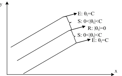
TK x x b y (6)

R: |și|=0

E: și=C

E: și=C

S: 0<|și|<C

S: 0<|și|<C

Figure 1.Three subsets gotten from training samples set

Set E: Error support vectors,

) { i , ( i }

E i T C h x t H , Set S: Margin support vectors,

)

{ | | 0 i , ( i }

S i T C h x H , Set R: Remaining samples,

)

{ i 0 , ( i }

R i T h x d H

When a new sample xcis added, the goal is to let xc

enter one of the three sets, while KKT condition still can be satisfied automatically.

At first, let T_c 0, from equation (6), we can obtain:

1

( ) ( ( , )

l

c c c j c j c

j

h x f x˅y

_¦

T K x x b y (7)

then we gradually change the value of

T

_c and at the same time make all other samples satisfy KKT condition. The change of

T

_c may change the values of

T

_i and h(xi) of

other samples. It satisfies the formula:

1

( ) ( , ) ( , )

l

i i c c i j

j

h x K x x T K x x b

' '

¦

' (8)

1

0

l

c i

i

T

¦

T (9)

the relation among 'T_c,'T_iand b could be obtained:

1 l s s c s b T E T T ' ª º «_' » « _{» '} « » « » ' « » ¬ ¼ (10) where i s S

T  , lsis sample number of set S, and

1 1

1 ( , ) =

( , )

ls ls

s s c

s s c

K x x R

K x x

E E E E ª º ª º « » « » « » « » « » « » « » « » « » «_¬ »_¼ ¬ ¼ (11) where

1 1 1

1

0 1 1

1 ( , ) ( , )

1 ( , ) ( , )

ls

ls ls ls

s s s s

s s s s

K x x K x x R

K x x K x x

ª º « » « » « » « » « » ¬ ¼ (12)

The relation among'Tcand 'h x( )i can be obtained

equation (13): 1 2 ( ) ( ) ( ) ln n n c n h x h x h x J T ' ª º « » ' « » _' « » « » «' » ¬ ¼ (13) where i n

x  ‰ ‰E R C,ln is the sample number of set

E‰ ‰R CR, and

1 1 1

1

2 2 1 2

1

1 ( , ) ( , )

( , )

( , ) 1 ( , ) ( , )

=

( , ) 1 ( , ) ( , )

ls

ls

ln ln ln ls

n s n s

n c

n c n s n s

n c n s n s

K x x K x x K x x

K x x K x x K x x

K x x K x x K x x

J E ª º ª º « » « » « » « » « » « » « » « » « » « » ¬ ¼ ¬ ¼ (14) Matrix R can be updated with a recursive algorithm according to following formula when a new sample xi is

added to set S:

0 1

1

0 1

0 0 0

T

i

R

R E E

J ª º « » _{ª º} « » _{ª º} « » ¬ ¼ « » _{¬ ¼} « » ¬ ¼ (15) where 1 ( , ) = R ( , ) ls i ls i s s s s

K x x

K x x

E ª º « » « » _{« »} « » « » ¬ ¼ (16) 1

( , ) 1 ( , ) ( , )

ls

i K x xi i K xs xi K xs xi

J _¬ª º_¼ (17)

when a sample xi is removed from R, matrix R is updated

as

, ,

, ,

, i k k j i j i j

k k

R R R R

R

(18)

where i j, [1,, ,k k2,,s_ls1].

From above, online SVM regression training algorithm is consisted of two sub-algorithms: incremental algorithm and decremental algorithm.

The main idea of incremental algorithm is that: when a sample xc is added to training sample set, we gradually change its Tc and h(xc) until xc enter into of one of three

sets, and during the process some other samples are also updated from one of sets S, R, and E to another because they are influenced by the change of sample xc. The goal

of the incremental algorithm is to make all samples satisfy the KKT condition while a new sample is added to training sample set.

The main idea of decremental algorithm is that: a sample with zero value of Tc can be removed safely since

it has no influence to SVM model; when a sample xc is to be removed from training sample set, we gradually change its Tc and h(xc) until Tc change to zero, and

influenced by the change of sample xc. The goal of the decremental algorithm is to make all samples satisfy the KKT condition while a useless sample is removed out of training sample set.

After long math proofs and analysis the algorithm is finally shown. It’s in a pseudocode format. The input requested from an Online Support Vector Regression is the following:

INPUTS

1. Training Set {xi,yi, i = 1…l} 2. Wheights Ti, i = 1…l

3. Bias b

4. Training Set partition into Supposed(S), Error Set (E) and Remaining Set(R)

5. Params:H, C, Kernel Type and Kernel Params 6. R Matrix

7. New Sample c= (xc, yc)

OUTPUTS

1. New Training Set {xi,yi, i = 1…l + 1} 2. New CoefficientsTi,i= 1…l + 1

3. New Bias b

4. New Training Set partition 5. New R Matrix

NEW TRAINING ALGORITHM 1. Add (xc,yc) at the Training Set 2. SetTc 0

3. Compute f(xc) and h(xc) 4. If (|h(xc)| <H)

4.1Add New Sample to the Remaining Set and Exit 5. Compute h(xi), i = 1…l

6. While (New Sample is not added into a set) 6.1 Update the valuesE and J

6.2 Find Least Variations (Lc1, Lc2, Ls, Le, Lr) 6.3 Find Min Variation

c T

' = min (Lc1, Lc2, Ls, Le, Lr)

6.4 Let Flag the case number that determinates 'Tc

(Lc1 = 1, Lc2 = 2, Ls = 3, Le = 4, Lr = 5) 6.5 Let xl the sample that determines'Tc

6.6 Update 'Tc,'Ti,i= 1…l and b

6.7 Update h x( ),i i ‰E R

6.8 Switch Flag 6.8.1 (Flag = 1)

6.8.1.1 Add New Sample to Support Set 6.8.1.2 Add New Sample to R Matrix 6.8.1.3 Exit

6.8.2 (Flag = 2)

6.8.2.1 Add New Sample to Error Set 6.8.2.2 Exit

6.8.3 (Flag = 3) 6.8.3.1 If (_l = 0)

6.8.3.1.1 Move Sample l from Support to Remaining Set

6.8.3.1.2 Remove Sample l from R Matrix 6.8.3.2 Else[Tl |C|]

6.8.3.2.1 Move Sample l from Support to Error Set

6.8.3.2.2 Remove Sample l from R Matrix 6.8.4 (Flag = 4)

6.8.4.1 Move Sample l from Error to Support 6.8.4.2 Add Sample lto R Matrix

6.8.5 (Flag = 5)

6.8.5.1 Move Sample l from Remaining to Support Set

6.8.5.2 Add Sample l to R Matrix

At the beginning, Online SVR tries to check if the new sample can be inserted in the Remaining Set. This is the best case, because it is fast and does not increase the complexity of the machine. If this does not happen, it starts a cycle that finishes only when the new sample is added to Support or Error set (cases 1 and 2). At each iteration, a sample migrates from one set to another. Each migration passes through Support Set, so that at every iteration the R matrix (that is correlated to support samples) changes. Because this is a common and the most expensive operation, in the next sections it will be explained a method to efficiently update the R Matrix.

ċ. MODELING OF GLUTAMIC ACID

FERMENTATION PROCESS

A. Modeling of glutamic acid concentration

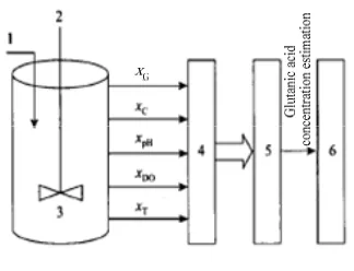
We are using a batch glutamic acid fermentation process, which consists of a fermentor and its peripherals: air compressor, agitation system, heat exchanger and control equipment for pH, temperature, dissolved oxygen and foam leave. The fermentor is 30 m3(Food Industry Institute, Tianjin, China) with pH, DO, and temperature optimal control. Above methods were applied in constructing the glutamic acid concentration soft-sensor model of the fed-batch fermentation for Glutathione production by Succharomyces cerevisiue. According to the mechanism of fermentation procedure, we select the temperaturex iT( ), pH valuexpH˄i), dissolved oxygen

concentration xDO( )i , CO2 partial pressure of exhaust gas

2( ) CO

x i , and glutamic acid concentrationx iG( ) as the

input variables of the glutamic acid concentration soft-sensor model because these parameters are related closely with the glutamic acid concentration, selectx iG( +1) as

Figure 2. Modeling of glutamic acid concentration 1-glucose; 2-agitation; 3-fermentor; 4-data process; 5- glutamic acid concentration soft-sensor; 6-control system

There are 10 batches of production data, each batch express a complete fermentative process. Every batch is divided into 15 samples. 7 batches data as training data and the other regard as test data.

B. Modeling based on SVM

For the reflection fermentative process’s misalignment relations, use the radial direction base nuclear function,

2

( , ) exp( ) 2

i j i j

x x K x x

V

, Therefore the SVM

parameter mainly has the insensitive coefficient İ, penalty coefficient C and the breadth factorV . Uses various sample points relative error's average value (the mean error ratio) the computation model training error and the prediction error. Using different penalty coefficient C, the insensitive coefficient İ and the breadth factor V , the computation training error and the prediction error as shown in Tableĉ.

TABLE I.

INFLUENCE OF PARAMETER ABOUT MODELING QUALITY

C H V Training MSE

100 0.5 0.6 0.2355

100 0.5 1 0.2354

100 0.5 10 0.2469

100 0.5 20 0.4575

100 0.5 25 1.8397

100 0.1 0.6 0.0096

100 0.9 0.6 0.7626

100 1.1 0.6 1.1391

100 1.5 0.6 2.1179

100 2.0 0.6 3.7649

50 0.5 0.6 0.2355

40 0.5 0.6 0.2378

30 0.5 0.6 46.5735

From Tableĉdata analysis, it can be found clearly that C is bigger, the penalty is stricter to the error, i.e. to fits the accuracy requirement to be high, causes the training

becomes difficult, very spends the time. Therefore along with C enlargement, the fitting error and the prediction error will reduce, when after C increases to the certain extent, the fitting error tends to be stable, when C is oversized, will present “the fitting” the phenomenon, this time the prediction error instead will increase.

İ is the reflection of the noise sensitive degree to the input variable, uses for to control the model fitting precision, İ is bigger, the fitting precision is lower, derives the support vector number are few, the model complex degree is low, its pan-ability is strong; Otherwise, İ is smaller, the fitting precision is high, supports the vector number to increase, the model order of complexity is high, its pan-ability is low.

When

V

is small, the model fitting performance is good, but too small will create the pan-ability variation; Otherwise,

V

is too big, supports the vector the influence to be excessively strong, the model achieves the enough precision with difficulty, easy to produce “owes the fitting”.

In order to judge the performance of the model, the mean square error (MSE) is selected. When the training MSE=0.0096, then parameter V =0.6ǃC =100ǃİ =0.1 are selected. The training result of Glutamic acid concentration based on SVM is shown in Fig.3.

Figure 3. Predicting result of modeling based on SVM

From Figure 3, we can see that the predicting result of generalization of this method is not ideal, so it need to be improved.

C. Modeling based on online SVM

In order to improve the precision and ability of generalization of the soft-sensor, the modified model based on the online SVM is developed. The same inputs and architecture of model are used as that in above section.

The TableĊ shows the parameters of the SVR used during the stabilization test.

TABLE II.

TRAINNING PARAMETERS OF THE STABLIZATION SET

Training İ C V

Default 0.01 3 50

Increasing C 0.01 10 50 Decreasing C 0.01 1 50

IncreasingH 0.1 3 50

DecreasingH 0.0001 3 50 Increasing Kernel Param 0.01 3 100 Decreasing Kernel Param 0.01 3 10

The C parameter influences Support and Error Set. From these results, it seems that it should be used with an increment of speed. When used in an application, it could be changed to avoid overfitting and underfitting. H is more critical than C because it influences all the samples. In fact, the number of iterations needed is higher and, sometimes the algorithm speed is lower than if we were to restart the training.

The detailed process of modeling is as following:

Step 1 Construct a new SVM training set

X{

2

{ , , , , )

i i i i i

i T pH co DO E

X x x x x x }have summarized l samples.

Step 2 Use incremental algorithm of online SVR algorithm to train system model.

Step 3 If number of training samples is out of threshold max_sp, use decremental algorithm to remove redundant samples.

Step 4 Compute predicting error e= x i_G( +1) -x i_G( ), if e is less than a threshold min_error, end training process, and go to step 5, else return to step 1.

Step 5 Using the model to predict the glutamic acid concentration x i_G( +1).

Step 6 Return to step 4.

Figure 4. Predicting results of modeling based on online SVM

IV. COMPARING OF RESULTS BETWEEN TWO METHODS

The new proposed modeling of biotechnical process is easy to use and has good real-time processing ability and adaptively which come from the adoption of online SVR algorithm. Here we compare online SVR algorithm-based system identication with offline SVR algorithm for modeling biotechnical process.

A.. Usability

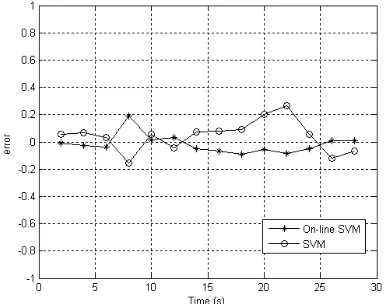
The Comparisons of predicting error between the two models are shown in Fig. 5

Fig. 5 shows that the modeling based on online SVM achieved more excellent capability of generalization than the one based on standard SVM. The performance index of the improved model is: MSE=0.0023. It shows a higher precision of approximation than modeling based on standard SVM.

From comparison of predicting errors, it is concluded that the improved model shows outstanding performance than the one built on the standard SVM because this modified algorithm possesses both advantages of sparseness and robustness.

Figure 5. Comparisons of predicting error between two models

Online and offline SVR algorithms are all easy to use. They have uniform structure of model, and only have several adjust able parameters. While the structure of NN must be selected, including the tier number of NN, inner node number of each tier, and initial values of weight coefficients. If bad parameters are selected, it will lead to a NN model with bad performance or very long training time. So SVR algorithms can be more easily used to construct system model than NN.

B. Speed

Speed of online SVR algorithms is faster than that offline one. The comparison of training time and testing time between modeling SVM and online SVM method is shown in TableĊ.

In MATLAB simulation experiments, training processes of online SVR algorithm as shown in TableĊ

take less than 2.9843 s.

written in c code, while our algorithm is written in MATLAB code).

TABLE III.

COMPARING OF THE TRAINING AND TESTING TIME

From Table ċ, it is clearly found that the training and the testing time of modeling based on online SVM are shorter than the SVM. We can see that Online SVR is quicker than SVM in training.

From above analyze, it is illuminated that the modeling based on online SVR for biotechnical process has very good performance.

C. .Adaptivity

Online SVR algorithm can automatically track variance of indented plant model, so it can be used to construct dymatic model of time-varying system. Offline SVR algorithm can not be used to construct model of time-varying system.

V. CONCLUSION

Modeling of biotechnical process has received much attention in recent years, and the requirement of the online predicting models is practical in real-world applications. This paper develops an online SVM model to predict the concentration of production, and it can provide promising prediction results.

In order to achieve the aim of on-line estimating the glutamic acid concentration, the method of SVM is introduced as the soft-sensor, and the SVM based model obtains a certain precision and generalization ability. Nevertheless, an improved SVM called online SVM is developed as the soft-sensor model for the fermentation process and better performance is achieved. Compared with the conventional SVM model, it can not only receive data in sequence and determine dynamically the optimal prediction model, but also can lead to high prediction performance; therefore, the applications of the online SVM method in biotechnical process is a good interesting attempt and it may be worthy to test its value in more areas. Additionally, the computational problem in the proposed approach with the numerical optimization in a high-dimensional space may suffer from the course of dimensionality. How to solve this problem will be our future research work.

ACKNOWLEDGMENT

This work is supported by the National High-tech Research and Development of China (863 project) (No.2006AA020301-11). Therefore, it is necessary for the stability conditions to be investigated in the multi-regions.

REFERENCES

[1] K. Shimizu, K. Furuya, Optimal operation derived by Green’s theorem for the cell-recycle filter fermentation focusing on the efficient use of the medium, Biotechnol. Prog. 10 (1994), pp. 258–262.

[2] J.F. Pollard, M.R. Broussard, D.B. Garrison, K.Y. San, Process identification using neural networks, Comput. Chem. Eng. 16 (4) (1992), pp. 253–270.

[3] L.H. Ungar, B.A. Powell, S.N. Kamens, Adaptive networks for fault diagnosis and process control, Comput. Chem. Eng. 14 (4/5) (1990), pp.561–572.

[4] M. Kishimoto, Application of fuzzy logic theory to bioprocesses and its problem, Biosci. Ind. (Jpn.) 49 (7) (1991) , pp.18–22.

[5] Olsson, L., Nielson, J., “Online monitoring of biomass in submerged cultivation”, Trends Biotechnol., 15(1l), ( 1997) , pp.5017-522.

[6] Wang, Y.J., Fan, Y., “Studies of on-line and in-situ measuring method for biomass concentration”, Prog. Biochem.Biophys., 27(4) (2000), pp:387-390. (in Chinese) [7] Wang, W., Yang, H.L., Lu. X.F., Yang, S.L., “The

application of ultrasonic in fermentation engineering”, J. Wuxi Univ. Light Ind., 21(3), (2002), pp.322-326. (in Chinese)

[8] P.M.L. Drezet, R.F. Harrison, Support vector machines for system identification, in: UKACC International Conference on CONTROLÿ98, UK, 1998, pp. 668̢692. [9] K.R. Mu¨ ller, A.J. Smola, Predicting time series with

support vector machines, in: Proceedings of ICANN’97, Lecture Notes in Computer Science, vol. 1327, Springer, Berlin, 1997. pp. 999–1004.

[10] A.J. Smola, B. Scho¨ lkopf, A tutorial on support vector regression, Neurocolt Technical Report, Royal Holloway College, University of London, 1998.

[11] J.A.K. Suykens, Nonlinear modeling and support vector machines, In: IEEE Instrumentation and Measurement Technology Conference, Budapest, Hungary, 2001, pp. 287–294.

[12] M. Martin, On-line support vector machines for function approximation,Technical Report LSI-02-11-R, Software Department, Universitat Politecnica de Catalunya, Spain, 2002.

[13] D.C. Wang, et al., Support vector machines regression on-line modeling and its application, Control Decision 18 (1) (2003), pp. 89–91,95.

[14] Vapnik, V.N., Statistical Learning Theory, Wiely, New York (1998).

[15] Vapnik, V.N., The Nature of Statistical Learning Theory,2nd Edition, Springer-Verlag, New York (1999). [16] V. Vapnik, The Nature of Statistical Learning Theory,

Springer, NewYork, 1995.

[17] V. Vapnik, Statistical Learning Theory, Wiley, New York, 1998.

[18] J.S.Ma,T.James,P.Simon,Accurateon-linesupportvector regression, NeuralComput.15(11)(2003), pp.2683-2704

Zhiyong Du, 1967.05, associate professor; Henan Mechanical and Electrical Engineering College, China, his research interests include machine learning, modeling and optimized controlling.

E-mail:[email protected]

Jindong Chen, 1983.10, doctoral student, Jiangnan University, China, his research fields include modeling and optimized controlling of biotechnical process process, etc.

E-mail: [email protected]