Error Analysis in Finite Volume CFD

(1)

Error Analysis in Finite Volume

CFD

Franjo Juretic

Thesis submitted for the

Degree of Doctor of Philosophy of the University of London

and

Diploma of Imperial College

Department of Mechanical Engineering

Imperial College London

(2)

Abstract

This study was aimed towards improving the accuracy of Computational Fluid Dy-namics (CFD) by developing methods for reliable estimation of the discretisation error and its reduction.

A new method for error estimation of the discretisation error for the second-order accurate Finite Volume Method is presented, called the Face Residual Error Estimator (FREE), which estimates the discretisation error on the cell faces. The es-timator is tested on a set of cases with analytical solutions, ranging from convection-dominated to diffusion-convection-dominated convection-dominated ones. Testing is also performed on a set of cases of engineering interest and on polygonal meshes.

In order to automatically produce a solution of pre-determined accuracy an au-tomatic error-controlled adaptive mesh refinement procedure is set up. It uses local mesh refinement to control the local error magnitude by refining hexahedral cells parallel to the face with large discretisation error. The procedure is tested on four cases with analytical solutions and on several laminar and turbulent flow cases of engineering interest. It was found able to produce accurate solutions with savings in computational resources.

In order to explore the possibilities of different mesh structures, a mesh generator producing polyhedral meshes based on the Delaunay technique is developed. An adaptive mesh generation technique for polyhedral meshes is also developed and is based on remeshing parts of the mesh which are selected for refinement. The mesh adaptation technique is tested on a case with an analytical solution. A comparison of accuracy achieved on quadrilateral, triangular and polygonal meshes is also given, where quadrilateral meshes perform best followed by polygonal meshes.

(3)

3

Acknowledgements

I would like to express my gratitude to my supervisor Prof A. D. Gosman for his interest and continuous guidance during this study.

I would like to use the opportunity to thank my colleagues from Prof Gosman’s CFD group, especially Dr. Hrvoje Jasak, Mr. Henry Weller and Mr Mattijs Janssens for developing the FOAM C++ simulation code which made the implementation of the ideas easier. Their support and suggestions were invaluable.

This study and the text of this thesis has benefited a lot from the numerous suggestions and comments by Dr. Hrvoje Jasak.

It would be unfair not to thank Mrs Nicky Scott-Knight and Mrs Susan Clegg for arranging administrative matters.

Finally, the financial support provided by the Computational Dynamics Ltd. is gratefully acknowledged.

(4)

(5)

List of Figures

3.1 Computational cell . . . 40

3.2 Mesh non-orthogonality . . . 42

3.3 Mesh skewness . . . 42

3.4 Variation of φ near the face . . . 49

3.5 Non-orthogonality treatment . . . 51 3.6 Boundary cell . . . 57 3.7 Square mesh . . . 59 3.8 Triangular mesh . . . 59 3.9 Hexagonal mesh . . . 59 3.10 Split-hexahedron mesh . . . 60

4.1 Inconsistency of the interpolated values on the face . . . 84

4.2 Distance between points on non-orthogonal mesh . . . 90

4.3 Solution domain and boundary conditions for the jet case . . . 92

4.4 Starting mesh for the jet case (10 x 4 cells) . . . 93

4.5 Velocity field for the jet case [m/s] (80 x 32 mesh) . . . 94

4.6 Pressure isobars for the jet case [m2_/s2_{] (80 x 32 mesh) . . . 94}

4.7 Velocity error field for the jet case [m/s] (80 x 32 mesh) . . . 95

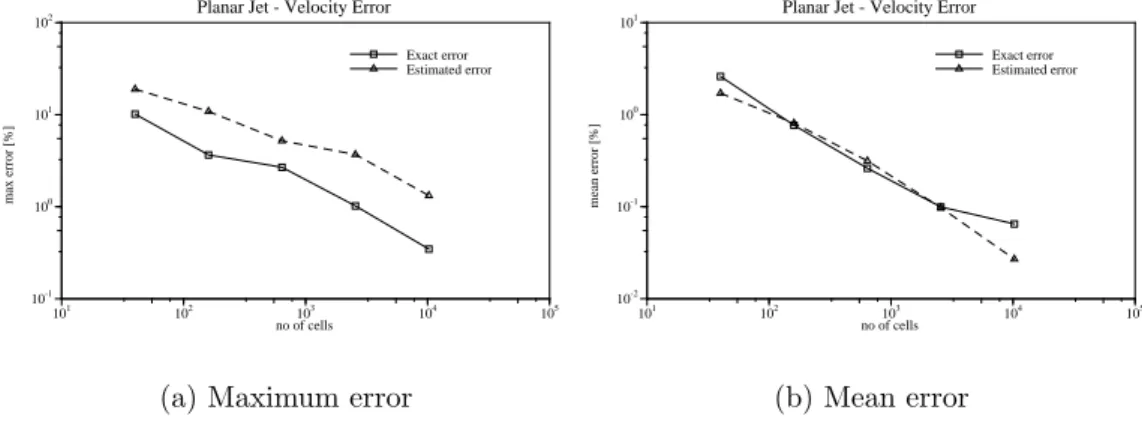
4.8 Variation of errors with uniform mesh refinement for the jet case (_|Unorm|= 2.474m/s) . . . 96

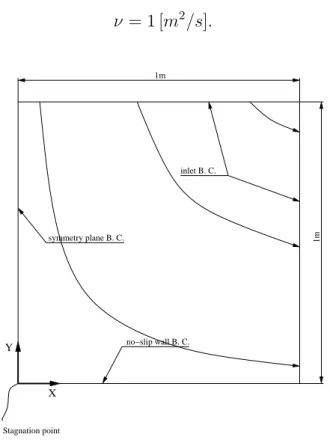
4.9 Solution domain and boundary conditions for the stagnation flow . . 97

4.10 Velocity and pressure for the stagnation flow (40 x 40 mesh) . . . 98

4.11 Velocity error fields for the stagnation flow [m/s] (40 x 40 mesh) . . 98

4.12 Variation of errors with uniform mesh refinement for the stagnation flow (_|Unorm|= 1.107m/s) . . . 99

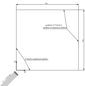
4.13 Solution domain and boundary conditions for the convection trans-port case . . . 100

(10)

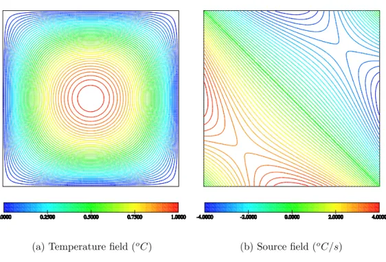
4.14 Temperature and source fields for the convection transport case (40

x 40 mesh) . . . 101

4.15 Error fields for the convection transport case [o_{C] (40 x 40 mesh) . . 101}

4.16 Uniform mesh . . . 102

4.17 Variation of errors with uniform mesh refinement for the convection transport case (Tnorm = 1oC) . . . 102

5.1 A split-hexahedron cell with left face split in one direction shared with two cells. The top face is cross-split and shared with four cells . 110 5.2 Directional splitting of cells . . . 111

5.3 Refinement of split-hexahedron cells . . . 111

5.4 Node distances at a split face . . . 112

5.5 Additional splitting of cells . . . 113

5.6 Consistency over a split face in 2D (dotted lines represent the selected refinement) . . . 114

5.7 Consistency over a cross-split face in 3D (dotted lines represent the selected refinement) . . . 115

5.8 Treatment of incompatible cell splitting directions in 3D (dotted lines represent the selected refinement) . . . 115

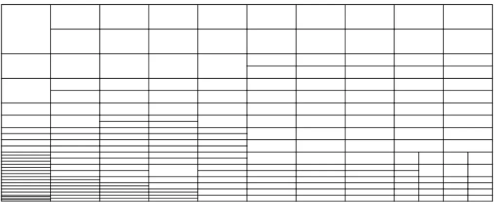
5.9 Mesh after 6 cycles of refinement for the jet case (209 cells) . . . 117

5.10 Variation of velocity errors with adaptive refinement for the jet case (_|Unorm|= 2.474m/s) . . . 117

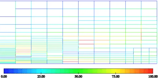
5.11 Velocity errors after 6 cycles of refinement for the jet case [m/s] (209 cells) . . . 118

5.12 Estimated errors on the faces of the final mesh with 209 cells (given as percentage of the maximum estimated error on that mesh) . . . 119

5.13 Meshes for the creeping stagnation flow . . . 121

5.14 Velocity errors after 4 cycles of refinement for the creeping stagnation flow [m/s] . . . 122

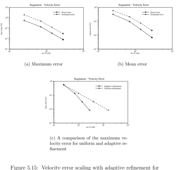
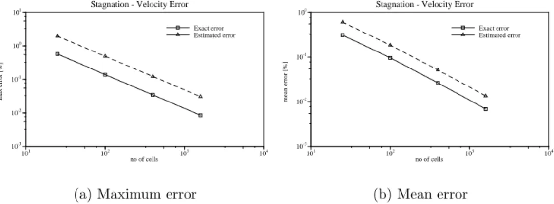
5.15 Velocity error scaling with adaptive refinement for the creeping stag-nation flow (_|Unorm|= 1.107m/s) . . . 123

5.16 Estimated errors on the faces of the final mesh with 280 cells (given as percentage of the maximum estimated error on that mesh) . . . 124

(11)

List of Figures 11 5.18 Variation of velocity errors with adaptive mesh refinement for the

stagnation flow (Second calculation) (_|Unorm|= 1.107m/s) . . . 126

5.19 Velocity error fields after 2 cycles of adaptive refinement for the stag-nation flow (Second calculation) [m/s] . . . 126 5.20 Mesh after 3 cycles of refinement for the convection transport case . . 127 5.21 Fields after 3 cycles of refinement . . . 128 5.22 Variation of temperature errors with adaptive refinement for the

con-vection transport case (Tnorm = 1oC) . . . 129

5.23 Temperature field for the internal layer case [o_{C] . . . 129}

5.24 Solution domain and boundary conditions for the convection and dif-fusion of heat . . . 131 5.25 Variation of temperature errors with adaptive refinement for the

con-vection and diffusion of heat (Tnorm = 1oC) . . . 132

5.26 Temperature errors after 5 cycles of refinement for the convection and diffusion of heat [o_{C] (1706 cells)} _{. . . 133}

5.27 Temperature and its gradient for the convection and diffusion of heat 133 5.28 Mesh and errors for the calculation driven by the exact face errors . . 134 6.1 Geometry and boundary conditions for the flow over a cavity . . . 138 6.2 Starting mesh for the flow over a cavity (36 cells) . . . 138 6.3 Velocity field for the flow over a cavity on the final adapted mesh

with 3257 cells (normalised by Uavg) . . . 139

6.4 Pressure coefficient field for the flow over a cavity on the final adapted mesh with 3257 cells . . . 140 6.5 Mesh after 8 cycles of refinement for the flow over a cavity (3257 cells)140 6.6 Errors for the flow over a cavity on the final adapted mesh with 3257

cells (given as percentage of Uavg) . . . 141

6.7 Variation of velocity errors with adaptive mesh refinement for the flow over a cavity (errors given as percentage of Uavg) . . . 141

6.8 Estimated velocity error on the faces of the final mesh with 3257 cells (given as percentage of the maximum estimated error on that mesh) . 142 6.9 Case setup for the S-bend case . . . 144 6.10 Starting mesh for the S-bend case (270 cells) . . . 145

(12)

6.11 Velocity field in for the S-bend case obtained on the final adapted mesh with 390787 cells (normalised byUavg) . . . 146

6.12 Pressure coefficient in the symmetry plane for the S-bend case ob-tained on the final adapted mesh with 390787 cells . . . 147 6.13 Section at X = 2D (390787 cells) . . . 148 6.14 Variation of velocity errors with adaptive mesh refinement for the

S-bend case (given as percentage of Umax) . . . 149

6.15 Mesh after 9 cycles of refinement for the S-bend case (390787 cells) . 150 6.16 Velocity error in the symmetry plane after 9 cycles of refinement for

the S-bend case (390787 cells) (given as percentage ofUmax) . . . 151

6.17 Geometry and boundary conditions for the tube bundle case . . . 153 6.18 Starting mesh for the tube bundle case (640 cells) . . . 154 6.19 Velocity field for the tube bundle case (17505 cells)(given as U

Uavg) . . 155

6.20 Pressure coefficient for the tube bundle case (17505 cells) . . . 156 6.21 q field for the tube bundle case (17505 cells)(given as _Uq

avg) . . . 156

6.22 ζ field for the tube bundle case (17505 cells)(given as _{U avg}ζ D2) . . . 156 6.23 Mesh after 7 cycles of refinement for the tube bundle case (17505 cells)158 6.24 Variation of errors with adaptive mesh refinement for the tube bundle

case (errors given as percentage of Umax,qmax and ζmax respectively) . 159

6.25 Exact and estimated error fields after 7 cycles of refinement (17505 cells)(errors are given as percentage of Umax, qmax and ζmax

respec-tively). Exact errors are calculated as the difference from the bench-mark solution. Estimated errors are plotted as a weighted average of face errors. . . 160 6.26 A comparison of profiles for the tube bundle case . . . 161 6.27 Geometry and boundary conditions for the wall mounted cube case . 162 6.28 Starting mesh for the wall-mounted cube case (3444 cells) . . . 163 6.29 Distribution of flow variables in the symmetry plane for the

wall-mounted cube case, obtained on the final adapted mesh (1.16149e+06 cells) . . . 164 6.30 Distribution of flow variables in the plane y/H = 0.5 for the

wall-mounted cube case, obtained on the final adapted mesh (1.16149e+06 cells) . . . 166

(13)

List of Figures 13 6.31 Distribution of flow variables in the plane x/H = 0.5 for the

wall-mounted cube case, obtained on the final adapted mesh (1.16149e+06

cells) . . . 167

6.32 Streamlines in the plane x/H = 2 for the wall-mounted cube case, obtained on the final adapted mesh (1.16149e+06 cells) . . . 168

6.33 Mesh after 7 cycles of refinement for the wall-mounted cube case (1.16149e+06 cells) . . . 169

6.34 Variation of estimated errors with adaptive mesh refinement for the wall-mounted cube case (errors are given as percentage of Uavg, kmax at inlet and²max at inlet) . . . 170

6.35 Remaining estimated errors after 7 cycles of refinement (errors are given as percentage of Uavg, kmax at inlet and ²max at inlet, respec-tively) Estimated errors are plotted as a weighted average of face errors. . . 171

6.36 Regions of highest gradients after 7 cycles of refinement . . . 172

6.37 Profiles of flow variables taken at _Hx = 0, _Hz =₋0.5 (above the corner at which the leading edges meet) . . . 173

6.38 Cp on the bottom wall . . . 175

6.39 Velocity and turbulent energy k profiles . . . 176

7.1 Delaunay Triangulation (solid lines) and Voronoi Polygons (dashed lines) for a set of pointsPn (dots) . . . 186

7.2 Delaunay vs other triangulations . . . 186

7.3 Initial hull for the Delaunay triangulation . . . 188

7.4 Dirichlet Tessellation and polyhedral mesh . . . 191

7.5 Generation of an internal face of the polyhedral mesh (section in the plane of the face) . . . 193

7.6 Tetrahedra sharing a face. The edge of the polyhedral mesh (thick lines) is perpendicular to the shared triangular face (red). There exist a polygonal face for every edge of the triangular face. . . 194

7.7 Generation of an internal face including the intersection of a boundary edge (section in the plane of the face) . . . 195

7.8 Generation of boundary faces (coloured) including intersections with boundary edges (thick lines) and a corner point . . . 195

(14)

7.9 An example of a 3D mesh for a cube with side lengthl = 1m . . . 196 7.10 Meshes used for the jet case . . . 198 7.11 Exact velocity errors for the jet case [m/s] . . . 199 7.12 Quadrilateral, polygonal and triangular meshes used for comparison . 202 7.13 Variation of the exact velocity error on different types of meshes for

the cavity case. Errors are given as percentage of average inlet velocity Uavg. . . 203

7.14 Magnitude of the exact velocity error (given as percentage of average inlet velocity Uavg) . . . 203

7.15 The exact pressure error (given as percentage of pmax = 1.₂64ρ Uavg2 ) . . 204

7.16 Scaling of the pressure drop for different types of meshes . . . 205 7.17 Adaptation of polyhedral meshes . . . 206 7.18 Staring polygonal mesh for the convection and diffusion of heat . . . 208 7.19 Mesh after 9 cycles for the convection and diffusion of heat (5925 cells)209 7.20 Polygonal mesh from nearly degenerate Delaunay Triangulation . . . 209 7.21 Errors after 9 cycles of refinement (5925 cells) . . . 210 7.22 Uniform mesh and the exact error (6769 cells) . . . 210 7.23 Variations of errors with adaptive refinement for the convection and

(15)

List of Tables

5.1 Estimated errors on the faces of the final mesh with 209 cells (given

as percentage of the maximum estimated error on that mesh) . . . 119

6.1 Distribution of face errors for the cavity case . . . 142

6.2 Pressure drop coefficients for the flow over a cavity . . . 143

6.3 Pressure drop coefficients Cp, force coefficients CF and average vor-ticity coefficientCω for the S-bend case . . . 152

6.4 Maximum of², velocity gradient, k field gradient and pressure gradi-ent fields . . . 168

6.5 Magnitude of the force acting on the cube and the lengths of vortices downstream and upstream of the cube . . . 174

6.6 Distribution of estimated velocity error on the faces . . . 177

7.1 Data structure for the triangulation . . . 187

7.2 Relations between objects forming Delaunay Triangulation and Dirich-let Tessellation . . . 192

7.3 Number of cells for different types of meshes (Jet case) . . . 198

7.4 Number of cells for different types of meshes . . . 201

7.5 A comparison of pressure drop for different types of meshes . . . 204

7.6 Measures of mesh quality . . . 208

(16)

(17)

Nomenclature

Latin Characters

a – general vector property

aN – matrix coefficient corresponding to the neighbour N

aP – central coefficient

C – constant dependent on the scheme for temporal discretisation CF – force coefficient

Cp – pressure coefficient

Co – Courant number

d – vector between P and N

dn – vector between the cell centre and the boundary face

E – exact error, required error tolerance

e – total specific energy, solution error, truncation error ef – error on the face

F – mass flux through the face

Fconv – convection transport coefficient

Fdif f – diffusion transport coefficient

Fnorm – normalisation factor for the residual

f – face, point in the centre of the face 17

(18)

fi – point of interpolation on the face

fx – interpolation factor

gb – boundary condition on the fixed gradient boundary

g – acceleration of the gravity force

G – matrix for Least-Squares Fit ~

H – transport part, Hessian matrix h – mesh size

I – unit tensor

k – non-orthogonal part of the face area vector k – turbulent kinetic energy

L – functional, set of edges

m – skewness correction vector, second moment

M – geometric moment of inertia, momentum

N – point in the centre of the neighbouring cell, number of cells P – pressure, point in the centre of the cell, set of points

P – atmospheric pressure

xdist – position difference vector

p – kinematic pressure, order of accuracy q – q in the q₋ζ turbulence model

QP – source for the system of linear equations

QV – body forces

QS – surface forces

Re – Reynolds number r – ratio

(19)

List of Tables 19 Resf – face residual

ResP

f – face residual from the cell owner

ResN

F – face residual from the cell neighbour

ResP – cell residual

S – outward-pointing face area vector

Sf – face area vector

s – parametric curve Sφ – source term

Se – error source term

Sp – linear part of the source term Su – constant part of the source term SCV – area of a control volume

T – temperature, time-scale t – time

U – velocity

Ub – velocity of the arbitrary volume’s face

V – volume

VM – material volume

VCV – control volume

Vi – Voronoi Polygon

VP – volume of the cell

x – x component

x – position vector y – y component z – z component

(20)

Greek Characters

α – under-relaxation factor αN – non-orthogonality angle

Γφ – diffusivity

γ – blending factor

∆ – orthogonal part of the face area vector ² – dissipation rate of turbulent kinetic energy

ζ – effectivity index,ζ-field in the q₋ζ turbulence model λ – heat conduction coefficient

µ – dynamic viscosity ν – kinematic viscosity

νT – turbulent kinematic viscosity

ρ – density

σ – turbulent Prandtl number σ – stress tensor

Φ – exact solution

φ – general scalar property ψ – measure of mesh skewness

Superscripts

qT _{– transpose}

q – mean

q0 _{– fluctuation around the mean value, shadow points}

(21)

List of Tables 21 qnew _{– new value}

qo _{– old time-level}

qold _{– old value}

ˆ

q – unit vector

e

q – normalised, recovered value

Subscripts

qf – value on the face

qb – value on the boundary face

qP – value in the cell owner

qN – value in the cell neighbour, value in new point

qt – turbulent

qreal – real flow

qgovEqn – exact solution of governing equations

qF V – solution obtained by using the Finite Volume Method

qiteration – solution obtained by using an iterative procedure

(22)

(23)

Abbreviations

ADT – Alternating Digital Tree AFT – Advancing Front Method

Bi-CGSTAB – Bi-Conjugate Gradient Stabilised CAD – Computer-Aided Design

CD – Central Differencing

CFD – Computational Fluid Dynamics CG – Conjugate Gradient

CV – Control Volume

DNS – Direct Numerical Simulation FD – Finite Difference Method FEM – Finite Element Method FV – Finite Volume

FVM – Finite Volume Method

FREE – Face Residual Error Estimator

ICCG – Incomplete Cholesky Conjugate Gradient LES – Large Eddy Simulation

LSF – Least Squares Fit LU – Lower-Upper

NVA – Normalised Variable Approach 23

(24)

NS – Navier-Stokes equations

PISO – Pressure-Implicit with Splitting of Operators RANS – Reynolds Averaged Navier-Stokes

RE – Richardson Extrapolation

SIMPLE – Semi-Implicit Method for Pressure-Linked Equations TDMA – Thomas algorithm

UD – Upwind Differencing 2D – Two-dimensional space 3D – Three-dimensional space

(25)

Chapter 1 Introduction

1.1 Background

Computational Fluid Dynamics (CFD) provides solutions to fluid flow problems by solving the governing equations on a computer. CFD has undergone rapid develop-ment in the last two decades and problems which can be solved with it range from simple laminar flows to very complicated multi-phase flows, including heat exchange. Many of the existing CFD codes are coupled with the CAD systems to make the design process easier and less expensive. As CFD is becoming an engineering tool its accuracy is gaining more and more importance, introducing the need for a reliable method for assessing and controlling accuracy.

The governing equations are of partial differential form, coupled in most cases. Closed form solutions cannot be found except for some simple problems, which are not of much practical interest. The numerical methods used for CFD provide solu-tions by dividing the domain into smaller domains and assuming a certain variation of the dependent fields over each subdomain. This, together with the conditions specified at the boundary of the original domain, generates a system of N algebraic equations withN unknowns for each dependent variable,N representing the number of subdomains, which can be solved using a computer. The process of converting a differential equation into a system of algebraic equations is called discretisation. This process may introduce errors which can have a great influence on the quality of the results obtained.

There are many different discretisation practices. The most widely used ones are [47]: Finite Difference Method (FD), Finite Element Method (FEM) and Finite

(26)

Volume Method (FVM). The most popular discretisation practice in the CFD com-munity is the Finite Volume (FV) Method and it is also adopted in this study. Finite Volume discretisation is performed using the integral formulation of the conserva-tion laws which are then discretised in physical space by assuming linear variaconserva-tion of the dependent variables over each discrete volume, called a control volume (CV). The nature of the FV discretisation practice allows the use of an arbitrary mesh, where control volumes can be of arbitrary topology consisting of general polyhedral volumes. The FV discretisation practice is conservative in its nature and the quan-tities like momentum, mass, energy, etc. remain conserved during the calculation process.

CFD solutions may contain errors which can be divided into four main groups [47]:

• Modelling errors are defined as the difference between the real flow Φreal

and the exact solution of the governing equations ΦgovEqn, thus:

Emodelling = Φreal−ΦgovEqn. (1.1)

Complex problems like turbulence, combustion and multi-phase flows are very difficult to describe exactly and require approximations in the process of de-riving the governing equations. Initial and boundary conditions may also introduce errors if they are not known exactly. The geometry description can also introduce errors if it is not exact.

• Discretisation errors are defined as the difference between the exact

solu-tion of the differential equasolu-tions ΦgovEqnand the exact solution of their discrete

FV approximations φF V:

Ediscretisation = ΦgovEqn−φF V. (1.2)

Discretisation errors originate from the discretisation approximations, the mesh density and quality, and the size of the time-step in transient calculations. A discretisation procedure, which can be partly characterised by its approxima-tion order, can be exact in the parts of the flow where the variable distribuapproxima-tion corresponds exactly to the discretisation assumptions and very inaccurate in the regions where the variables vary in different ways.

(27)

1.1 Background 27

• Iteration errors are a group of errors which arise if the governing equations

are solved using an iterative procedure. They are defined as the difference between the exact solution of the FV equations and the solution obtained by using an iterative procedure φiteration, thus:

Eiteration =φF V −φiteration. (1.3)

These errors can be reduced to the level of computer truncation error for any given problem at the expense of time needed to complete the calculation.

• Programming and User errorsare a result of the incorrect implementation

or use of the CFD methodology in a computer code.

Error estimators are tools for estimation of the discretisation error in the nu-merical solution by using properties of the discretisation practice and the governing equations. They provide information about the discretisation error distribution and its magnitude in some norm and therefore measure the quality of the results in this respect.

The required discretisation accuracy is known before the analysis is performed. It depends on the objective of the calculations and on the accuracy of the differential equations which are used to describe the physics. Error estimators can be used as indicators of where and how to modify the mesh to achieve solutions of the required discretisation accuracy. This can be achieved by locally refining the mesh where the error is large and coarsening the mesh in the regions where the error is small, in order to maintain the error at the required level and equidistribute it over the computational domain. An adaptive procedure, used for achieving the required accuracy, should be composed of a number of cycles, each cycle consisting of solving equations using a current mesh and the discretisation practice, followed by error estimation and finally modification of the mesh.

The quality of a computational mesh is an important factor in minimising dis-cretisation error [47]. The quality is influenced by spatial resolution, skewness and non-orthogonality of the mesh and also by the type of cells used.

The aim of the present study is to develop:

1. An accurate method for estimation of the discretisation error in the FV so-lution which is applicable to different types of differential equations and for problems ranging from convection to diffusion dominated ones.

(28)

2. A method capable of reducing the discretisation error below the required level without any user intervention and with the smallest computational load by producing the optimum mesh for the given problem.

1.2 Present Contributions

This study has contributed to the field of Computational Fluid Dynamics in the following respects:

• A Face Residual Error Estimator (FREE) which estimates the error on the faces of the computational cells is developed. It is a result of an analysis of the discretisation error and its transport through cell faces. The estimator measures the error in the field under consideration by comparing the values extrapolated onto the face from the neighbouring nodes.

• A fully automatic mesh adaptation procedure is set up and applied to several steady-state flows, both laminar and turbulent. The mesh is adapted by re-fining the cells sharing a face with large error by splitting them parallel to the face.

• A mesh generator for polyhedral meshes for the Finite Volume Method based on the Delaunay method is developed.

• A mesh adaptation procedure for polyhedral meshes is developed. It is per-formed by enriching the Delaunay structure with vertices where more resolu-tion is needed resulting in local refinement.

• An analysis of discretisation errors on meshes consisting of squares, trian-gles, hexagons and split-hexahedra is presented. A comparison of the relative accuracy on quadrilateral, polygonal and triangular meshes is performed on laminar flow cases.

1.3 Thesis Outline

In Chapter 2, a summary of the governing equations of continuum mechanics can be found along with the Newtonian constitutive relations. A transport equation as a model equation is introduced. A brief description of turbulence modelling is given.

(29)

1.3 Thesis Outline 29 Chapter 3 presents the Finite Volume Method used in this study. It is a second-order accurate method for arbitrary unstructured meshes. Discretisation of spatial terms in the transport equation is described term by term along with the errors which may arise. Temporal discretisation and the errors which may results from temporal discretisation are briefly discussed. An analysis of the discretisation error on different shapes of computational cells is performed. A solution algorithm for Navier-Stokes equations is presented at the end of the chapter.

Developments in the field of a₋posteriori error estimation made during this study are presented in Chapter 4. A literature survey of the existing methods is given first. A new method for error estimation is proposed. The performance of the proposed error estimator is tested on a set of cases with analytical solutions, including convection and diffusion-dominated ones.

In Chapter 5 a mesh refinement procedure is proposed. A literature survey of mesh adaptation methods is presented first, followed by the proposed mesh refine-ment procedure based on directional cell-by-cell refinerefine-ment of hexahedral cells. The performance of the refinement procedure is examined on a set of test for which analytical solutions are available.

In Chapter 6, the mesh refinement procedure proposed in Chapter 5 is further tested on four cases of engineering interest, involving laminar and turbulent flows.

Chapter 7 presents an algorithm for polyhedral mesh generation developed during this study. A survey of mesh generation methods is given at the beginning of the chapter. It is followed by an algorithm assembled for calculating polyhedral meshes from the Delaunay Triangulation and the Voronoi Polygons which is described step by step. A mesh adaptation technique for polyhedral meshes is also presented. A comparison of relative accuracy which can be achieved on triangular, quadrilateral and polygonal meshes is performed on cases introduced in earlier chapters. An example of the adaptive mesh generation is also given.

Finally, a summary of the Thesis with some conclusions and suggestions for future work are given in Chapter 8.

(30)

(31)

Chapter 2 Governing Equations of

Continuum Mechanics

2.1 Navier-Stokes Equations

Governing equations of Fluid Mechanics so-called Navier-Stokes equations are a set of partial differential equations which read [111, 112]:

• Continuity equation: ∂ρ ∂t +∇ ·(ρU) = 0, (2.1) • Momentum equation: ∂ρU ∂t +∇ ·(ρUU) = ρg+∇ ·σ, (2.2) where g is the gravity acceleration and σ is a surface stress tensor.

• Energy equation: ∂ρe

∂t +∇ ·(ρeU) =ρg.U+∇ ·(σ·U)− ∇ ·q+ρQ. (2.3)

Here, q is the heat flux through the control volume surface and Qis the heat source within the CV.

2.2 Constitutive Relations for Newtonian Fluids

The fluids treated in this study are assumed to obey the following constitutive relations [112]:

(32)

• Newton’s law of viscosity σ =₋ µ P + 2 3µ∇ ·U ¶ I+µ£_∇U+ (_∇U)T¤ _(2.4)

where P is the pressure, µ is dynamic viscosity and Iis the unit tensor.

• The equation of state for the ideal gas

P =ρRT, (2.5)

where R is a universal gas constant.

• Fourier law of heat conduction

q=₋λ_∇T, (2.6)

λ being a heat conduction coefficient.

When the above relations are inserted into Eqs. (2.2) and (2.3) a closed system of equations is obtained, as follows [112]:

• Continuity equation: ∂ρ ∂t +∇ ·(ρU) = 0, (2.7) • Momentum equation: ∂ρU ∂t +∇ ·(ρUU) =ρg− ∇ µ P +2 3µ∇ ·U ¶ +_{∇ ·}£µ¡_∇U+ (_∇U)T¢¤_, (2.8) • Energy equation: ∂ρe ∂t +∇ ·(ρeU) =ρg·U− ∇ ·(P U)− ∇ · µ 2 3µ(∇ ·U)U ¶ +_{∇ ·}£µ¡_∇U+ (_∇U)T¢ ·U¤+_{∇ ·}(λ_∇T) +ρQ, (2.9)

2.2.1 Turbulence Modelling

Turbulent flows occur in most engineering applications and there are many methods developed for prediction of such flows which differ in the level of detail the flow is resolved [123].

Direct Numerical Simulation ( DNS ) is the most detailed approach to turbulence modelling and it numerically solves the governing equations over the whole range

(33)

2.2 Constitutive Relations for Newtonian Fluids 33 of turbulent scales. This approach requires high spatial and temporal resolution, demanding large computational resources and long simulation times, making DNS unsuitable for most engineering applications. Some examples can be found in [19, 85, 123, 130].

Large Eddy Simulation ( LES ) ( Smagorinsky [137], Haworth and Jansen [58], a review by Piomelli [121]) is an approach where the large scale eddies are resolved and the small eddies are modelled. Therefore, this approach requires a spatial filter separating the large scales from the small ones. As the small eddies are usually much weaker and more isotropic than the large ones it makes sense to model them and to fully resolve the large ones, as they are the main transporters of the conserved properties. When the mesh size tends to zero such that it can resolve the smallest eddies LES tends to DNS.

Reynolds-averaged method ( RANS ), originally proposed by Osborne Reynolds, is a statistical approach to turbulence modelling. The rationale behind this approach is that the instantaneous quantity φ(x, t) in a certain point in the domain can be written as the sum of an averaged value and a fluctuation about that value, thus:

φ(x, t) = φ(x, t) +φ0(x, t), (2.10) whereφ0₍_x_{, t) denotes turbulent fluctuations and}_φ(_x_{, t) is the averaged value. There}

are three main techniques for calculating the averaged value namely time averaging, space averaging and ensemble averaging Hinze [60].

Depending on whether the flow is incompressible or compressible, averaging can be unweighted namely Reynolds averaging, or density weighted named Favre aver-aging (eg. Favre [45], Cebeci and Smith [34]).

When the above averaging is applied to the momentum and the continuity equa-tions for incompressible isothermal flow without body forces Eqs. (2.1) and (2.8) there results: ∇ ·U = 0, (2.11) ∂U ∂t +∇ ·(U U+U0U0)− ∇ · ¡ ν_∇U¢=_−∇p. (2.12) where the term U0_U0_{, called Reynolds stress tensor, is the only term containing} U0_{. In order to link the Reynolds stress with the mean flow variables, modelling}

(34)

The turbulence models used in this study are based on the Boussinesq approx-imation [27] which assumes that turbulent stresses are linked to the averaged flow variables as follows:

U0_U0 ₌_ν_t¡_∇_U_{+ (}_∇_U₎T¢₊ 2

3kI, (2.13)

where k stands for the kinetic energy of turbulence defined as: k= 1

2U0.U0. (2.14)

The turbulent eddy viscosity can be calculated in many ways but the most popular one is a “two-equation” approach where the νt is defined as:

νt=Cµ

k2

² , (2.15)

where ² is the turbulence dissipation rate, defined as:

²=U0_U0 _: _∇_U0_. _(2.16)

The variablesk and²are calculated as the solution of their own transport equations. The equation for the turbulent dissipation ² has the following form [123]:

∇ ·(U²)_{− ∇ ·}((νT σ² +ν)_∇²) =C1P ² k −C2 ²2 k, (2.17)

and the equation for the turbulent energy k reads [123]:

∇ ·(Uk)_{− ∇ ·}((νT

σk

+ν)_∇k) =P ₋². (2.18) The production term P in the above equation has the following form:

P = 2νT

(_∇U+_∇UT)

2 :

(_∇U+_∇UT)

2 . (2.19)

The values of the coefficients are: Cν = 0.09, C1 = 1.44, C2 = 1.92, σk = 1.0 and

σ² = 1.3.

In the vicinity of the impermeable no-slip walls physics of the turbulence is dominated by the presence of the wall. The most general treatment for resolving the flow near the wall is by solving the transport equations in the near wall region, eg.Launder and Sharma [83]. However, as the large variations of flow variables exist in the near-wall region, the computational mesh has to be very fine there. A model developed to alleviate these problems is “q₋ζ00 _{[53] where}_q_and_ζ _{vary linearly next}

to the wall. q and ζ are defined as [53]:

q =√k and (2.20)

ζ = ²

(35)

2.2 Constitutive Relations for Newtonian Fluids 35 The equation for ζ and q read [53]:

∇ ·(Uζ)_{− ∇ ·}((νT σζ +ν)_∇ζ) = (2C1₋1)Gζ q −(2C2−1)f2 ζ2 q +E, (2.22) ∇ ·(Uq)_{− ∇ ·}((νT σq +ν)_∇q) = G₋ζ. (2.23)

The f2 function is defined as follows:

f2 = 1₋0.3e−(Reτ)2_. _(2.24)

The source terms E and G in the above equations are calculated from the velocity field as follows: E = ννT q (∇∇U) : (∇∇U), (2.25) G= νT q ( ∇U+ (_∇U)T 2 ) : ( ∇U+ (_∇U)T 2 ). (2.26)

The turbulent viscosityνT is calculated from q and ζ using:

νT =Cνfν

q3

2ζ, (2.27)

where the fν is a damping function:

fν =e

−6

(1+Reτ_{50 )}2(1+3e

−Reτ10 )

, (2.28)

and the turbulence Reynolds number Reτ is defined as:

Reτ =

q3

2νζ. (2.29)

The values of the constants are: Cν = 0.09, C1 = 1.44, C2 = 1.92, σζ = 1.3 and

σq = 1.

For most engineering problems it is often too expensive to resolve the boundary layer next to the wall using low-Returbulence models. An alternative is to model it by using wall-functions (eg.Launder and Spalding [84], Ferziger and Peri´c [46]) which mimic the behaviour of the turbulent boundary layer near the wall by assuming that it behaves as the turbulent boundary layer near a flat plate. The wall-functions rely on the existence of a logarithmic region in the velocity profile of a turbulent boundary layer which has the following form [46]:

U+ ₌ Ut

Uτ

= 1 κlnY

+₊_B, _(2.30)

where Ut is the mean velocity parallel to the wall, Uτ defined as Uτ =

p

τw/ρ is

(36)

(κ= 0.41),B is an empirical constant which depends on the thickness of the viscous sublayer (B _≈5.2 in a flat plate boundary layer) andY+_{is the dimensional distance} from the wall defined as:

Y+= Uτd

ν . (2.31)

Here, d is the distance from the wall. The wall-function is valid when the near-wall node is within the logarithmic region, i.e. Y+ _> _{15. This imposes a limitation} on mesh resolution in the near-wall region characterised by high gradients of all fields which need fine mesh resolution to achieve accurate solutions of the governing equations. On the other hand, if the mesh becomes too fine (Y+ _< _{15) the} wall-function becomes invalid. It this is present over a large portion of wall boundaries it may result in serious modelling errors.

2.3 General Form of a Transport Equation

All equations described above can be written in the form of a general transport equa-tion, given below and used throughout this study to present the FV discretisation practices and error analysis.

Z VCV ∂ρφ ∂t dV | {z } temporal derivative + Z VCV ∇ ·(ρUφ)dV | {z } convection term − Z VCV ∇ ·(ρΓφ∇φ)dV | {z } diffusion term = Z VCV Sφ(φ)dV. | {z } source term (2.32) Here φ is a tensorial property considered continuous in space, Γφ is the diffusion

coefficient and Sφ(φ) is the source term.

2.4 Summary

In this chapter the laws of the continuum mechanics have been presented. An intro-duction into turbulence modelling is also given. Low-Returbulence models solve the turbulence equations in the near-wall region where they require fine mesh resolution to resolve sharp gradients of solution variables, but they do not impose a limit on mesh resolution there. High-Returbulence models model the flow near wall bound-aries by using wall-functions which reduce the number of cells required, but they impose a limit on mesh resolution there which may prevent the user from getting a mesh-independent solution of the problem under consideration. The general

(37)

trans-2.4 Summary 37 port equation which will be used for explaining FV discretisation and error analysis is presented at the end of the chapter.

(38)

(39)

Chapter 3 Finite Volume Discretisation

3.1 Introduction

The Finite Volume discretisation used in this study will be described in this chapter by using the general transport equation Eqn. (2.32), introduced in the previous chapter, as the model. The FV discretisation of this equation will be performed term by term and the resulting discretisation errors which can arise will be identified. The boundary conditions and their influence on the accuracy will also be discussed. A solution algorithm for solving the Navier-Stokes equations will be presented at the end of the chapter.

An important property required of a FV discretisation practice is that the flow solution is sought at a certain number of nodes in space and time; and if the number of nodes tends to infinity then the solution should tend to the exact solution of the governing equations. This will happen if the FV method satisfies the following requirements [47]:

• Consistency. The discretisation error in the numerical solutions must tend

to zero as the grid spacing tends to zero. The discretisation can produce the exact solution if the truncation error, defined as the difference between the governing equation and its discrete approximation tends to zero when the grid spacing tends to zero. The truncation error can be expressed as a power of the grid size and/or time step where the power of the most important term represents the order of the approximation. The order must be positive and if possible equal or higher than the order of the differential equation [47].

• Stability. The discretisation is considered stable if it does not magnify

(40)

merical errors during the calculation process. Stability is dependent on the discretisation practice but it is also dependent on the employed solution algo-rithm.

• Conservation. The FV equations are obtained from the integral form of the

governing equations and therefore for conserved properties they should obey the same conservation laws as their parent differential equations. This must apply for every CV.

• Boundedness. Some physical properties (eg.density, turbulence energy, mass

fraction) lie between certain bounds. For example, none of these quantities can be negative; and mass fraction is bounded by one from above. All con-vection schemes of order higher than one can produce unphysical values if the computational mesh is too coarse. Only some first-order schemes guaran-tee boundedness [47]. Unphysical values of the bounded properties may also cause failure of the solution algorithms (i.e. negative values of ² give negative turbulent viscosity which causes instability in the momentum equation).

P N f Y Z X S

Figure 3.1: Computational cell

The Finite Volume discretisation process consists of two consecutive steps. The first step is the discretisation of the physical domain into contiguous computational cells, which can in general move in space with time and are convex polyhedra which do not overlap. All cells together form a computational mesh which is a discrete

(41)

3.2 Measures of Mesh Quality 41 representation of the computational domain. For each cell the values of the fields are stored at a node P, Fig. 3.1, located in the centroid of the cell xP, defined as:

Z

VP

(x₋xP)dV = 0. (3.1)

Every cell shares an internal face with a neighbouring cell, whose centroid is denoted with N in Fig. 3.1. Faces which are not shared by two cells are boundary faces.

The values of the fields defined on the faces (i.e. face flux, surface normal gra-dients) are stored in the node located in the centroid of the facexf, whose position

is given by: _Z

f

dS(x₋xf) = 0 (3.2)

The second step of the FV discretisation process is the approximation of the governing equations over the typical cell here done in a second-order fashion by assuming a linear variation of the property φwithin each CV and during each time-step. This can be expressed via the Taylor Series expansion:

φ(x) = φP + (x−xP)·(∇φ)P +O(|(x−xP)|2), (3.3) φ(t+ ∆t) = φt+ ∆t µ ∂φ ∂t ¶t +O(∆t2), (3.4)

where the subscript P relates to the node in which the solution is sought and the superscript t denotes the current time step. O(_|(x₋xP)|2) and O(∆T2) are the

truncated terms in the full series, having the following form: O(_|(x₋xP)|2) = ∞ X i=2 1 i!(x−xP) i _::: |{z} i (_∇∇_{| {z }}.._∇ i φ)P, (3.5) O(∆t2) = ∞ X i=2 1 i!∆t n∂iφ ∂ti (3.6) where :::_|{z} i

is a scalar product ofith rank tensors. (x₋xP)i is aith tensor product

of a vector with itself resulting in an ith rank tensor. The leading terms of the truncation errors are proportional to (x₋xP)2 and ∆t2, so the approximations are

second-order accurate.

3.2 Measures of Mesh Quality

The distribution of the nodes and the quality of the mesh influence the accuracy of results. The properties which determine mesh quality and their measures are

(42)

presented here and they will be used when discussing different discretisation errors later in this chapter. These properties are defined for mesh faces and their definition is the same irrespective of the mesh type. Finally, the properties are:

• Non-orthogonality is measured by the angle αN between the vector d

con-necting nodes adjacent to a face and the face area vector S, as can be seen in Fig. 3.2. The angle should be as small as possible. The reasons for this will be given later in this chapter.

f αN N P d S

Figure 3.2: Mesh non-orthogonality

• Mesh skewness. When the vectorddoes not intersect a face in its centre the

mesh is defined as skewed, Fig. 3.3. The degree of skewness can be measured

N _P S f fi m d

Figure 3.3: Mesh skewness

by:

ψ = |m|

|d_|. (3.7)

Here m and d are vectors defined in Fig. 3.7. Skewness affects the accuracy of the interpolation from the nodes onto the faces as will be shown in the remainder of the chapter.

(43)

3.3 Discretisation of Spatial Terms 43

• Uniformity. A mesh is uniform when d intersects the face midway between

the nodes P and N, Fig. 3.3. Uniformity can be measured by: fx = |

xfi−xN|

|d_| , (3.8)

thusfx = 0.5 on uniform meshes. The influence of uniformity on accuracy will

be discussed later in the chapter.

3.3 Discretisation of Spatial Terms

The FV approximation of the spatial terms in Eqn. (2.32) will be given in this sec-tion. Approximations of volume and surface integrals and interpolation techniques which are needed for the FV discretisation of the spatial terms in Eqn. (2.32) will be given first.

Volume integrals of φ can be approximated by integrating Eqn. (3.3) over the cell and using Eqn. (3.1) [68]:

Z

VP

φ(x)dV =φPVP +O(|(x−xP)|2) (3.9)

where VP stands for the volume of the cell and φP is the value ofφ at the centroid.

Surface integrals can be evaluated in the similar fashion, thus [68]:

Z Sf φ(x)dS =φfSf +O(|(x−xf)|2) (3.10) Z Sf dS _·a(x) =Sf ·af +O(|(x−xf)|2) (3.11)

where φf and af are the values of tensorial property φ and a vector property a in

the centroid of the face defined in Eqn. (3.2). Values in the face centroids can be interpolated or extrapolated from nodal values and are denoted by φf and af.

A second-order interpolation practice from the nodes onto internal faces can be written as follows [20, 90]:

φf =φfi +m·(∇φ)fi, (3.12)

whereφfi and (∇φ)fi are the interpolated values ofφ and∇φat the point where the

vector d intersects the face, as shown in Fig. 3.3. φfi and (∇φ)fi can be evaluated

by using linear interpolation:

φfi =fxφP + (1−fx)φN, (3.13)

(44)

The linear interpolation factor fx is defined as follows, Fig. 3.3:

fx = |

xfi−xN|

|d_| . (3.15)

The truncation error for the interpolation practice defined in Eqn. (3.12) can be estimated by using the following Taylor expansions:

φP =φfi+ (xP −xfi)·(∇φ)fi+ 1 2(xP −xfi) 2 _{: (} ∇∇φ)fi (3.16) φN =φfi+ (xN −xfi)·(∇φ)fi + 1 2(xN −xfi) 2 _{: (} ∇∇φ)fi (3.17) φf =φfi +m·(∇φ)fi + 1 2m 2 _{: (}_∇∇_φ) fi (3.18)

By substitutingφP andφN in Eqn. (3.13) with Eqn. (3.16) and Eqn. (3.17),

respec-tively, the truncation error for linear interpolation from Eqn. (3.13) can be obtained as [47]: el =φfi−φfi =₋1 2|xP −xfi||xN −xfi|(ˆd 2 _{: (}_∇∇_φ) fi) =₋1 2fx(1−fx)|d| 2₍_d_ˆ2 _{: (}_∇∇_φ) fi) (3.19) ˆ

d being an unit vector in the direction of d, Fig. 3.3.

From Eqn. (3.19) it follows that the truncation error for the gradient interpolated using Eqn. (3.14) has the form:

(_∇e)l = (∇φ)fi−(∇φ)fi =−

1

2fx(1−fx)|d|

2₍_d_ˆ2 _{: (}

∇∇∇φ)fi) (3.20)

Taking the difference between the Eqn. (3.18) and Eqn. (3.12), the truncation error for the linear interpolation scheme which is second-order accurate on every mesh can be obtained in the following form:

einterpolation =− 1 2|xP −xfi||xN −xfi| ³ (dˆ2 : (_∇∇φ)fi) +m·(ˆd 2 _{: (} ∇∇∇φ)fi) ´ + 1 2|m| 2_m_ˆ2 _{: (} ∇∇φ)fi =₋1 2fx(1−fx)|d| 2 ³₍_ˆ_d2 _{: (} ∇∇φ)fi) +m·(dˆ 2 _{: (} ∇∇∇φ)fi) ´ + 1 2|m| 2_m_ˆ2 _{: (} ∇∇φ)fi =₋1 2|d| 2³_f x(1−fx)(ˆd2 : (∇∇φ)fi) +ψ|d|mˆ ·(ˆd 2 _{: (} ∇∇∇φ)fi) ´ + ψ 2 2 |d| 2₍_m_ˆ2 _{: (} ∇∇φ)fi). (3.21)

(45)

3.3 Discretisation of Spatial Terms 45 Here, dˆ and mˆ are unit vectors in the directions of d and m, respectively. This error reduces with the square of the distance between the neighbouring nodes and is minimal when the mesh is not skewed (ψ = 0).

The gradient and divergence terms can be approximated by using the Gauss theorem [68]:

• Divergence of the vector propertya can be approximated as follows:

Z V ∇ · adV = I SCV dS_·a =X f Z Sf dS_·a =X f Sf ·af. (3.22)

Here, V represents the volume of the CV and SCV its surface area. dS is the

surface area vector pointing outwards andaf is evaluated using the

interpola-tion practice defined in Eqn. (3.12) for the vector property a.

The truncation error for the divergence term consists of the error in the inter-polation of af, thus: ediv = X f Sf ·(af −af) =X f Sf ·einterpolation =X f −1₂|d_|2Sf · ³ fx(1−fx)(dˆ2 : (∇∇a)fi) +ψ|d|mˆ ·(ˆd 2 _{: (} ∇∇∇a)fi) ´ +X f ψ2 2 |d| 2_S f ·(mˆ2 : (∇∇a)fi). (3.23)

This error reduces with the square of d and is smallest in case when ψ = 0. The error is also dependent on the shape of the CV. This will be discussed in Section 3.6.

• Gradient term. Discretisation of the gradient term can be performed either

(46)

the Gauss Theorem can be written as follows [68]: Z VP ∇φ dV = I SCV dSφ =X f Z Sf dSφ =X f dSfφf, (3.24)

where φf is evaluated using the interpolation practice defined in Eqn. (3.12).

The truncation error for this term is:

egrad = X f Sf(φf −φf) =X f Sf einterpolation =X f −1₂|d_|2Sf ³ fx(1−fx)(dˆ2 : (∇∇φ)fi) +ψ|d|mˆ ·(dˆ 2 _{: (} ∇∇∇φ)fi) ´ +X f ψ2 2 |d| 2_S f(mˆ2 : (∇∇φ)fi). (3.25)

Everything said about errors for the divergence term can be applied here. The LSF is based on minimising the following functional [93]:

L=X f 1 |d_|2 (φN −(φP +d·(∇φ)P)) 2 , (3.26)

with respect to the gradient (_∇φ)P. When

dL d(_∇φ)P

= 0 (3.27)

it results in a system of equations from which the cell gradient can be calcu-lated, such as:

G_∇φP =

X

f

d(φN −φP)

|d_|2 , (3.28)

where matrix Gis defined as:

G=X

f

dd

|d_|2. (3.29)

The foregoing results will now be used to obtain the FV form of the individual terms in Eqn. (2.32).

(47)

3.3.1 Convection Term

The discretisation of the convection term is performed using Eqn. (3.22) in the following fashion: Z VP ∇ ·(ρUφ)dV =X f S_·(ρUφ)f =X f S_·(ρU)fφf =X f F φf, (3.30)

where the volume integral is first transformed into a sum over the faces and then approximated. Here F represents the mass flux through the face:

F =S_·(ρU)f. (3.31)

These fluxes have to satisfy continuity for every CV. They can be estimated using the interpolated values of U and ρ onto the face. This interpolation may introduce an error into the mass flux which can then be written:

F = (S_·(ρU)f) +ef lux. (3.32)

The procedure for obtaining conservative fluxes and errors which can arise will be described in Section 3.8.

The next issue is how to obtain the value of φ on the face. Many different inter-polation techniques can be used to obtain φf but some do not ensure boundedness.

• Linear Interpolation (Central Differencing) (CD) is a natural

second-order interpolation practice for obtaining the value of φ on the face. This practice has already been described in Eqn. (3.12) and is:

φf = (fxφP + (1−fx)φN +m·(∇φ)fi) +econv. (3.33)

The truncation error, defined in Eqn. (3.21), is: eCD =− 1 2|d| 2³_f x(1−fx)(dˆ2 : (∇∇φ)fi) +ψ|d|mˆ ·(dˆ 2 _{: (}_∇∇∇_φ) fi) ´ +ψ 2 2 |d| 2₍_m_ˆ2 _{: (} ∇∇φ)fi). (3.34)

In [61, 114, 119, 148] it is shown that with CD the convective contribution to the coefficients of downstream nodes is always negative, which may give rise to

(48)

non-physical oscillations which violate boundedness and degrade the quality of the results. On convection-diffusion problems this undesired behaviour may occur if the value of face Peclet Number is greater than two. This undesirable property may not become apparent if the gradients in the solution are not large, but if boundedness of the solution is essential (as in solutions of the eg. k and ² in turbulence equations) some other scheme may have to be used.

• Upwind Differencing (UD) was introduced to overcome the problem of

oscillatory solutions and make the convection term unconditionally positive. Boundedness of the convection term is achieved by assuming that the value on the face is determined by the upstream node, thus:

φfi =      φfi =φP forF > 0. φfi =φN forF < 0. (3.35)

This discretisation practice ensures the boundedness of the solution by making the matrix coefficients unconditionally positive.

The truncation error for the UD scheme can be obtained by using the following Taylor series expansions:

φf =      φP + (xf −xP)·(∇φ)P + ₂1(xf −xP)2 : (∇∇φ)P for F >0. φN + (xf −xN)·(∇φ)N +₂1(xf −xN)2 : (∇∇φ)N for F <0. (3.36) The truncation error can be found as a difference between Eqn. (3.36) and Eqn. (3.35), thus: eU D =      (xf −xP)·(∇φ)P +1₂(xf −xP)2 : (∇∇φ)P for F >0. (xf −xN)·(∇φ)N +1₂(xf −xN)2 : (∇∇φ)N for F <0. (3.37)

The leading error term in the above equation is a function of (xf−xP)·(∇φ)P,

resembling a form of the diffusion term, and is therefore called numerical dif-fusion [114]. This discretisation practice is first-order accurate and it requires high spatial resolution to achieve accurate solutions [114].

• Gamma differencing scheme (Gamma) described in [68, 75] is a bounded

scheme formed by blending CD with UD in the regions where CD would not produce a bounded solution, thus:

(49)

3.3 Discretisation of Spatial Terms 49 Hereγ(φ) is a blending factor, 0_≤γ(φ)_≤1, dependent on the nature of theφ distribution around the face. The procedure used for evaluatingγ(φ) is based on Normalised Variable Approach (NVA) of Leonard [87] and Gaskell et al. [49]. A normalised variable is defined as [87]:

e

φP =

φP −φU

φD−φU

, (3.39)

where φP, φU and φD are the values in the node P, upwind node U and

downstream node D, as depicted in Fig. 3.4. The solution is bounded if the

P D U Flow direction φ φ φ φ U D P f

Figure 3.4: Variation of φ near the face

following conditions are satisfied:

φU ≤φP ≤φD, (3.40)

or

φU ≥φP ≥φD, (3.41)

from where it follows that φeP should obey:

0_≤φeP ≤1. (3.42)

Jasak [68] has modified Eqn. (3.39) to be applicable to arbitrary meshes, thus:

e

φP = 1−

(_∇φ)f ·d

2(_∇φ)P ·d

(3.43) where the node P must be an upwind node to the face f and d = xD −xP

(50)

γ(φ) is determined as follows [68]: e φP >1⇒γ(φ) = 0, βm ≤φeP ≤1⇒γ(φ) = 1, 0_≤φeP < βm ⇒γ(φ) = e φP βm , e φP <0⇒γ(φ) = 0,

where βm is a constant of the scheme which was introduced to ensure linear

transition between CD and UD when 0 _≤ φeP < βm to improve convergence

for steady-state problems. The range of βm recommended by Jasak [68] is

0.1_≤βm ≤0.5.

The truncation error for this interpolation practice can be written as follows: eGamma=γ(φ)eCD + (1−γ(φ))eU D, (3.44)

where eCD and eU D are defined in Eqs. (3.34) and (3.37). The scheme is

second-order accurate when γ(φ) = 1 but it reduces down to first order when γ(φ)<1.

The total error resulting from the discretisation of the convection term has con-tributions from the interpolation of mass flux and the interpolation of φ, so:

Z VP ∇ ·(ρUφ)dV =X f (F +ef lux)(φf +eint) =X f F φf +econv (3.45)

where econv has the following form:

econv =

X

f

(F eint+ef luxφf +eintef lux)

≈Cf luxeint+Cφf ef lux+eintef lux. (3.46)

The order of the approximation is therefore equal to the lowest order approximation used in the process. If the procedures for interpolation of φ and F are second-order accurate then the approximation of the convection term is also second-second-order accurate.

(51)

3.3.2 Diffusion Term

The discrete approximation of the diffusion term is obtained by using Eqn. (3.22) and taking the gradients on the faces to be constant due to the assumed linear variation of the propertyφ. The result is:

Z VP ∇ ·(ρΓφ∇φ)dV = X f S_·(ρΓφ∇φ)f =X f (ρΓφ)f(S· ∇φ)f, (3.47)

where the terms (S_{· ∇}φ)f and (ρΓφ)f need further treatment. The latter is

interpo-lated onto the faces using Eqn. (3.12), whereφis substituted byρΓφ. Approximation

k P f N d S ∆ αN

Figure 3.5: Non-orthogonality treatment

of (S_{· ∇}φ)f on a non-orthogonal mesh, Fig. 3.5, when vectors d and Sare not

par-allel, is performed using the following expression [68]: (S_{· ∇}φ)f =|∆|

φN −φP

|d_| +k·(∇φ)f (3.48)

where (_∇φ)f can be evaluated using Eqn. (3.14). Here, ∆ is parallel with d where

∆ and khave the property:

S=∆+k. (3.49)

In [68] Jasak has tested different treatments of ∆ and k. The one for which k is orthogonal toS, Fig. 3.5, performed best in terms of accuracy and convergence and is adopted here. The length of∆ can be expressed as follows:

|∆_|= |S|

cosαN

(52)

and the length of kcan be calculated from:

|k_|=_|S_|tanαN. (3.51)

The truncation error for the approximation of the (S_{· ∇}φ)f term can be obtained

using the following Taylor expansions: φP =φf + (xP −xf)·(∇φ)f + 1 2(xP −xf) 2 _{: (} ∇∇φ)f + 1 6(xP −xf) 3 _{:: (} ∇∇∇φ)f (3.52) φN =φf + (xN −xf)·(∇φ)f + 1 2(xN −xf) 2 _{: (} ∇∇φ)f + 1 6(xN −xf) 3 _{:: (} ∇∇∇φ)f (3.53) By substituting Eqn. (3.52) and Eqn. (3.53) into Eqn. (3.48) and by adding the error from the interpolation of (_∇φ)f, the truncation error for (S· ∇φ)f is obtained, thus:

esnGrad = (S· ∇φ)f −(S· ∇φ)f =₋1 2 |∆_| |d_|(|xN −xf| 2 − |xP −xf|2)dˆ2 : (∇∇φ)f −1₆|∆| |d_|(|xN −xf| 3 ₊ |xP −xf|3)dˆ3 :: (∇∇∇φ)f −1 2|xN −xf||xP −xf|k·(ˆd 2 _{: (} ∇∇∇φ)f) =₋ |S| cosαN |d_| 2 (2fx−1)ˆd 2 _{: (} ∇∇φ)f −_{6 cos}|S|_α N| d_|2¡(1₋fx)3+fx3 ¢_ˆ d3 :: (_∇∇∇φ)f − |S_|tanαN| d_|2 2 fx(1−fx)ˆk·(dˆ 2 _{: (} ∇∇∇φ)f), (3.54)

wheredˆandˆkare unit vectors in directions ofdandk, respectively, andfxis the

lin-ear interpolation factor defined in Eqn. (3.15). From the dependence of Eqn. (3.54) on thefx, it follows that the approximation is first-order accurate except forfx = 0.5,

i.e. present when the mesh is uniform. It is therefore advisable to keep the mesh as uniform as possible to obtain best accuracy. If the mesh is uniform, the approxi-mation becomes second-order accurate. The error is also dependent on the angle of non-orthogonality and is minimal when αN = 0.

Finally, the discrete form of the diffusion term can be written:

Z VP ∇ ·(ρΓφ∇φ)dV = X f ((ρΓφ)f +einterpolation)(|∆| φN −φP |d_| +k·(∇φ)f +esnGrad) =X f (ρΓφ)f(|∆| φN −φP |d_| +k·(∇φ)f) +edif f (3.55)

(53)

3.3 Discretisation of Spatial Terms 53 where the truncation error for the diffusion term edif f has the form:

edif f = X f (ρΓφ)fesnGrad +X f (_|∆_|φN −φP |d_| +k·(∇φ)f)einterpolation +X f einterpolationesnGrad ≈X f

(CintesnGrad+CsnGradeint+esnGradeint). (3.56)

from which it follows that the order of the approximation is equal to the lowest order found in Eqs. (3.54) and (3.21). Thus, the discretisation is second-order accurate on uniform meshes and reduces to first-order on the non-uniform ones. The behaviour of the truncation error and the achievable accuracy on CV’s of different shapes will be compared in Section 3.6.

3.3.3 Source Terms

As it was previously mentioned, all the terms in the equations which cannot be expressed as convection, diffusion or temporal terms are grouped into the so-called source term. If the source term is dependent onφ, linearisation should be performed [114], such as:

S(φ,x) =Su(x, φ) +Sp(x, φ)φ(x). (3.57) When the Eqn. (3.57) is integrated over the control volume using Eqn. (3.9) the discretised form of the source term is obtained, thus:

Z

VP

Sφ(φ)dV =Su VP +Sp VPφP +esource. (3.58)

The truncation error for the source term can be estimated by using the following Taylor expansion: Z VP S(x, φ)dV = Z VP µ S(xP, φP) + (x−xP)·(∇S(x, φ))P + ∆φ ∂S(x, φ) ∂φ ¶ dV + Z VP µ 1 2(x−xP) 2 _{:: (} ∇∇S(x, φ))P ¶ dV + Z VP µ 1 2(x−xP)·(∇S(x, φ))P∆φ ∂S ∂φ ¶ dV + Z VP µ 1 2(∆φ) 2∂2S(x, φ) ∂φ2 ¶ dV, (3.59)

(54)

where ∆φ can be substituted by:

∆φ= (x₋xP)·(∇φ)P. (3.60)

After substituting ∆φandS(xP, φP)+∆φ ∂S(x,φ)

∂φ in Eqn. (3.59) using Eqn. (3.60)

and Eqn. (3.57), respectively, the truncation error can be found as the difference between Eqn. (3.59) and Eqn. (3.58), thus:

esource= 1 2(x−xP) 2 _{: (} ∇∇S)P VP + 1 2(x−xP) 2 _{: ((} ∇φ)P(∇S)P) ∂S ∂φ VP + 1 2(x−xP) 2 _{: ((} ∇φ)P)2 ∂2_S(_x_{, φ)} ∂φ2 VP. (3.61)

The error is a function of (x₋xP)2 but it also depends on the linearisation practice

used.

3.4 Temporal Discretisation

Temporal discretisation is performed on a semi-discretised form of the transport equation, where the spatial terms have already been approximated using the prac-tices described in the previous section. This form reads [61]:

Z t+∆t t "µ ∂ρφ ∂t ¶ P VP + X f F φf − X f (ρΓφ)fS·(∇φ)f # dt = Z t+∆t t (Su VP +Sp VPφP) dt. (3.62)

and can be written in a shorter form [47]: VP Z t+∆t t ∂ρφ ∂t dt= Z t+∆t t f(t, φ(x, t))dt, (3.63) where f(t, φ(x, t)) contains all spatial terms from Eqn. (3.62). After performing integration of Eqn. (3.63) there results:

VP Z t+∆t t ∂ρφ ∂t dt=VP(φ n −φo_{) =} Z t+∆t t f(t, φ(x, t))dt, (3.64) where the subscripts o and n represent old and new time levels, respectively. The second important part of the temporal discretisation process is to choose an approx-imation for R_tt+∆tf(t, φ(x, t))dt, which cannot be evaluated exactly. Taylor series expansion gives: f(t+ ∆t, φ(x, t+ ∆t)) = f(to, φ(x, to)) + ∆tdf(t o_{, φ(}_x_{, t}o₎₎ dt + 1 2(∆t) 2d2f(to, φ(x, to)) dt2 , (3.65)

Error Analysis in Finite Volume CFD