Efficient Training of Kalman Algorithm for MIMO
Channel Tracking
Emna Eitel and Joachim Speidel
Institute of Telecommunications, University of Stuttgart
Stuttgart, Germany
Abstract—In this paper, a Kalman algorithm is applied to
track a time-varying flat fading MIMO channel. The importance of training and appropriate initialization in combination with the Kalman tracking algorithm is shown. Adopting a periodical training scheme with a given bandwidth efficiency, a trade-off between investing pilots for good initialization and training the algorithm exclusively leads to the lowest BER. We also introduce a training on request scheme, in order to overcome the error propagation encountered by the Kalman filter after a series of detection errors. For this purpose, two metrics to detect the Kalman filter divergence are developed. We show the effectiveness of the new aperiodical training scheme in reducing the channel estimation error and saving bandwidth at the same time.
I. INTRODUCTION
MIMO systems with coherent detection can deliver high bit rates provided that an accurate knowledge of the channel is available at the receiver. The performance can even be en-hanced if the channel state information (CSI) is also available at the transmitter. Algorithms to precisely estimate the CSI are therefore of paramount importance. Often periodical pilot-assisted channel estimation (PACE) is employed. However, in fast-varying channels, PACE does not only decrease the bandwidth efficiency but is also incapable of detecting fast variations of the channel. Therefore, additional tracking tech-niques have to be applied. A method that does not require pilots is decision-directed channel estimation. It uses previ-ously detected symbols and can therefore feed the channel estimation module with new measurements that permanently reflect the current channel state. Exploiting detected data, adaptive filtering techniques such as Kalman filter (KF), least mean squares (LMS) or recursive least squares (RLS) filter can also be used for channel tracking. In combination with a high-order autoregressive (AR) channel model, the KF shows the best performance among them but at the expense of higher complexity. However, low-order AR models can capture most of the channel dynamics for small estimation lags, as it is the case for symbolwise tracking, and lead to effective tracking performance [1]. A drawback of the KF is its lack of robustness with respect to wrongly detected data. To cope with this problem, periodical pilot patterns are often inserted to stop the filter divergence. An alternative solution exploits reliability information about detected data [2]. But this approach requires iterative receiver structures which introduce a significant delay and a high complexity [2], [3].
In this paper, we improve the tracking performance of the KF by two means. First, we show that in case of periodical
training, investing a fraction of the available training data to provide the KF with an appropriate initialization fastens the filter convergence and improves the tracking performance. Second, we introduce a novel aperiodical training scheme that applies training when needed, i.e. on request. A request for pilots is initiated in case the filter diverges as a consequence of many outliers causing error propagation. Two detection methods for the error propagation are proposed and evalu-ated. It is clear that dropping the periodical training scheme, transmitter and receiver have the burden of a more compli-cated signalling task. Nevertheless, our approach is applicable independently of the detection scheme. Besides, we show that the novel aperiodical training leads to a significant tracking performance improvement and more than 50% reduction of required training data.
II. SYSTEMMODEL
We consider anM×N MIMO system. TheN×1receive signal vector at time instantnis given by:
y(n) =H(n)s(n) +w(n) (1) where s(n) denotes the M ×1 sent signal vector, H(n)the
N×M MIMO flat fading channel matrix andw(n)theN×1 additive white Gaussian noise (AWGN) vector whose complex elements are i.i.d andCN(0,2σ2
0). Without loss of generality,
we assume a spatially uncorrelated MIMO Rayleigh fading channel. An element hij(n) of H(n) represents the channel
coefficient between thejth transmit andith receive antenna and isCN(0,1)distributed. The temporal autocorrelation function of hij(n)satisfies: E{hij(n)hij(n ′ )∗ }=J0(2πfd(n−n ′ )) (2)
wherefd stands for the normalized Doppler frequency andJ0
is the Bessel function of first kind and order zero. In order to estimate the channel at the receiver, orthogonal pilot symbol vectorssp are periodically sent during the training period that
takesLpsymbol intervalsTs. At the end of the training phase,
a channel estimateHˆpis computed by means of the received pilots according to the maximum likelihood or the minimum mean squared error principle. The training phase is followed by a data transmission phase where Ld symbol vectors are
sent. In the absence of tracking, the PACE estimate is used for the coherent detection of data symbols during the subsequent
Ld symbol periods. We introduce the discrete time index τ
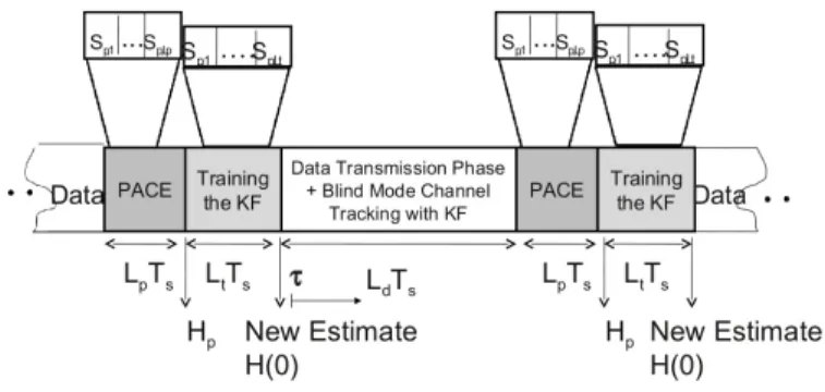
Fig. 1. Alternating training and data phases in the hybrid training scheme
phase and the end of the data transmission phase, i.e. 0 ≤ τ ≤ Ld, as shown in Fig. 1. In case of channel tracking,
the PACE estimate can be used as good initial value for the tracking algorithm at the start of every training interval. A basic prerequisite is a recursive tracking algorithm, as it is the case for the KF.
Doing so, the question that arises is how good the initializa-tion has to be. In case of slow fading, increasing the number of pilots improves the PACE estimate and we can expect a faster KF convergence. However, if the channel is varying fast, the PACE estimate has to be built upon a few pilots. Therefore, we first give a deeper insight into PACE in order to determine the optimal training length. On the other hand and to the best of our knowledge, KF training in the literature is only applied to the filter itself [4], [5], [2]. In other words, the measurements from periodically sent pilots are used as input to train the statistical variables of the algorithm. Instead, we adopt a hybrid training scheme. This approach was first introduced in [6] and has proved to significantly improve the tracking performance of the RLS algorithm. Motivated by these results and the existing correspondences between RLS and KF [7], we applied the hybrid training scheme in [6] to the KF. The simulations results in Section VII confirm the expected performance improvement.
Additionally, we show that if the mean squared error (MSE) of the KF tracking at the end of the frame is smaller than the PACE MSE, the initialization with PACE is disadvantageous. In this case, pilots are not needed anymore and the KF can operate in a quasi-blind decision-directed mode. Due to the KF sensitivity to wrongly detected data, pilots have still to be requested in case of error propagation, which we introduce as a new aperiodical, pilot-on-request training scheme.
III. PILOT-ASSISTEDCHANNELESTIMATION
During the training phase, pilot symbol vectors sp,i with
1 ≤i≤Lp are transmitted. The corresponding receivedyp,i
are impaired by AWGN vectors wp,i. From (1) follows:
yp,i=Hsp,i+wp,i for 1≤i≤Lp. (3)
Assembling all pilot symbol vectors sp,i, all corresponding
receive symbol vectors yp,i as well as wi in matrices and
assuming that the channel does not change during the PACE
training phase, we get
Yp=HSp+Wp. (4) with Sp = [sp,1 · · · sp,Lp , Yp = [yp,1 · · · yp,Lp and Wp = [wp,1 · · · wp,Lp
. The PACE estimate is computed upon the received pilots according to
ˆ
HM Lp =Yp·SHp · SpSHp
−1
(5) for the ML estimate, where(.)H refers to the Hermitian of a
matrix. If knowledge about the SNR and the channel spatial correlation properties is available at the receiver, a better PACE estimate can be computed according to the MMSE principle. Therefore, we rewrite (4) in vector form to apply standard results from estimation theory:
vec(Yp) | {z } ˆ yp = STp ⊗I | {z } Xp ·vec(H) | {z } h +vec(Wp) | {z } ˜ w (6)
where ⊗ is the Kronecker product. The MMSE estimate ˆ
hM M SEp =vec(HˆM M SEp )is given by: ˆ hM M SEp =RhhXHp XpRhhXHp +Rw ˜˜w −1 ˜ yp (7) where Rhh = E hhH and Rw ˜˜w = E n ˜ w ˜wHo. When using PACE for the initialization of the tracking algorithm, we have to get a deeper insight into its estimation quality. An appropriate means to do so is to consider the channel estimation MSEζ(τ), which we define throughout this paper by: ζ(τ) = 1 M NE n kH(τ)−Hˆk2F o (8) where k · kF is the Frobenius norm andHˆ =Hˆpin case of PACE. We now take account of the channel time variations during the training phase. With orthogonal training data , i.e. SpSHp =LpIM and the channel according to (2), we derive
the ML mean squared estimation error as in (9)1. A similar
expression was derived in [8] but only for one tx antenna. Our expression holds for an arbitrary numberM of tx antennas.
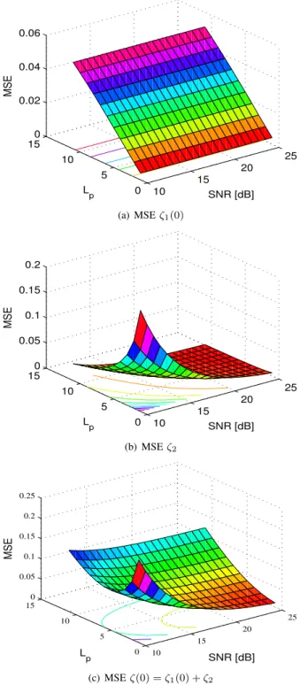
ζ(τ) = M L2 p Lp X i=1 ξ(i, τ) | {z } ζ1(τ) +2σ 2 0 Lp |{z} ζ2 (9) where ξ(i, τ) = 2(1 −J0(2πfd(τ +Lp −i))). (9) shows
that the PACE MSE is composed of two quantities: ζ1(τ)
depending on the channel time variance andζ2which is related
to the AWGN. We see that increasing the number of pilotsLp
decreases ζ2 but may increase ζ1(τ). Especially for high fd
and depending on the SNR an optimalLp that minimizes (9)
exists. This is illustrated in Fig. 2, whereζ(0)is plotted as a function of the SNR andLpforfd= 0.02.τ= 0is considered
sinceζ(0)is of interest when using PACE for the initialization of the tracking algorithm.
1For space reasons, we only giveζ(τ)for ML estimation.ζ(τ)for the
If we use the approximation J0(x)≈1−x2/4 for x≪1,
and set the first derivative of (9) with respect toLpto zero, the
optimal training length which minimizes (9) can be derived to:
Lp,opt= ( jq 1 2+ 3σ2 0 π2f2 dM k if q 1 2+ 3σ2 0 π2f2 dM > M M otherwise (10) where ⌊·⌋refers to the floor operation. (10) shows thatLp,opt
increases with increasingσ2
0and decreases with increasingfd
orM. We should keep in mind thatLp≥M must be satisfied
which is a necessary condition for the inversion in (5).
10 15 20 25 0 5 10 15 0 0.02 0.04 0.06 SNR [dB] L p MSE (a) MSEζ1(0) 10 15 20 25 0 5 10 150 0.05 0.1 0.15 0.2 SNR [dB] Lp MSE (b) MSEζ2 10 15 20 25 0 5 10 15 0 0.05 0.1 0.15 0.2 0.25 SNR [dB] Lp MSE (c) MSEζ(0) =ζ1(0) +ζ2
Fig. 2. PACE MSE as function of SNR andLpforfd= 0.02
IV. THEKALMANALGORITHM
If the fading channel can be modeled as an autoregressive process of orderp(AR(p)), then the KF is the optimal MMSE estimator. However, since the first few channel correlation terms in (2) are basically important for symbolwise tracking, AR(2) modeling is adopted in this work as in [1]. The Kalman algorithm relies on a state-space formulation composed of the observation equation (11) and the process equation(12).
y(n) =X(n)·z(n) +w(n) (11)
z(n) =Fz(n−1) +Bu(n) (12)
wherez(n) = [hT(n) hT(n−1) · · · hT(n−p+1)]T
withh(n) =vec(H(n))andFis the state transition matrix. X(n) contains the detected symbol vector ˆs(n) according to X(n) = [ˆs(n)⊗IN ON×N M(p−1)]. u is the driving
noise with E[u(n)u(n)H] =I
M N 2. We briefly list the key
equations of the Kalman tracking algorithm:
• Predicted channel state
ˆz(n|n−1) =Fzˆ(n−1|n−1) (13) • Predicted MSE P(n|n−1) =FP(n−1|n−1)FH+BBH (14) • Kalman Gain K(n) =P(n|n−1)XH(n)· X(n)P(n|n−1)XH(n) +Rww −1 (15)
• Corrected channel state
ˆ
z(n|n) = ˆz(n|n−1)+K(n)(y(n)−X(n)ˆz(n|n−1)) (16)
• Corrected MSE
P(n|n) = (I−K(n)X(n))P(n|n−1) (17) Some initial values for ˆz(0|0) and P(0|0) must be chosen to launch the algorithm, the so-called starting conditions. So far in the literature the starting conditions are set to arbitrary values or to the mean value of the corresponding variable if known [5]. By means of replacing actual data by training symbols (full training), we can find the amount of training needed for convergence of the filter. The full training analysis reveals that the convergence can be dramatically accelerated by choosing more appropriate starting conditions.
According to the initialization of the algorithm, we differ-entiate between two periodical training schemes: A scheme where onlyˆz(0|0)is trained by means of PACE, called “con-ventional periodical training” (CPT), and a “hybrid periodical training” (HPT), where both variablesˆz(0|0) andP(0|0) are trained. Both schemes will be discussed in the next section.
2FandBhave to be computed depending on the AR process order p such
that (2) is fulfilled. In the following they are assumed to be known at the receiver. Please refer to [1] for explicit definition.
V. PERIODICALTRAINING OF THEKALMANTRACKING
ALGORITHM
As can be seen in Fig. 1, the periodically sent pilots are divided into two sequences. One sequence of lengthLpthat is
attributed to the PACE block provides the tracking algorithm with a good initial estimate. The second sequence trains the algorithm and takes LtTs time. For a fair comparison of the
new training scheme with the previously established ones, the optimalLp andLtare chosen such that(Lp+Lt)/Ld is kept
constant.
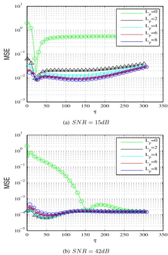
In order to study the convergence of the KF, Fig. 3 and Fig. 4 plot the MSE ζ(τ)in case of full training. The performance of the tracking algorithm depends highly on the quality of the initialization. In case of initialization with zero, the filter might even not converge within a frame. The convergence is however drastically accelerated if an amount of the training data is spent on more appropriate initialization with PACE.
0 50 100 150 200 250 300 350 10−2 10−1 100 101 τ MSE L p=0 L p=2 L p=4 L p=6 L p=8 (a)SN R= 15dB 0 50 100 150 200 250 300 350 10−3 10−2 10−1 100 101 τ MSE L p=0 L p=2 L p=4 L p=6 L p=8 (b)SN R= 42dB
Fig. 3. Channel estimation MSEζ(τ)for full training with differentLpat fd= 0.01
The full training analysis leads to a further result. In the steady state at the end of a frame, the MSE can be smaller than the PACE MSE at the beginning of a frame, i.e.ζ(Ld)< ζ(o).
This happens for example in the desicion-directed mode at high SNR when the detected data is mostly correct. In this case, reinitializing the algorithm is not advantageous. There-fore, we have to think about a mechanism to decide whether to reinitialize with PACE or not. The theoretical PACE MSE (9)
0 50 100 150 200 250 300 350 10−3 10−2 10−1 100 101 τ MSE L p=0 L p=2 L p=4 L p=6 L p=8 (a)SN R= 15dB 0 50 100 150 200 250 300 350 10−5 10−4 10−3 10−2 10−1 100 101 τ MSE L p=0 L p=2 L p=4 L p=6 Lp=8 (b)SN R= 42dB
Fig. 4. Channel estimation MSEζ(τ)for full training with differentLpat fd= 0.001
and the error covariancePprovide us with an efficient tool to do so. If the theoretical MSE is much smaller than the trace of P, reinitialization makes sense. Otherwise, the received pilots are not needed. Because of the periodical training, this means that pilots are transmitted at the beginning of each frame but are not used which is a real waste of bandwidth. This leads us to the aperiodical training scheme where pilots are only sent when needed, i.e on request. The pilot on request training scheme (PRQT) is discussed in the next section.
VI. APERIODICALTRAINING: PILOTS ONREQUEST
In this training scheme, pilots are transmitted on request3.
The necessity for pilots arises when the Kalman filter diverges as a consequence of a series of detection errors. KF works robustly as long as the detected symbols are almost correct. In case of misdetections the model in (11) is not matched anymore and the channel estimation quality deteriorates which may result in more misdetections in the following steps and to error propagation. Accurate detection of error propagation is a key issue for the novel PRQT in order not to impair the spectral efficiency.
3We assume that the transmission of the pilots is delay-free. Consideration
of a stochastically delayed time of arrival of the receive pilot signal is subject to future work.
0 500 1000 1500 2000 2500 −2 0 2 true real h11(n) estimated real h 11(n) 0 500 1000 1500 2000 2500 0 1 2x 10 −3 tr(P(n|n−1)) tr(P(n|n)) 0 500 1000 1500 2000 2500 0 0.005 0.01 tr(R ee(n)) 0 500 1000 1500 2000 2500 0 1 2 |e(n)|2
Fig. 5. Analysis of different variables in the KF as function of the discrete timen
In [2], [9] reliability information about the detected data is used to detect wrongly detected symbols and exclude them from channel tracking. This approach is feasible as long as the channel is almost invariant on a received block. Besides, it requires an iterative receiver that can provide statistical reliability information. Instead, if symbolwise tracking with a non-iterative receiver is required due to fast fading, this scheme is not applicable anymore and we have to think of other indicators for the error propagation.
Closer analysis of different statistical quantities involved in the KF algorithm suggests that a filter divergence occurs in most of the cases just after a steep peak has appeared in their progress. This is for example the case for the magnitude of the innovation processe(n) =y(n)−X(ˆ n)ˆz(n|n−1). However, other variables such as P(n|n−1), P(n|n), and Ree(n)
remain unchanged.Ree(n)is the covariance of the innovation
defined by Ree(n) = E[e(n)e(n)H]. Further mathematical
manipulations on Ree yield (18). Computation of (18) is
performed within the Kalman gain in (15) at each iteration and therefore does not require any further computational resources. Ree(n) =X(n)P(n|n−1)XH(n) +Rww (18)
Fig. 5 shows some variables involved in the KF tracking process for fd = 0.004, Lt = 2and Ld = 200. We can see
that a large |e(n)| due to an instantaneous high noise value gives birth to a filter divergence. The error propagates until the beginning of the next frame where the divergence is interrupted by setting the estimate to the PACE value.
Armed with these observations, we develop a first metric
m1 to detect a filter divergence. If m1 = |e(n)| exceeds a
threshold Qthwhich is related to the expectation in (18), an
error propagation is occuring and pilots are requested to stop it. Intuitively, Qth is expected to depend on the SNRγdB. If Qth is small, we would be requesting and transmitting pilots
all the time instead of data, reducing the spectral efficiency. On the other hand, a large Qth can fail in detecting many
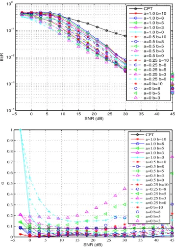
−5 0 5 10 15 20 25 30 35 40 45 10−4 10−3 10−2 10−1 100 SNR (dB) BER CPT a=1.0 b=10 a=1.0 b=8 a=1.0 b=5 a=1.0 b=3 a=1.0 b=0 a=0.5 b=10 a=0.5 b=8 a=0.5 b=5 a=0.5 b=3 a=0.5 b=0 a=0.25 b=10 a=0.25 b=8 a=0.25 b=5 a=0.25 b=3 a=0.25 b=0 a=0 b=10 a=0 b=8 a=0 b=5 a=0 b=3 −5 0 5 10 15 20 25 30 35 40 45 0 0.1 0.2 0.3 0.4 0.5 0.6 0.7 0.8 0.9 1 SNR (dB) α CPT a=1.0 b=10 a=1.0 b=8 a=1.0 b=5 a=1.0 b=3 a=1.0 b=0 a=0.5 b=10 a=0.5 b=8 a=0.5 b=5 a=0.5 b=3 a=0.5 b=0 a=0.25 b=10 a=0.25 b=8 a=0.25 b=5 a=0.25 b=3 a=0.25 b=0 a=0 b=10 a=0 b=8 a=0 b=5 a=0 b=3
Fig. 6. BER as function of the SNR for various(a, b)(top). Ratio pilots over dataαas function of the SNR for various(a, b)(bottom)
error propagations. Thus, finding the optimal threshold is a constrained optimization problem. We have to search for the threshold that minimizes the BER under the constraint that the spectral efficiency remains beyond a certain value. Out of lack of mathematical tractability for this problem and for the sake of simplicity,Qth is defined as an affine function of γdB by
means of the coefficientsaandb as follows:
Qth= (a·γdb+b)
p
tr{Ree} (19)
By intensive simulations, we determine the coefficientsaand
b which minimize the BER keeping the spectral efficiency beyond a certain value. To evaluate the quality of spectral efficiency, we introduce the parameter α which denotes the ratio of number of pilots over data. Some results of this optimization process are illustrated in Fig. 6. Therein, the trade-off between small BER and large spectral efficiency is plain to see. For instance,(a, b) = (0,3) leads to the lowest BER but the required number of pilots is very high. On the other hand, (a, b) = (1,10)requires the smallest number of pilots but at the expense of large BER.
As a second approach, we suggest to consider the normal-ized innovation squared (NIS), in order to provide a metric
m2 independent of the SNR. The NISm2 is defined as:
−5 0 5 10 15 20 25 30 35 40 10−4 10−3 10−2 10−1 100 SNR (dB) BER HPT PRQT M d=10 PRQT M d=18 PRQT M d=23 PRQT M d=30 PRQT M d=40 PRQT M d=50 PRQT M d=100 PRQT M d=200 PRQT M d=500 PRQT M d=1000 −5 0 5 10 15 20 25 30 35 40 45 10−6 10−5 10−4 10−3 10−2 10−1 100 SNR (dB) α HPT PRQT M d=10 PRQT M d=18 PRQT M d=23 PRQT M d=30 PRQT M d=40 PRQT M d=50 PRQT M d=100 PRQT M d=200 PRQT M d=500 PRQT M d=1000
Fig. 7. BER as function of the SNR for variousMd(top). Ratio pilots over dataαas function of the SNR for variousMd(bottom)
An error propagation occurs if m2 exceeds a threshold
Md. This approach is known as “validation gating” and
is widely known in the field of target tracking to exclude very unlikely measurement-to-track associations [10]. The NIS follows a chi-square probability density function. Thus e(n)HR−1
eee(n)< Md means that for a probability that p%
of true associations are accepted, Md can be computed from p 100 =P( N 2 , Md 2 ) = 1 Γ(N/2) Z Md/2 0 e−ttN/2−1dt (21) whereΓis the Gamma function. For instance, forp= 99,99% and N = 2, Md = 18.42. The BER for different Md values
and the correspondingαare illustrated in Fig. 7. The trade-off between low BER and high spectral efficiency is again plain to see.
VII. SIMULATIONRESULTS
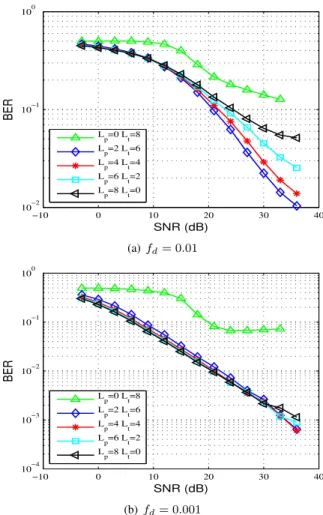
A 2×2 MIMO system with BPSK modulation and zero-forcing receiver is considered. We assume that a constant spectral efficiency is given. This means that for periodical training, we keep the ratio of training and data transmission phase lengthsα= (Lp+Lt)/Ldconstant. For our simulations,
we take Ld= 100andLp+Lt= 8. The corresponding BER
results for HPT with differentfdare illustrated in Fig. 8. These
results suggest that training the algorithm exclusively performs worse than allocating an amount of the training to supply the algorithm with a PACE initialization for bothfd. Furthermore,
we notice that HPT with Lp = 2, Lt = 6 performs best
for fd = 0.01. Indeed, at fd = 0.01, Lp = 2 leads to the
smallest PACE MSE. At smaller fd, investing all pilots for
PACE initialization leads to the lowest BER on the whole considered SNR range. −10 0 10 20 30 40 10−2 10−1 100 SNR (dB) BER Lp=0 Lt=8 Lp=2 Lt=6 Lp=4 Lt=4 Lp=6 Lt=2 Lp=8 Lt=0 (a)fd= 0.01 −10 0 10 20 30 40 10−4 10−3 10−2 10−1 100 SNR (dB) BER L p=0 Lt=8 L p=2 Lt=6 L p=4 Lt=4 L p=6 Lt=2 L p=8 Lt=0 (b)fd= 0.001
Fig. 8. BER as function of the SNR for hybrid training scheme withLp+ Lt= 8
The BER results for PRQT, optimized under the constraint thatα≤8%for comparison fairness, are plotted in Fig. 9 for
fd = 0.01. PRQT with both suggested metrics outperforms
CPT and HPT significantly. The ratio of required pilots is even reduced to less than 2% as can be seen in Fig. 10. For PRQT with m2, Md = 30 is chosen for an SN R < 24dB
and Md = 50 beyond since this yields to a good trade-off
between BER and spectral efficiency, respecting the constraint
α ≤ 8% on the whole considered SNR range. PRQT with
m2 outperforms PRQT with m1 for SN R <12dB. For low
SNR however, it leads to similar BER as for CPT and HPT. The discontinuities in Fig. 10 arise from adopting different parameters ((a, b)for m1, and Md for m2) depending on the
SNR. Considering that it is less complicated to optimize the threshold Md in comparison to Qth (2 degrees of freedom
with the coefficientsaandb), the NIS metricm2 is preferred
−5 0 5 10 15 20 25 30 35 40 45 10−5 10−4 10−3 10−2 10−1 100 SNR (dB) BER CPT Lp=8 Lt=0 CPT Lp=0 Lt=8 HPT Lp=2 Lt=6 CPT Lp=8 Lt=0 perfect decoding PRQT m1 PRQT m2 perfect CSI
Fig. 9. BER as function of the SNR for CPT, HPT, PRQT and perfect CSI
−5 0 5 10 15 20 25 30 35 40 45 10−3 10−2 10−1 SNR (dB) α CPT, HPT L p+Lt=8 PRQT m 1 PRQT m 2
Fig. 10. Ratio pilots over dataαfor PRQT and CPT with 8% training
A further very remarkable result is that the BER curves for KF with PRQT and KF operating with CPT and per-fect detection are overlapping between 12dB and 36dB. For SNR<12dB, PRQT generally performs worse due to the constraint of spectral efficiency. In the high SNR however, it even outperforms the tracking with perfect detection. The performance gap between PRQT and perfect CSI is basically due to the model mismatch with AR(2). We expect this gap to be smaller with higher AR order.
VIII. CONCLUSION
In this paper, we deal with tracking fast-varying MIMO channels by applying the Kalman algorithm. Different training schemes for this algorithm are suggested such as the hybrid periodical scheme and the pilot on request scheme. They are compared to the conventional periodical training. The hybrid scheme can decrease the BER floor by an order of magnitude in comparison to the conventional periodical training while maintaining the same spectral efficiency. For the aperiodical pilot on request training, we develop two different metrics for detecting the error propagation. Finally, we show that with the novel training on request scheme the BER can be significantly decreased while the number of required pilots is remarkably reduced.
REFERENCES
[1] C. Komninakis, C. Fragouli, A. Sayed, and R. Wesel, “Multi-input multi-output fading channel tracking and equalization using Kalman estimation,” IEEE Transactions on Signal Processing, vol. 50, no. 5, pp. 1065 –1076, May. 2002.
[2] I. Nevat and J. Yuan, “Joint channel tracking and decoding for BICM-OFDM systems using consistency tests and adaptive detection selection,”
IEEE Transactions on Vehicular Technology, vol. 58, no. 8, pp. 4316 –4328, Oct. 2009.
[3] J. Choi, M. Bouchard, and T. H. Yeap, “Adaptive filtering-based iter-ative channel estimation for MIMO wireless communications,” IEEE International Symposium on Circuits and Systems, pp. 4951 – 4954 Vol. 5, May. 2005.
[4] E. Karami and M. Shiva, “Decision-directed Recursive Least Squares MIMO Channel Tracking,”EURASIP Journal on Wireless Communica-tions and Networking, Dec. 2005.
[5] S. Haykin,Adaptive Filter Theory. Prentice-Hall, Inc., 1996, ISBN 0-13-322760-X.
[6] E. Eitel, R. A. Salem, and J. Speidel, “Improved decision-directed recursive least squares MIMO channel tracking,” IEEE International Conference on Communications, pp. 1 –5, Jun. 2009.
[7] A. Sayed and T. Kailath, “A state-space approach to adaptive RLS filtering,”IEEE Signal Processing Magazine, vol. 11, no. 3, pp. 18 –60, Jul. 1994.
[8] Q. Sun, D. Cox, H. Huang, and A. Lozano, “Estimation of continuous flat fading MIMO channels,”IEEE Transactions on Wireless Communi-cations, vol. 1, no. 4, pp. 549–553, Oct. 2002.
[9] I. Nevat and J. Yuan, “Channel tracking using pruning for MIMO-OFDM systems over Gauss-Markov channels,”IEEE International Conference on Acoustics, Speech and Signal Processing, vol. 3, pp. III–193 –III– 196, Apr. 2007.
[10] T. Bailey, B. Upcroft, and H. Durrant-Whyte, “Validation gating for non-linear non-Gaussian target tracking,”9th International Conference on Information Fusion, pp. 1 –6, Jul. 2006.