Parabolic Trough Solar Collector Analysis
Derek Lipp
AME 40463
Capstone Design Project
28 February 2008
Abstract
The purpose of this trade study is to examine a parabolic trough and determine the ideal width and focal length given constraints on the amount of light available, the length of the trough, and reflector material properties. It will show for a 48 inch heat collection element and Southwall’s Silver-BSR, the ideal width is 50 inches and the ideal focal length is 5.75 inches given South Bend, IN solar radiation.
1
Developing the Trough Characterization
The problem presented is to determine the ideal width and focal length of a parabolic trough. In order to do this, we must first develop the mathematical characterization of the trough and rays incident upon it, shown in Figure 1 provided the parabolic equationy= x2
4f
1
, where
f is the focal length of the parabola. The rays incident upon the trough are assumed to be parallel due to the sun’s approximately infinite distance, and at perfect alignment, these rays are parallel to the y-axis. The slope of the trough is tanθ such that,
tanθ = dy dx = x 2f →θ= tan −1 x 2f .
The normal at an arbitrary value of x bisects the incident ray and its reflection, and the incident ray is shown to be perpendicular to the x-axis. This observation coupled with the
1Price, et al., 2002, ”Advances in Parabolic Trough Solar Power Technology”, ASME Journal of Solar
n^ t^ y = 4f x2 y* y x β θ θ θ y θ Parabola f Focus Reflection
Incident light ray
Figure 1: The geometric definition of the simple case. n ^ t^ f* y x β ψ θ φ y y*
Figure 2: The geometric definition includ-ing misalignment
definition of y∗ (shown in Figure 1) yields,
y∗ =f∗−y =xtanβ → (1)
f∗ =xtanβ+y (2)
In Equations 1 and 2, f∗ is the y coordinate where the incident light is reflected to, and mathematically β = π
2 −2θ. In Figure 1, f and f∗ are equal, while in Figure 2, f∗ > f.
Introduce a misalignment, φ, and variable ψ and re-derive y∗ and f∗ according to Figure 2. Algebraically, this is represented by,
ψ =θ−φ β = π 2 −ψ−θ= π 2 −2θ+φ y∗ =xtanπ 2 −2θ+φ =xtan π 2 −2 tan −1 x 2f +φ (3)
With the expanded definition of Equation 1 seen in 3, Equation 2 becomes Equation 4.
f∗(x, f, φ) =xtan π 2 −2 tan −1 x 2f +φ + x 2 4f. (4)
As seen in Equation 4, f∗, is a function of the x coordinate of the trough, the focal length,
f, and any misalignment of the trough from perfect alignment,φ.
2
Considerations for Variables of the Trade Study
The design of the parabolic trough is defined by four main characteristics: the width, the length, the focal length, and the reflective material. For the present study, the length was constrained to 48 inches by the choice of an evacuated glass solar tube. Due to time constraints, a reflective material was chosen based on a response to an inquiry concerning Southwall Technologies’ Silver-BSR (data sheet provided in Appendix) material2
. Design requirements state that the system must run given solar radiation typical to South Bend, IN. Using NOAA data for the month of December, this was found to be 260W
m2.
The design of the parabolic trough produces a number of state variables including, the power output, the incident area of light, the amount of material needed, the cost, the motion envelope, and the losses from misalignment. By a simple energy efficiency calculation involving approximate generator, engine, and heat transfer efficiencies, power output was determined to be 423.28 W. The incident area of light is the projection of light hitting the trough onto a plane (A = cosφ·L·W), and when φ is small, cosφ ≈ 1. φ was limited to less than four degrees, because preliminary results revealed losses from greater values of φ
were near 100%. The total cost of the material is dependent on the amount needed. The final state, and merit of the project, generated is the loss due to misalignment, with minimal losses being desirable.
At this time, note the limitations of the study. This study is meant to examine trends in data produced from the derivation and not intended as final design criteria. The final numerical results for this study apply solely to the material stated above and are theoretical based on the aforementioned and derived analysis. Results are generated assuming perfect alignment can be achieved. Furthermore, validation of this study through experimentation
should be considered to account for scattering affects of the reflective material, manufacturing imperfections and misalignments greater than the studied range (0◦ < φ <4◦).
3
Results
The following is the development and results of the trade study for the Southwall Silver-BSR material. Given a full spectrum (above 50 nm) reflectance of 94%, the length of 48 inches, available power of 260W
m2, and required power output of 423.28 W yields a necessary width from the following balance:
m2 260W · 1in 0.0254m 2 · 1 48in ·0.94·423.28W = 49.41in→ width 2 ≈25in
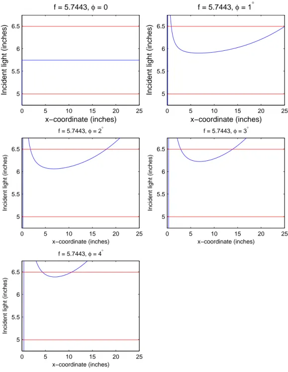
Now recall Equation 4, and from above the x range was 0 < x < 25 inches and the range of misalignment was 0 < φ < 4◦. The remaining design variable, focal length, was initially tested from 1 < f < 19 inches in increments of two inches. Loss was calculated as the percentage of rays falling outsidef±0.75 inches (the radius of inner, absorbent tube). This method can be seen graphically in Figure 3 as the reflected light position (blue line) plotted within the range of working values (red lines).
φ(◦) losses (%) 0 0 1 3.48 2 34.75 3 55.10 4 74.05
After examining data from the initial run, minimal losses were seen to lie within a focal length range of three to thirteen inches (see MATLAB terminal output in the Appendix). The search parameters were refined to reflect this new range and discretized to increments of 0.01 inches and degrees for the focal length and misalignment respectively. Finally, values for the focal length with minimal loss were weighted to calculate the ideal focal length. Running this new simulation code (in the Appendix) revealed the ideal focal length to be 5.7443≈ 5.75 inches. This focal length produces the accompanying table of losses (seen
0 5 10 15 20 25 5 5.5 6 6.5 x−coordinate (inches)
Incident light (inches)
f = 5.7443, φ = 0 0 5 10 15 20 25 5 5.5 6 6.5 x−coordinate (inches)
Incident light (inches)
f = 5.7443, φ = 1° 0 5 10 15 20 25 5 5.5 6 6.5 x−coordinate (inches)
Incident light (inches)
f = 5.7443, φ = 2° 0 5 10 15 20 25 5 5.5 6 6.5 x−coordinate (inches)
Incident light (inches)
f = 5.7443, φ = 3° 0 5 10 15 20 25 5 5.5 6 6.5 x−coordinate (inches)
Incident light (inches)
f = 5.7443, φ = 4°
graphically in Figure 3).
4
Impact of Results
As expected from Equation 4 and confirmed by examining output over ranges of x, the ideal focal length varies sinusoidally. This was noted early in the development process and thus the values were simply evenly weighted to give a single output value. A more complex weighting method could be developed and used to account for larger retained incidence from smallxvalues where losses are minimal. This may also be used to account for the trend that a focal length greater than the ideal is preferred over a focal length shorter than the ideal, since the latter produces higher losses. With this in mind, the general trend in focal length is to increase as the overall width of the trough increases. This could be used to redimension the trough if a longer or shorter heat collection element is used, since the necessary width is linearly proportional with the amount of energy required of the unit.
Results indicate a larger trough than initially conceived but at 1.548 square meters remains under the two square meters limit. The ability to easily solve for an ideal focal length given a necessary width (determined by material reflectivity) as demonstrated by the MATLAB script, is encouraging for future material changes that the project may encounter. A negative result is the essentially four degree limit of misalignment revealed in the results. This means an accurate alignment system with tight tolerances will be required to maximize the benefits of the trough.
5
Additional State Information
Two additional pieces of state information were generated with the information from the study. To find the surface area of reflective material needed for the trough, recall the line
integral for the parabola, Aref lector = 2 Z 2 0 5 r 1 + x 2 4·5.752 dx·48 = 3709.8in 2
Provided a cost of $0.004516 per square inch courtesy of Mr. Coda, the final state is a reflector cost of $16.76.
6
Appendix
6.1
MATLAB code
%Derek Lipp
%Solar Power Parabolic Trough Trade Study %12 February 2008
%Code to examine the optical properties of parabolic troughs as
%characterized by the accompanying development and geometric derivations %This specialized version developed from a generic version
close all clear all clc
%dimensions given per inch
%specify target focal lengths and deviation from incidence focal = [3:.01:13]; phid = [0 1 2 3 4]; phi = phid.*pi/180; widths = [25]; for z = 1:1 %specify x-values width = widths(z); x = [0:.01:width]; parameter = width*100+1;
%%%%% Loop for testing multiple values of widths and focal lengths %%%%%% % for i = 1:1001
% for k = 1:41
% count = 0;
% for j = 1:parameter
% y_star(j) = x(j)*tan(pi/2 - 2*atan(x(j)/2/focal(i)) + phi(k))
% + x(j)^2/4/focal(i); % if abs(focal(i)-y_star(j)) > .76 % count = count + 1; % end % end % loss(i,k) = count/parameter; % end
% end % % ideal = 0; % k = 2; % for i = 2:41 % for j = 2:1001 % if loss(j,i) < loss(j-1,i) % k = j; % end % end
% ideal = focal(k)/40 + ideal;
% end % best(z) = ideal; % % end % widths % best
% code to plot results of the ideal case focal(1) = 5.7443;
for i = 1:1 for k = 1:5
count = 0;
for j = 1:parameter
y_star(j) = x(j)*tan(pi/2 - 2*atan(x(j)/2/focal(i)) + phi(k)) + x(j)^2/4/focal(i); if abs(focal(i)-y_star(j)) > .76 count = count + 1; end end loss(i,k) = count/parameter; y_min = focal(i) - .75; y_max = focal(i) + .75; one = ones(1,parameter); figure plot(x,y_star) hold on plot(x,y_min.*one,’r’) plot(x,y_max.*one,’r’) end end end
6.2
MATLAB “losses” Printout
This sample printout is loss values in terms of percentage divided by 100. Values ofφincrease across the columns from left to right and values of focal length increase down the rows.
loss = Columns 1 through 6 0.0004 0.0012 0.0024 0.0032 0.0384 0.1140 0.0004 0.0012 0.0024 0.0032 0.0364 0.1124 0.0004 0.0012 0.0024 0.0032 0.0344 0.1108 0.0004 0.0012 0.0024 0.0032 0.0324 0.1088 0.0004 0.0012 0.0024 0.0032 0.0304 0.1068 0.0004 0.0012 0.0024 0.0036 0.0284 0.1052 0.0004 0.0012 0.0024 0.0036 0.0264 0.1032 0.0004 0.0012 0.0024 0.0036 0.0240 0.1012 0.0004 0.0012 0.0024 0.0036 0.0220 0.0996 0.0004 0.0012 0.0024 0.0036 0.0200 0.0976 0.0004 0.0012 0.0024 0.0036 0.0180 0.0956 0.0004 0.0012 0.0024 0.0036 0.0164 0.0940 0.0004 0.0012 0.0024 0.0036 0.0144 0.0920 0.0004 0.0012 0.0024 0.0036 0.0124 0.0904 0.0004 0.0012 0.0024 0.0036 0.0104 0.0888 0.0004 0.0012 0.0024 0.0036 0.0084 0.0868 0.0004 0.0012 0.0024 0.0036 0.0064 0.0852 0.0004 0.0012 0.0024 0.0036 0.0048 0.0832 0.0004 0.0012 0.0024 0.0036 0.0048 0.0816 0.0004 0.0012 0.0024 0.0036 0.0048 0.0796 0.0004 0.0012 0.0024 0.0036 0.0048 0.0776 0.0004 0.0012 0.0024 0.0036 0.0048 0.0760 0.0004 0.0012 0.0024 0.0036 0.0048 0.0740 0.0004 0.0012 0.0024 0.0036 0.0048 0.0724 0.0004 0.0012 0.0024 0.0036 0.0048 0.0704 0.0004 0.0012 0.0024 0.0036 0.0048 0.0688