Vol. 1, No. 2, pp 151-170 Summer 2007
A Comparative Study of Exact Algorithms for the Two Dimensional Strip
Packing Problem
Abdelghani Bekrar
*, Imed Kacem and Chengbin Chu
ICD-LOSI, (CNRS FRE 2848)UNIVERSITE DE TECHNOLOGIE DE TROYES FRANCE
{bekrar, kacem, chu}@utt.fr ABSTRACT
In this paper we consider a two dimensional strip packing problem. The problem consists of packing a set of rectangular items in one strip of width W and infinite height. They must be packed without overlapping, parallel to the edge of the strip and we assume that the items are oriented, i.e. they cannot be rotated. To solve this problem, we use three exact methods: a branch and bound method, a dichotomous algorithm and a branch and price method. The three methods were carried out and compared on literature instances.
Keywords: Strip packing, lower and upper bound, branch and bound, dichotomous search, column generation, branch and price.
1. INTRODUCTION
The two-dimensional strip packing problem (2SP) is a well-known combinatorial optimization problem. It has several industrial applications like the cutting of rolls of paper or textile material. Moreover, some approximation algorithms for Bin Packing problems are in two phases where the first phase aims at solving a strip packing problem (see Chung et al. (1982) and Berkey and Wang (1987)).
Consider a set of n rectangular items. Each item i has width wi and height hi(i ∈ {1,..., n}). The 2SP
consists of packing all the items in a strip of width W and infinite height. Without loss of generality, we assume that the dimensions of the items and the strip are integers. The objective is to minimize the total height used to pack the items without overlapping. The orientation of items is assumed to be fixed, i.e., they cannot be rotated.
This problem is NP-hard in the strong sense (see Garey and Johnson (1979) and Martello et al. (2003)). For this reason, most of papers considering the 2SP problem are approximation algorithms. Fernandez de la Vega and Zissimopoulos (1998), Lesh et al.,(2003), Kenyon and Remila (1996) and Zhang et al. (2006) presented approximation algorithms for the strip packing problem, whereas Gomes and Oliveira (2006), Bortfeldt (2006) and Beltran et al., (2004) used meta-heuristics. Hopper and Turton (2001) provided an overview of meta-heuristic algorithms applied to 2D strip packing problem.To our knowledge, few papers studied exact algorithms to solve 2SP problem. Hifi
*
(1998) introduced the cutting/packing problem with guillotine cut and he proposed two algorithms based on a branch and bound procedure and dichotomous search. Martello et al. (2003) proposed a new lower bound and used a branch and bound algorithm to solve the problem without guillotine constraint. Recently, three papers introduced the Strip Packing problem with guillotine constraint. Cui et al. (2006) proposed a recursive branch and bound algorithm to obtain an approximate solution. A new lower bound and a branch and bound algorithm were proposed by Bekrar et al. (2006b) for the guillotine problem. Finally, Cintra et al. (2006) used the column generation method and dynamic programming to solve another variant of the problem.
In this paper we study the two dimensional strip packing problem with non-guillotine pattern. We propose exact algorithms: branch and bound algorithm, branch and price procedure and dichotomous search to solve the problem. In Section 2 we present a lower bound and an upper bound used in a branch and bound approach. In Section 3, we use the column generation that gives a tighter lower bound. To obtain an optimal solution we present a specific branching scheme used in the branch and price procedure. Section 4 presents the dichotomous algorithm. The three algorithms are tested on literature instances and the computational results are described in Section 5. Finally, we present some perspectives of our work.
2. THE BRANCH AND BOUND ALGORITHM
The first exact method that we propose is a branch and bound algorithm. It is proposed for the guillotine case (Bekrar et al. 2006b). We adapt this method to the non-guillotine case. The upper bound, the lower bound and the branching scheme used in this branch and bound are detailed in the following subsections.
2.1 The upper bound
Several papers proposed approximation algorithms for 2D Strip Packing Problem, with or without guillotine constraint (Fernandez de la Vega and Zissimopoulos (1998), Lesh et al., (2003), Kenyon and Remila (1996), Zhang et al. (2006) and Cui et al. (2006)).
We adopt the SHF heuristic proposed for the bin and strip packing problem with guillotine constraint. This heuristic was proposed previously by Ben Messaoud et al., (2003). We proposed some strategies to improve it in Bekrar et al., (2006a), and we called it BSHF. It is a generalization of the well-known two dimensional level algorithm.
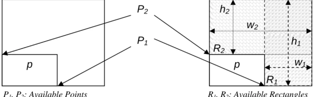
The main idea of this algorithm is to exploit the non-used area in each shelf. It makes it possible to pack items one over another in the same shelf, which is not permitted in the level algorithms.In SHF, items are packed in available rectangles (see Figure 1): the rectangles which have the bottom-left corner as an available point (see Figure 1). Such a point can be the bottom-right or the top-left
p
p
w
2h
2h
1w
1P
2P
1P1, P2: Available Points R1, R2: Available Rectangles
R
2R
1 Figure 1. Available Points and Available Rectanglescorner of an item already packed.
Items are sorted in non-increasing order of heights. The first item (the tallest one) is packed into the first available rectangle (the lowest). The leftmost item initializes a shelf with a height equal to the height of this item. After every item-packing, the set of available rectangles is updated. The updating consists of reducing the dimensions of available rectangles which overlap with the packed items. The item-packing creates two new available rectangles. This procedure is repeated until the last item is packed.
In the guillotine version of this algorithm, we tested different rules of sorting items. We used the
Best Fit rule to pack items and we proposed a new way to update the list of available rectangles. This algorithm gives good results on large instances in few seconds. The average waste rate is estimated at 9%.
2.2 Lower bounds for 2SP
In this section, we explain the lower bound used in our algorithms. First, we present some lower bounds proposed for the strip packing problem: the continuous lower bound Lc, a first lower bound
of Martello et al., (2003) which we denote by Lmmv1 and a second denoted by Lmmv2. In our
algorithms, we use our new lower bound denoted by LBKCS.
2.2.1 The continuous lower bound Lc
By splitting each item j into wjhj unit squares, we obtain a lower bound Lc which is called continuous lower bound:
⎥ ⎥ ⎥ ⎥
⎥ ⎤
⎢ ⎢ ⎢ ⎢
⎢ ⎡ =
∑
=W h w L
i n
i i
c
1
Let L0 = max {Lc, maxi=1...n hi}. Martello et al. (2003) proved that the absolute worst case
performance ratio of this bound is equal to 1/2.
2.2.2 First lower bound Lmmv1 of Martello et al., (2003)
This first lower bound presented by Martello et al., (2003) is an extension of that proposed by Martello and Toth (1990) for the one-dimensional bin packing problem.
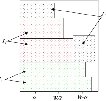
The idea is to subdivide the set of items into three sub-sets according to their dimensions. Let J be the set of items.
Let α∈ [1, W/2]
J1 = { j ∈ J: wj > W-α }, the subset of large items,
J2 = { j ∈ J : W -α≥ wj > W/2}, the subset of medium items, J3 = { j ∈ J : W/2 ≥ wj≥α }, the subset of small items,
As we can see in Figure 2:
• Beside a large item we cannot pack any item of the other subsets, • Two items of the subset J2 cannot be packed one beside the other, • Beside items of J2 only items of the class J3 can be packed.
Let:
⎟⎟ ⎟ ⎟ ⎠ ⎞ ⎜⎜
⎜ ⎜ ⎝ ⎛
⎥ ⎥ ⎥ ⎥ ⎤ ⎢
⎢ ⎢ ⎢
⎡ − −
+
=
∑
∑
∈∑
∈∪
∈ W
h w W h
w h
L j J
j j J
j j j
J J j
j
) ) (
( ,
0 max )
( 3 2
2 1
α
Lmmv1 = max1≤α≤W/2{L(α)}is a valid lower bound for the 2SP problem that can be computed in O(n log n) time (for the proof see Martello et al., (2003)).
2.2.3 Second lower bound Lmmv2 of Martello et al., (2003)
The second lower bound proposed by Martello et al., (2003) is based on a relaxation of the 2SP problem by cutting each item j∈ J into hjunit-height slices of width wj. The authors consider the one dimensional contiguous bin packing problem (1CBP), where all slices must be packed in bins of size W. The hjslices derived from the item j must be packed into hjcontiguous bins. The optimal
solution of (1CBP) is a valid lower bound for the 2SP problem (denoted by Lmmv2). This solution is
computed by a branch and bound algorithm. The authors proved that Lmmv2 dominates all the
previous lower bounds.
When the branch and bound algorithm fails to determine the optimal solution within a fixed time, a new instance of (1CBP) is created from the 2SP instance by cutting each item j ∈ J into ⎣hj/2⎦slices
W/2
W-
α
α
J
1J
2J
3of height 2, or into ⎣hj/3⎦ slices of height 3, and so on, until a solvable (1CBP) instance is
produced.Lmmv2 is improved by using a specialized binary search procedure (for more details see
Martello et al., (2003)). This lower bound gives the best results on the tested instances, but as we can remark, it is very time consuming.
2.2.4 New lower bound LBKCS
The lower bound that we use in different algorithms was proposed in our previous work for the guillotine problem. It is based on the same decomposition presented in Section 2.2.2. This bound gives good results on the same instances of Martello et al., (2003) while the computational time is lower, and the implementation is easier.
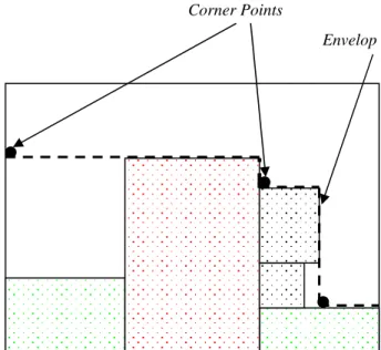
Let us consider the decomposition presented in Section 2.2.2. As we can see (Figure 3): • No item of the subsets can be packed with items of the subset J1,
• Two items of J2 cannot be packed side by side, only the items of J3 can be packed next to
J2, •
∑
∪ ∈ = 2 1 J J j j hL ,is a valid lower bound for 2SP problem.
Our idea is to calculate the maximum number of items from J3 that can be packed with items of J2, noted nps. This allowed us to compute an improved bound on the items of J3 that cannot be packed with J2. The latter bound is added to L.
J3 is sorted in non-decreasing order of area and
J
3' denotes the subset of the ( J3 −nps) smallest pieces of J3. The new lower bound is presented as:LBKCS = max1≤α≤W/2{LBKCS(α)}, where
⎟⎟ ⎟ ⎟ ⎟ ⎠ ⎞ ⎜⎜ ⎜ ⎜ ⎜ ⎝ ⎛ ⎥ ⎥ ⎥ ⎥ ⎥ ⎤ ⎢ ⎢ ⎢ ⎢ ⎢ ⎡ + =
∑
∈ − ] 3 [ ' , max ) ( 3 nps J J j j j BKCS h W h w L L αand h[j] is the height of the j th
item when sorting the items in non-decreasing order of height.
To compute nps, we use the property presented by Boschetti and Mingozzi (2003) for calculating an upper bound on the number of items that can be packed in a bin. Bekrar et al., (2006b), proposed two methods to determine the bin in which the items of J3 can be packed. A third method based on solving a knapsack problem is also used. For nps, we take the best result computed by the three methods.
2.3 The branching scheme
To solve the 2SP problem to optimality, we employ the same branching-scheme used by Martello et al. (2003). The Depth First strategy is adopted in the tree search.
At each decision, a partial solution is composed of the set of items already packed I ⊂ J. This solution is increased by selecting each item j ∈ I\J for branching, and packing them in a "feasible"
position.
Martello et al. (2000) proved that the items of I define an "envelop" that separates the two regions where the items of J\I may (resp. may not) be placed, and it is enough to generate nodes where j is placed in the "corner points" (black points in Figure 3). The "corner points" corresponding to points where the slope of the envelop changes from vertical to horizontal, and it can be determined in O(|I|log|I|) time.
From the partial solution in each node, we construct a new instance of 2SP problem. This new instance is composed from the non-packed items and items created from the packed items. The lower bounds described above are applied on this new instance to give an evaluation of the partial solution.
A new property to eliminate symmetrical pattern
In the bin packing and strip packing problem, the problem of equivalence and dominance patterns is always encountered (for more details about equivalence and dominance problem see Scheithauer(1998)). To avoid symmetrical patterns, we apply the technique used by Martello et al (2003) and our technique based on the following property:
Let n1 and n2 be two potential nodes in the search tree. If the set of the non-packed items in the two nodes is the same, and the envelops of the two nodes are identical, then the two patterns are equivalent. Before generating a new node we check if any equivalent node exists in the same level.
3. THE BRNACH AND PRICE ALGORITHM
In this section, we present another exact algorithm for the two dimensional strip packing problem. First, we use the column generation to obtain a tight lower bound, and then a specific branching
Corner Points
Envelop
scheme is used to obtain an optimal solution. The used method is an adaptation of the one proposed by Pisinger and Sigurd (2005) for solving the bin-packing case.
The column generation was applied for the first time in 1963 by Gilmore and Gomory for the one dimensional cutting stock problem. Since then it has been used for different variants of the cutting and packing problems. Vanderbeck (1999) proposed different applications of the column generation for the one dimensional cutting and packing problems. The approach was used for the three staged two dimensional bin packing problem by Puchinger and Raidl (2004) and for the two-dimensional bin packing problem with variable bin sizes and costs by Pisinger and Sigurd (2005).
The two dimensional strip packing problem can be formulated as a Set Covering problem as follows:
Let P be the set of all feasible patterns in a single bin. A feasible pattern p ∈ P is a configuration in which a set of items are packed in a single bin of width W and height Hp. The different constraints
cited above have to be respected. We introduce the binary variable xp that is equal to 1 iff the
pattern p is selected in the final solution and 0 otherwise. The objective is to minimize the total height used to pack all items. The problem is formulated by the following model:
{
}
{ }
⎪ ⎪ ⎩ ⎪ ⎪ ⎨ ⎧ ∈ ∀ ∈ ∈ ∀ ≥∑
∑
∈ ∈ P p x n i x y st x H Minimize LP p P p p ip P p p p 1 , 0 ,..., 1 1 ) (where yip is a constant equal to 1 iff the pattern p contains item i and 0 otherwise. The LP-relaxation,
{
}
⎪ ⎪ ⎩ ⎪ ⎪ ⎨ ⎧ ∈ ∀ ≤ ≤ ∈ ∀ ≥∑
∑
∈ ∈ P p x n i x y st x H Minimize RLP p P p p ip P p p p 1 0 ,..., 1 1 ) (presented by the model (RLP), gives a tight lower bound on the integer optimal solution.
The number of feasible packing may be exponential even if the number of items is small. For that reason, we use the column generation approach to solve (RLP). This method adds a new variable (pattern) at each iteration.
3.1 A column generation for the 2SP problem
In the column generation approach, we start by solving (RLP) for a restricted set of patterns. This is called restricted master problem. The restricted set is determined by solving the two dimensional strip packing problem by the heuristic presented in section 2.1. After solving the restricted problem, we look for a new feasible pattern with a minimum reduced cost.
If a column with a negative
reduced cost
is found, it is added to the restricted master problem and the process is reiterated.Otherwise, the current master solution is optimal (for more details about column generation and branch and price approaches, see Barnhart et al. (1998)).
Let πi, i ∈ {1,..., n} bethe dual variables associated to the model (RLP). The dual program of (RLP)
is given by (DRLP):
{
}
⎪
⎪
⎪
⎩
⎪⎪
⎪
⎨
⎧
∈
∀
≥
∈
∀
≤
∑
∑
= ∈n
i
P
p
H
y
st
Maximize
DRLP
i n i p i ip P p p,...,
1
0
)
(
1π
π
π
The reduced cost of the packing p ∈ P is computed by the equation:
∑
=−
=
n i i ip pp
H
y
C
1
π
.If Cp≥ 0 for all p ∈ P’, where P’ is the set of the remaining patterns, then the solution is optimal for
(RLP). Otherwise, if the reduced cost is negative, the new column can be added to the primal model. This is equivalent to add the violated constraint to the dual model (DRLP).
The problem of finding a new column with minimum reduced cost is called the pricing problem. For the strip packing problem, we look for a new feasible pattern that has a negative reduced cost. This corresponds to the two dimensional knapsack problem with respect to the bin packing constraints (no overlapping, orthogonal packing, no item rotation). We associate to each item i ∈ {1,..., n} a profit πi. The objective is to maximise the profit of the packed items in a single bin of
width W and height Hp.
To solve the pricing problem, we try to construct a feasible solution with a negative reduced cost by a greedy heuristic. If this heuristic fails to find such a solution, we apply the exact algorithm described thereafter.
Greedy heuristic to solve the two-dimensional knapsack problem
The items are sorted in non-decreasing order of the profits. At every iteration we pack the current item in the best available rectangle. Let Hi bethe height of the current solution after packing item i.
If the reduced cost of the current solution is less than that of the best solution found until now, then the current solution is saved. The heuristic is sketched in Algorithm 1below.
When the heuristic PSHF fails to find a pattern with a negative reduced cost, we solve the two dimensional knapsack problem to optimality by using the algorithm described as follows.
An exact algorithm to solve the two-dimensional knapsack problem
The two-dimensional Knapsack Problem (2KP), whose input consists of a set N={1,…,n} of “small” rectangles (items), the ith having a widthwi, a heighthj and a profitpi, and a “large”
rectangle (knapsack) of width W and height H. The objective is to pack a maximum-profit subset of the items into the knapsack, with the constraint that items do not overlap and each of them must have its edge parallel to the edge of the knapsack. 2KP is a generalization of the famous one-dimensional Knapsack Problem (KP) and it is proved to be strongly NP-hard (see Capara and Monaci (2004)). The 2KP has been widely studied in the literature. Beasley (1985), Hadjiconstantinou and Christofides(1995), Boschetti et al. (2002) and Fekete and Schepers (1997) present different upper bounds embedded into different branch-and-bound algorithms.
To solve this problem we use the technique of Fekete and Schepers (2001). It consists of splitting the problem into two sub-problems:
- An optimization problem: one dimensional knapsack problem in which we consider each item i N as an object of capacity wihi. The objective is to maximize the profits of objects packed in a
knapsack of capacity equal to WHp.
- A decision problem: we check if the items obtained by the resolution of the optimization problem can be packed in a single bin of width W and height Hp. The different constraints of bin packing
must be respected.
The one dimensional knapsack problem is formulated as follows:
Where pi is the profit of the item i, Hp is the height of the pattern p. In this model, xi is a binary
variable equal to 1 if the item i is selected in the knapsack and 0 otherwise.
-
Sort the list of the rectangles in non-decreasing order of profits.
-
RC = 0; H
s=0 ;% RC: reduced cost, Hs: height of the saved solution
-
for (i = 1 to n ) do
o
pack i in the best available rectangle
o
let H
ibe the height of the current solution, p
ibe the profit of
item i, and S be the set of the packed items
o
if (
∑
∈
−
S k k ip
H
) < RC then
RC =
∑
∈
−
S k k ip
H
,
H
s= H
i,
Save the current solution,
-
End_for
-
End.
Algorithm 1 PSHF Algorithm
{ }
i
{
n
}
x
WH
x
h
w
st
x
p
Maximize
i p i n i i i n i i i,...,
1
1
,
0
1 1∈
∀
∈
≤
∑
∑
= =The Decision Problem
The decision problem consists of checking the feasibility of the solution obtained when solving the one dimensional knapsack problem. This problem is called orthogonal packing problem (2OPP). The (2OPP) is an NP-complete decision problem (Garey and Johnson (1978)); it consistsof determining if a set of rectangles (items) can be packed into one rectangle of a fixed size (bin). Several papers studied this problem. Fekete and Schepers (2007) proposed an exact algorithm based on the graph theory. Clautiaux et al., (2006a, 2006b) proposed two approaches to solve 2OPP to optimality. The first one is a two step algorithm where they determined the x-coordinates of items in the first step, then they checked the feasibility of the obtained configurations in the second step (Clautiaux et al., (2006a)). Clautiaux et al., (2006b), used another approach based on constraint programming. The constraint programming approach was also used by Pisinger and Sigurd (2007). We choose to use the last approach in our algorithm because we have experimentally checked that it has less computational time.
The (2OPP) is solved by a constraint satisfaction program (CSP). For each pair of items i, j the domain Mijis associated. Mij= {left, right, below, above} determine the possible relative placements
among which we should choose at least one. The different relations between items can be defined as:
rij∈ Mij i, j ∈ {1, … , n}, i ≠ j rij= left ⇒ xi+wi≤ xj i, j ∈ {1, … , n}, i ≠ j rij= right ⇒ xj+wj≤ xi i , j ∈ {1, … , n}, i ≠ j
rij= below ⇒ yi+hi≤ yj i, j ∈ {1, … , n}, i ≠ j rij= above ⇒ yj+hj≤ yi i, j ∈ {1, … , n}, i ≠ j
0 ≤ xi≤ W - wi i ∈ {1, … , n}
0 ≤ yi≤ H - hi i ∈ {1, … , n}
Initially all relations rijare set to undefined.
In every iteration of the algorithm, two rectangles i and j are considered and a value is assigned to rij
from Mij. It is then checked whether a feasible assignment of coordinates exists respecting the
current relations rij. If the coordinate verification fails, the algorithm backtracks. Otherwise a
recursive call is done.
3.2 The branch and price algorithm
When we apply the column generation algorithm, it is possible that an integer solution is obtained. In such a case this solution is optimal for the two dimensional strip packing problem. Otherwise, to obtain an optimal solution for the problem, we use the branch and price approach. The branching scheme used in the branch and price algorithm must work well with the pricing problem.
Ryan and Foster (1981) used a special scheme for crew scheduling. Branching is done by dividing the solution space into two sets. In the first set two tasks r and s appear together and in the second set they must appear separately. We adapt this scheme to our problem. In the first node, two
rectangles i and j must be in the same pattern, in which case they can be combined into one object when solving the knapsack in the pricing problem. In the second node, we consider that the rectangles i and j will be in two different patterns, then a constraint xi + xj ≤ 1 is added to the
knapsack model. In each node of the branch and price tree, we apply the column generation procedure as described above until finding an optimal solution.
4. THE DICHOTOMOUS ALGORITHM
The dichotomous approach for solving packing problems was initially proposed in the well-known paper of Hifi (1998). This type of algorithm starts by computing a lower bound denoted by BI. An upper bound, denoted by BS, is then computed. If the upper bound is equal to the lower bound, then this is the optimal solution. Otherwise, we search the optimal length included in the interval [BI,
Algorithm 2 Dichotomical Algorithm
1: INPUT: n (number of items), listP (list of dimensions of items), W (Width of the strip), TimeLimit: TL
2: OUTPUT: The optimal length of the used strip
3: Subroutine: The algorithm OPP (n, L, W1, H1) that returns TRUE if the set L of n items can be packed in the bin of width W1 and height H1
4: BI := LBKCS(n, listP,W)
5: BS := BSHF(n, listP,W) 6: if (BI == BS) then 7: Return BI; STOP.
8: else If (OPP (n, listP, W, BI) == TRUE) then 9: Return BI; STOP.
10: else
11: while ((BI < BS) and (Time < TL)) do 12: If (BI - BS == 1) then 13: Return BS; STOP. 14: else S := ⎣(BS + BI)/2⎦
15: If (OPP(n, listP, W, S) == TRUE) then
16: BS := S
18: else BI := S
19: end if 20: end if 21: end while 22: end if
BS] for which the items can be packed. To reduce the search space, we use a dichotomous search. The Dichotomous Algorithm is sketched in (Algorithm 1). Here, BI is initialized by LBKCS and BS by
the heuristic BSHF described in the previous sections.
When a height S is taken from the interval [BI, BS], a decision problem is generated: could the set of items be packed in the bin of width W and height S? The problem of determining if a set of rectangles can be packed in a larger rectangle of a fixed size, is known as the two dimensional orthogonal packing problem (2OPP).
To solve (2OPP) we use the algorithm of Pisinger and Sigurd 2006). The problem and the .algorithm used to solve it are described in a previous section
5. Computational Results
All the proposed algorithms were coded in C++ and tested on a Pentium M 1.7 GHz with 1G of RAM. For the column generation and linear programs we used CPLEX and Concert Technology. The first tests were carried out on a series of small and medium instances from the literature.Those instances are available at the website of M. Hifi (http://www.laria.u-picardie.fr/hifi/OR-Benchmark/).
-Table1. Results obtained by the three algorithms for Hifi instances
-Name n W LBKCS BSHF Sbb Tbb nodes Sda Tda Scg Tcg Sbp Tbp
SCP 1 10 5 13 13 13 0.00 1 13 0.00 13 0.01 13 0.00
SCP 2 11 4 40 40 40 0.00 1 40 0.00 40 20.00 40 0.00 SCP 3 15 6 14 19 14 7.1 230269 14 403.83 13.31 333.28 19 OM SCP 4 11 6 19 23 20 2.45 79180 20 160.35 18.83 390.00 22 OM
SCP 5 8 20 20 20 20 0.00 1 20 0.00 20 0.08 20 0.00
SCP 6 7 30 38 38 38 0.00 1 38 0.00 38 0.00 38 0.00
SCP 7 8 15 12 15 14 0.01 3383 14 0.06 13.5 0.02 14 1.01 SCP 8 12 15 17 20 17 1.57 76755 17 10.45 17 4.09 17 0.00 SCP 9 12 27 68 77 68 0.14 945 68 0.01 68 2.00 68 0.00 SCP 10 8 50 78 80 80 0.18 1030 80 0.01 80 1.00 80 0.00 SCP 11 10 27 47 52 48 4.89 138513 48 0.42 48 1.00 48 0.00 SCP 12 18 81 34 38 38 3600 15914244 34 0.01 38 3600.00 38 3600.0 SCP 13 7 70 42 57 50 0.38 29361 50 0.15 50 2.00 50 0.00 SCP 14 10 100 60 83 69 15.57 471111 69 196.65 69 600.34 69 0.00 SCP 15 14 45 34 35 34 2688.13 16080100 34 445.94 34 891.51 34 0.00 SCP 16 14 6 32 35 33 606.12 23365070 33 216.83 32.5 992.03 35 OM SCP 17 9 42 39 43 34 2.07 3808 34 0.00 34 1.40 34 0.00 SCP 18 10 70 89 104 100 9.43 261879 100 97.03 97.5 43.15 100 88.25 SCP 19 12 5 26 27 26 0.01 46 26 16.36 24.2 2.74 27 OM SCP 20 10 15 19 24 20 1.73 40905 20 1.32 20 8.50 20 0.00 SCP 21 11 30 135 150 140 24.31 1058902 140 63.29 140 121.10 140 0.00 SCP 22 22 90 34 43 42 3600 45739106 39 1597.91 42.3 3600.00 43 3600.0 SCP 23 12 15 33 39 34 37.97 1675964 34 24.07 35 3600.00 39 0.00 SCP 24 10 50 103 142 109 19.34 387932 109 71.05 109 566.32 109 0.00 SCP 25 15 25 35 43 36 3600 15839980 36 657.15 40 3600.00 43 3600.0
Ave. 43.24 50.4 45.48 568.85 4855939 45.2 158.51 45.40 735.32 46.4
The second tests were carried out on instances of different sizes and different types. They are available at the website of DEIS laboratory (http://www.or.deis.unibo.it/research.html).
We compare the three methods: the branch and bound algorithm, the branch and price procedure and the dichotomous search. For each problem, Tables 1 and 2 give the following information:
Table2. Results obtained by the three algorithms for Martello et al. instances
Name n W LBKCS BSHF Sbb Tbb nodes Sda Tda Scg Tcg Sbp Tbp NGCUT01 10 10 20 25 23* 1.01 18610 23* 23.20 25 3600 25 0.00 NGCUT02 17 10 28 33 30 3600 43836217 30* 1052.72 23 127.54 33 3600 NGCUT03 21 10 28 34 28* 1621.31 19687731 28* 519.70 28 1095.91 28* 0.00 NGCUT04 7 10 17 23 20* 0.01 1953 20* 0.02 20 0.01 20* 0.00 NGCUT05 14 10 36 37 36* 0.01 204 36* 119.58 36 2275.14 36* 0.00 NGCUT06 15 10 29 36 31* 3579.01 103839866 31* 1079.26 36 3600 37 0.00 NGCUT07 8 20 20 21 20* 0.01 18176 20* 0.00 20 0.01 20* 0.00 NGCUT08 13 20 32 44 33* 55.01 999353 33* 178.06 34.14 3600 21 0.00 NGCUT09 18 20 49 64 50 3600.00 19863917 50* 1269.83 57.89 1631.31 44 OM NGCUT10 13 30 58 84 80* 198.21 13082227 80* 1152.83 67.88 1790.85 64 OM NGCUT11 15 30 50 60 52* 1058.6 15171529 52* 733.18 54 3600 84 0.00 NGCUT12 22 30 79 96 87* 3600 64961552 87* 866.32 90 3600 60 0.00 HT01 16 20 20 20 20* 0.00 1 20* 0.00 20 1712.3 20* 0.00 HT02 17 20 20 23 20* 7593 74454013 20* 378.81 21.4 3600 23 0.00 HT03 16 20 20 25 20* 25.23 624842 20* 197.53 22.56 3600 25 0.00 HT04 25 40 15 17 16 3600.00 78101161 15* 874.05 17 3600 17 0.00 HT05 25 40 15 17 15 3600.00 8027995 15* 571.65 15 2550.95 15* 0.00 HT06 25 40 15 15 15* 0.00 1 15* 0.00 15 1081.6 15* 0.00 HT07 28 60 30 33 33 3600 9672085 31* 2045.34 34.64 3600 33 0.00 HT08 29 60 30 36 35 3600 14676076 31* 1905.08 30 1546 36 3600 HT09 28 60 30 30 30* 0.00 1 30* 0.00 30 1745 30* 0.00 CGCUT01 16 10 23 25 23* 521.31 14533561 23* 323.54 23.99 2957 25 3600 CGCUT02 23 70 63 82 71 3600 32227282 67* 1219.41 78.02 3600 82 0.00 CGCUT03 62 70 636 728 676 3600 635542 676 3600.00 728 3600 728 0.00 GCUT01 10 50 1016 1016 1016* 0.00 1 1016* 0.00 1016 47 1016* 0.00 GCUT02 20 250 1133 1349 1275 3600 23863965 1251* 2214.62 1349 3600 1349 0.00 GCUT03 30 250 1803 1810 1810 3600 16936397 1810 3600.00 1810 3600 1810 0.00 GCUT04 50 250 2934 3214 3189 3600 1463787 3214 3600.00 3214 3600 3214 0.00 BENG01 20 25 30 35 35 3600 40359226 30* 608.41 35 3600 35 0.00 BENG02 40 25 57 60 60 3600 2641751 58 3600.00 60 3600 60 0.00 BENG03 60 25 84 89 89 3600 775077 86 3600.00 89 3600 89 0.00 BENG04 80 25 107 112 109 3600 381697 109 3600.00 112 OM 112 0.00 BENG05 100 25 134 138 138 3600 209982 135 3600.00 138 OM 138 0.00 BENG06 40 40 36 39 39 3600 4972538 37 2858.63 39 3600 39 0.00 BENG07 80 40 67 72 72 3600 341251 72 3600.00 72 OM 72 0.00 BENG08 120 40 101 108 108 3600 228359 102 3600.00 108 OM 108 0.00 BENG09 160 40 126 126 126* 0.00 1 126* 0.00 130 OM 126 0.00 BENG10 200 40 156 158 158 3600 243611 158 0.00 158 OM 158 0.00 Average 240.71 261.4 254.95 2375.07 15969777.32 254.13 1383.99 259.41 2605.02 259.1 300.00
N_Opt 17 27 9
- Problem name, number of items n and the width of the strip W, - Value of the lower bound LBKCSand values of the upper bound BSHF,
- Value of the branch and price solution (Sbp) and the value obtained by the column
generation (Scg),
- Value of the dichotomous algorithm solution (Sda),
- The computational time spent by the branch and bound algorithm Tbb, that of the branch and
price procedure Tbp and that of the dichotomous algorithm Tda(in seconds),
- Average: The average of time spent by each algorithm. The average value of the lower
bound, the upper bound and the number of nodes,
- N_Opt: The number of times when each algorithm reached the optimal solution,
- OM: Out of Memory given by CPLEX when solving the linear program in the branch and price algorithms is impossible.
As we can see in Table 1, the dichotomical algorithm outperforms the two other algorithms in the number of solved problems and the computational time. This algorithm solved all the instances in an average time equal to 158.51 seconds for each problem. The branch and bound algorithm solved 22 instances in an average time equal to 568.86 seconds for each problem and the branch and price solved 18 problems in an average time equal to 1291.56 seconds for each problem.
In Table 2, we present the results obtained by the different algorithms carried out on the instances of Martello et al. (2003). In this case, the performance of the dichotomous algorithm is also confirmed. As these instances are harder than the previous ones, the dichotomous algorithm could solve 27 out of 38. The branch and bound algorithm could solve 17 instances. The less efficient algorithm on these instances is the branch and price that could solve only 9 instances out of 38.
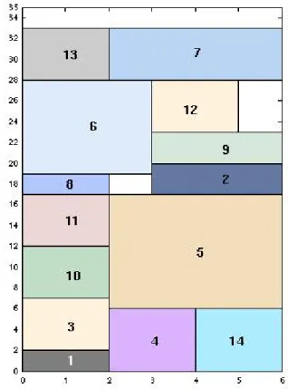
Figure 4. Optimal solution of the instance SCP16
n=14, W = 6
items hi wi
1 2 2
2 3 3
3 5 2
4 6 2
5 11 4
6 9 3
7 5 4
8 2 2
9 3 3
10 5 2
11 5 2
12 5 2
13 5 2
14 6 2
LBKCS = 32, BSHF = 35, OPT = 33 Table 3. Data of the instance SCP16.
As illustration, Figure 4 presents the optimal solution of the instance SCP16. The data of such an instance are presented in Table 3.
To analyze the performance of the algorithms to more extent, we compare the
branch-and-bound method and the dichotomous algorithm on instances randomly generated. We adapt
the classes of instances proposed by Berkey and Wang (1987)
and Martello and Vigo
(1998) for the two dimensional bin-packing problem to the strip packing problem. These
instances consist of ten classes of problems. For each class, there are 40 instances: 10 with
10 rectangles, 10 with 15 rectangles, 10 with 20 rectangles and 10 with 25 rectangles. The
first six classes have been proposed by Berkey and Wang (1987):
j = 1,…, n. n = {10, 15, 20, 25},
Class I: wj and hj uniformly random in [1, 10], W=10;
Class II: wj and hj uniformly random in [1, 10], W=30;
Class III: wj and hj uniformly random in [1, 35], W=40;
Class IV: wj and hj uniformly random in [1, 35], W=100;
Class V: wj and hj uniformly random in [1, 100], W=100;
Class VI: wj and hj uniformly random in [1, 100], W=300;
The remaining four classes were inspired b Martello and Vigo (1998). The items are
classified into the following four types:
Type 1: wj uniformly random in [2/3W, W], hj uniformly random in [1, W/2];
Type 2: wj uniformly random in [1, W/2], hj uniformly random in [2/3W, W];
Type 3: wj uniformly random in [W/2, W], hj uniformly random in [W/2, W];
Type 4: wj uniformly random in [1, W/2], hj uniformly random in [1, W/2];
The strip widths are W = 100 for all these classes, while the items are as follows:
Class VII: type 1 with probability 70%, type 2, 3, 4 with probability 10% each;
Class VIII: type 2 with probability 70%, type 1, 3, 4 with probability 10% each;
Class IX: type 3 with probability 70%, type 1, 2, 4 with probability 10% each;
Class X: type 4 with probability 70%, type 1, 2, 3 with probability 10% each;
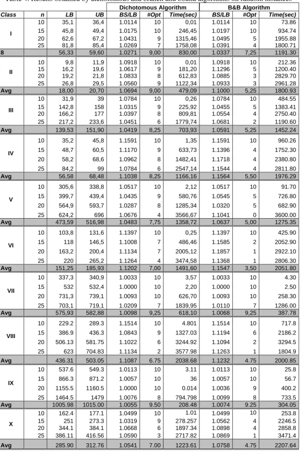
In Table 4, we present the results obtained by testing the two algorithms on randomly
generated instances. For each 10 instances, we present the average values of:
•
LB:
lower bound,
•
UB:
upper bound,
•
BS/LB
: the ratio of the best solution obtained by each algorithm on the lower
bound. Each instances was carried out for 3600 seconds (if no optimal solution was
is achieved, we take the best one),
•
#Opt
: the number of found optimum,
•
Time
: the average time spent for solving the instance.
The results shown in Table 4, confirm the results obtained previously. The dichotomous
algorithm outperforms the branch-and-bound method in the number of optimal solutions
Table 4. Results obtained by dichotomous and branch and bound algorithms on random instances
Dichotomous Algorithm B&B Algorithm
Class n LB UB BS/LB #Opt Time(sec) BS/LB #Opt Time(sec)
I
10 35,1 36,4 1.0114 10 0,01 1.0114 10 73.86 15 45,8 49,4 1.0175 10 246,45 1.0197 10 934.74 20 62,6 67,2 1.0431 9 1315,46 1.0495 5 1955.88 25 81,8 85,4 1.0269 7 1758,08 1.0391 4 1800.71
8 56,33 59,60 1.0271 9,00 830,00 1.0337 7,25 1191.30
II
10 9,8 11,9 1.0918 10 0,01 1.0918 10 212.36 15 16,2 19,6 1.0617 9 181,20 1.1296 5 1200.40 20 19,2 21,8 1.0833 8 612,83 1.0885 3 2829.70 25 26,8 29,5 1.0560 9 1122,34 1.0933 3 2961.28
Avg 18,00 20,70 1.0694 9,00 479,09 1.1000 5,25 1800.93
III
10 31,9 39 1.0784 10 0,26 1.0784 10 484.55 15 142,8 158 1.0315 9 225,92 1.0455 5 1383.41 20 166,2 177 1.0397 8 809,81 1.0554 4 2750.40 25 217,2 233,6 1.0451 6 1779,74 1.0681 2 1190.60
Avg 139,53 151,90 1.0419 8,25 703,93 1.0591 5,25 1452.24
IV
10 35,2 45,8 1.1591 10 1,35 1.1591 10 960.26 15 48,7 60,5 1.1170 9 633,73 1.1396 4 1752.30 20 58,2 68,6 1.0962 8 1482,41 1.1718 4 2380.80 25 84,2 99 1.0784 6 2547,14 1.1544 4 2811.80
Avg 56,58 68,48 1.1038 8,25 1166,16 1.1564 5,50 1976.29
V
10 305,6 338,8 1.0517 10 2,12 1.0517 10 91.70 15 399,7 439,4 1.0435 9 580,76 1.0545 5 726.80 20 564,9 593,7 1.0287 8 1285,34 1.0320 5 682.90 25 624,2 696 1.0676 4 3566,67 1.1041 0 3600.00
Avg 473,59 516,98 1.0483 7,75 1358,72 1.0637 5,00 1275.35
VI
10 103,8 131,6 1.1397 10 0,25 1.1397 10 425.90 15 118 146,5 1.1008 7 486,46 1.1585 2 2052.90 20 163,2 200,4 1.1134 7 2005,12 1.1857 1 2922.10 25 220 265,2 1.1264 4 3474,58 1.1368 1 2806.30
Avg 151,25 185,93 1.1202 7,00 1491,60 1.1547 3,50 2051.80
VII
10 337,3 340,9 1.0033 10 3,57 1.0033 10 4.30 15 532 532,4 1.0000 10 2,20 1.0000 10 2.50 20 731,3 739,1 1.0093 10 626,70 1.0093 10 258.30 25 703,1 719,1 1.0209 7 1839,95 1.0110 7 1286.00
Avg 575,93 582,88 1.0098 9,25 618,10 1.0068 9,25 387.78
VIII
10 229.2 289.3 1.1514 10 4.801 1.1514 10 717.8 15 386.9 436.3 1.0843 9 1327.03 1.1194 6 2186.2 20 506.13 581.75 1.1022 6 3244.92 1.1094 2 3294.5 25 623 704.83 1.1134 2 3577.98 1.1263 1 1804.9
Avg 436.31 503.05 1.1087 6.75 2038.68 1.1232 4.75 2000.85
IX
10 537.6 549.3 1.0113 10 3.11 1.0113 10 25.8 15 866.3 871.2 1.0057 10 36 1.0057 10 56.7 20 1155.5 1160.5 1.0000 10 0.014 1.0036 9 400.2 25 1464.5 1479 1.0076 8 794.798 1.0099 8 733.5
Avg 1005.98 1015.00 1.0055 9.50 208.48 1.0074 9.25 304.05
X
10 162.4 177.1 1.0499 10 1.01 1.0499 10 253.8 15 251 273.3 1.0319 9 278.257 1.0562 4 2246.5 20 344.1 384.1 1.0668 6 1897.34 1.0898 4 2858.8 25 386.11 416.56 1.0590 3 2717.82 1.0869 1 3471.4
found and in the average time to compute a solution. The dichotomous algorithm has been
able to solve on average more than 8 instances from 10 in every class, while the branch-and
bound procedure has been able to solve only the half of the instances.As for the two
dimensional bin packing problem, the classes of problems numbered VI, VIII and X are the
hardest problems to solve. For example, in the class VIII with n = 25 items, the
dichotomous algorithm solved only 2 problems out of 10 and the branch and bound solved
only one problem.
The easiest instances to solve are those of the classes: I, II, VII and IX. On average, 9
problems among 10 are solved by the dichotomous algorithm for the class I (resp., 7
problems solved by the branch-and-bound) and 9 among 10 for the problems in class II
(resp., 5 for the B&B algorithm). This can be explained by the fact that the two first classes
contain small items generated randomly in the interval [1, 10].
The problems in the classes VII and IX are also easy to solve because they are composed of
70 % of large items, i.e. items which have a width larger than the half of the width of the
strip. Our method used to compute the lower bound and the heuristic used to calculate an
upper bound provide very slight results for the type of these problems. The two algorithms
have been able to solve on the average more than 9 out of 10 problems in less than 10
minutes for each problem.
6. CONCLUSION AND PERSPECTIVES
In this paper we proposed three exact algorithms to solve the two dimensional non-guillotine strip packing problem. The first method is a branch and bound algorithm based on the branching scheme used by Martello et al., (2003). In this algorithm, we use a new lower bound, an upper bound and an elimination property to avoid symmetrical patterns. The second approach is a dichotomical algorithm. This method uses the lower bound and the upper bound to define an interval that includes the optimal solution. By a dichotomical search, we find a length of a bin in which all items can be packed. At each iteration, a feasibility problem is solved. The last algorithm used to solve the 2SP problem is the branch and price method. We apply a column generation procedure that gives a tight lower bound. To obtain an optimal solution, we use a specific branching scheme.
The different algorithms are compared on a literature instances. The obtained results show that the dichotomical algorithm outperforms the two other algorithms. It could solve most problems in a reasonable time. We notice also that the branch and price method is the less efficient of algorithms for the tested instances.In this study, we observed the importance of the feasibility problem. As perspective, we aim to study this problem and to extend this work to solve other types of packing problems.
ACKNOWLEDGMENTS
Research supported in part by Champagne-Ardenne Regional Council (district grant) and the European Social Fund.
REFERENCES
[1] Barnhart C., Johnson E. L., Nemhauser G. L., Savelsbergh M. W. P., Vance P. H. (1998), Branch-and-price: column generation for solving huge integer programs, Operations Research, 46; 316-329.
[2] Beasley J. E. (1985), An exact two-dimensional non-guillotine cutting tree search procedure, Operations Research 33; 49-64.
[3] Bekrar A., Kacem I., Chu C., Sadfi C. (2006a), Des Stratégies d'amélioration de l'heuristique SHF pour le problème de découpe guillotine en deux dimensions, Proceedings of ROADEF'06 Conference, Lille, France (available on CD).
[4] Bekrar A., Kacem I., Chu C., Sadfi C. (2006b), A Branch and Bound Algorithm for solving the 2D Strip Packing Problem, Proceedings of IC SSSM'06, IEEE Conference, Troyes (France), 940-946. [5] Beltran J. D., Calderon J. E., Cabrera R. J., Moreno Perez J. A., Moreno-Vega J. M. (2004),
GRASP/VNS hybrid for the strip packing Problem, Proceedings of the First International Workshop on Hybrid Metaheuristics (HM 2004), Valencia, Spain, 22-23.
[6] Ben Messaoud S., Chu C., Espinouse M.L. (2003), SHF : Une nouvelle heuristique pour le problème de découpe guillotine en 2D, Proceedings of MOSIM'03, Toulouse (France).
[7] Berkey J. O., Wang P. Y. (1987), Two dimensional finite bin packing algorithms, J. of Oper. Res. Soc. 38; 423-429.
[8] Bortfeldt A. (2006), A genetic algorithm for the two-dimensional strip packing problem with rectangular pieces, European Journal of Operational Research 172(3); 814-837.
[9] Boschetti M., Hadjiconstantinou E., Mingozzi A. (2002), New upper bounds for the two-dimensional orthogonal non guillotine cutting stock problem, IMA Journal of Management Mathematics 13; 95-119.
[10] Boschetti M. A., Mingozzi A. (2003), The two-dimensional finite bin packing problem. Part I: New lower bounds for the oriented case, 4OR: Quarterly Journal of the Belgian, French and Italian Operations Research Societies, Volume 1, N° 1, 27 -42.
[11] Caprara A., Monaci M. (2004), On the 2-Dimensional Knapsack Problem, Operations Research Letters 32; pp. 5-14.
[12] Chung F.K.R., Garey M.R., Johnson D.S. (1982), On packing two-dimmensional bins, SIAM Journal of Algebraic and Discrete Methods 3 ; 66-76.
[13] Cintra G. F., Miyazawa F. K., Wakabayashi Y., Xavier E. C. (2006), Algorithms for two-dimensional cutting stock and strip packing problems using dynamic programming and column generation, European Journal of Operational Research, accepted for publication.
[14] Clautiaux F., Carlier J., Moukrim A. (2006a), A new exact method for the two-dimensional bin-packing problem with fixed orientation, Oper. Res. Lett., doi: 10.1016/j.orl.2006.06.007.
[15] Clautiaux F., Jouglet A., Carlier J., Moukrim A. (2006b), A new constraint programming approach for the orthogonal packing problem, Computers and Operations Research, doi:10.1016/j.cor.2006.05.012.
[16] Cui Y., Yang Y., Cheng X., Song P. (2006), A recursive branch-and-bound algorithm for the rectangular guillotine strip packing problem, Computers and Operations Research, doi: 10.1016/j.cor.2006.08.011.
[17] Fekete S. P., Schepers J. (1997), A new exact algorithm for general orthogonal d-dimensional knapsack problems, technical report, Mathematisches Institut, Universität zu Köln.
[18] Fekete S., Schepers J. (2001), New Classes of Fast Lower Bounds for Bin Packing Problems, Mathematical Programming 91; 11-31.
[19] Fekete S.P., Schepers J., van der Veen J. (2007), An exact algorithm for higher-dimensional orthogonal packing, To appear in Operations Research.
[20] Fernandez de la Vega W., Zissimopoulos Damath, V. (1998), An Approximation scheme For Strip-Packing of Rectangles With Bounded Dimensions, Discrete Applied Mathematics and Combinatorial Operations Research and Computer Science 82; 93-101.
[21] Garey M. R., Johnson D. S. (1978), Computers and intractability, a guide to the theory of NP-completeness; Freeman, New York.
[22] Gomes Miguel A., Oliveira Jose F. (2006), Solving Irregular Strip Packing Problems by Hyberdising Simulated Annealing and Linear Programming, European Journal of Operations Research 171(3); 811-829.
[23] Hadjiconstantinou E., Christofides N. (1995), An Exact Algorithm for General, Orthogonal, Two-Dimensional Knapsack Problem, European Journal of Operational Research 83; 39-56.
[24] Hifi M. (1998), Exact algorithms for the guillotine strip cutting/packing problem, Computers & Operations Research 25(11); 925-940.
[25] Hopper E. Turton B. C. H. (2001), A Review of the Application of Meta-Heuristic Algorithms to 2D Strip Packing, Artificial Intelligence Review 16; 257 -300.
[26] Kenyon C., Remila E. (1996), Approximate Strip-Packing, Proceedings of the 37th Annual Symposium on Foundations of Computer Science (FOCS'96), Burlington, 31-37.
[27] Lesh N., Marks J., McMahon A., Mitzenmacher. M. (2003), New Heuristic and Interactive Approaches to 2D Rectangular Strip Packing, Report N° TR2003-18 July 2003, Mitsubishi Electric Research Laboratories, http://www.merl.com.
[28] Martello S., Monaci M., Vigo D. (2003), An Exact Approach to the Strip Packing Problem, INFORMS Journal on Computing 15(3); 310-319.
[29] Martello S., Pisinger D., Vigo D. (2000), The Three-Dimensional Bin Packing Problem, Operations Research, 48(2); 256 – 267.
[30] Martello S., Toth P. (1990), Lower bounds and reduction procedures for the bin-packing problem, Discrete Applied Mathematics 26; 59-70.
[31] Pisinger D., Sigurd M. (2005), The two-dimensional bin packing problem with variable bin sizes and costs, Discrete Optimization 2(2); 154-167.
[32] Pisinger D., Sigurd M. (2007), Using Decomposition Techniques and Constraint Programming for Solving the Two-Dimensional Bin-Packing Problem, INFORMS Journal on Computing 19(1); 36-51. [33] Puchinger J., Raidl G. R. (2004), An evolutionary algorithm for column generation in integer
programming: an effective approach for 2D bin packing. In X. Yao et. al, editor, Parallel Problem Solving from Nature -PPSN VIII, volume 3242 of LNCS; 642-651.
[34] Ryan D.M., Foster R.A. (1981), An integer programming approach to scheduling, In: A. Wren, Editor, Computer Scheduling of Public Transport Urban Passenger Vehicle and Crew Scheduling; North-Holland, Amsterdam, 269–280.
[35] Scheithauer G. (1998) Equivalence and Dominance for Problems of Optimal Packing of Rectangles, Ricerca Operativa 27(83); 3-34.
[36] Vanderbeck F. (1999), Computational study of a column generation algorithm for bin packing and cutting stock problems, Mathematical Programming 86(3); DOI 10.1007/s101070050105, 565-594. [37] Zhang D., Kang Y., Deng A. (2006), A new heuristic recursive algorithm for the strip rectangular