Comparing supply side and demand side options for electrifying a
local area using life cycle analysis of energy technologies and
demand side programs
Masoud Rabbani1*, Ali Keshvarparast1, Hamed Farrokhi-Asl2 1
School of Industrial Engineering, College of Engineering, University of Tehran, Tehran, Iran 2
School of Industrial Engineering, Iran University of Science & Technology, Tehran, Iran
[email protected], [email protected], [email protected]
Abstract
The main aim of this paper is to select the best portfolio of renewable energy technologies (RETs) for electrifying an elected area which is not connected to any other grids. Minimizing total costs of the system is considered as the main factor in finding the best decision. In order to make the optimum plan more applicable, the technique of life cycle analysis is applied. This technique takes into account all costs of the system from the manufacturing stage of the different parts of a power plant until their disposal. Also, demand-side management alternatives are considered as competing solutions against the mentioned supply side options. To tackle the problem, an integrated and complex mathematical formulation is developed for finding the optimum energy plan regarding the real world assumptions. For the reason of NP-hard nature of the proposed model and that it is hard-to-solve for real large sized problems, a genetic algorithm (GA) approach is additionally developed for solving the medium and large size mixed integer non-linear models. To evaluate the performance of the proposed GA, a range of random test problems are conducted. The obtained results show that the length of planning period is the core factor in selecting the appropriate portfolio of RETs. Furthermore, it is shown that the proposed GA is capable of producing good results in almost negligible processing times.
Keywords: Life cycle assessment, demand side management; genetic algorithm, energy consumption
1- Introduction
Nowadays, due to the ongoing increase in consumption of energy, high rate of growth in consumption of electricity, and the recent increase in the price of the electricity, some policies are adopted by countries on energy consumption to control it. In the latest years, increase in energy efficiency by means of demand side management (DSM) is treated as a monumental step to success in
*Corresponding author.
ISSN: 1735-8272, Copyright c 2016 JISE. All rights reserved
Journal of Industrial and Systems Engineering
Vol. 9, No. 4, pp 1-8 Autumn (November) 2016
energy management. Furthermore, from the economic point of view, considering power house’s costs in their whole-life time and trying to invest in the least-expensive power plants is very essential.
Energy demands management, also known as DSM, aims to modify energy consumption patterns through several ways including financial motivations and training people. By doing these suggestions, need for installing new power plants can be deferred. This fact represents a new approach to plan at electric utilities. Generally, the goal of DSM is to reduce peak loads by shifting consumer patterns to utilize less energy through the peak times, or to transfer the time of energy utilization to off-peak times such as nighttime and weekends. Management of peak demand does not necessarily reduce the total energy consumption, but could be expected to decrease the need for the investments in networks and/or power plants. Energy demand management activities should take the demand and supply closer to a reachable optimum value. DSM is developed as a program or plan designed for energy consumption control with respect to customer needs. In this area, saving, energy efficiency, and load management can be addressed (Mullally2007). The proper use of DSM technologies could reduce the necessity of new installed intermittent power to achieve the renewable permeation goals (Moura, & de Almeida 2010).
DSM programs play an important role in energy generation projects. Pelzer et al. (2008) investigated effects of DSM in similar projects in a case study. They studied typical production and operating constraints such as safety constraints, maximum number of equipment activate daily, minimum and maximum storage/reservoir levels, and capacity limitation. Moura& de Almeida (2010) proposed a new multi-objective model to optimize the mix of renewable system, maximizing its contribution to the peak load at a minimum cost. However, the contribution of the large-scale DSM and demand response technologies was neglected and the current paper addresses it in the presented model.
In a recent study, Kazemi& Rabbani (2013) proposed an integrated Decentralized Energy Planning (DEP) model wherein DSM policies were capably regarded as a competitive solution against the supply-side alternatives for electrifying a rural area. Based on their obtained results, DSM policies were contributing to electrify the supposed area at their maximum capacity. DEP aims for efficient use of local resources to supply energy. A DEP for optimal allocation of resources in a rural area is developed in some researches. Devadas (2001) suggested a linear programming model that its objective function was maximization of revenue for the under study village with regard to energy and non-energy constraints. A DEP model for a rural area in Colombia where the energy requirements must be met from local sources was suggested by Herran&Nakata (2008). They used a multi objective function for integrated assessment of electrical power systems by renewable technologies. Hiremathet al. (2009) represented a multi objective optimization model of DEP for a village in India. They proposed Linear Programming (LP) models and the goal Programming (GP) methods were used for solving the problem. Iniyanet al. (1998) have suggested an optimal Renewable Energy model (OREM) for optimal allocation of renewable-energy sources to demand spots in different parts of India. Senjyuet al. (2007) used a genetic algorithm (GA) in finding a rational configuration of power generation systems in islands that want to establish renewable powerhouses.
Another essential criterion to make a sound energy plan is life cycle assessment (LCA). Generally, applying LCA is operational tool thinking in a quantitative way on environmental analysis of activities related to processes or products (goods or services). A central characteristic of LCA is the holistic focus on products or processes and their functions considering upstream and downstream activities. LCA of a productincludes all the production processes and services associated with the product through its life cycle, from the removal of raw materials through production of the materials which are used in the manufacturing of the product, over the use of the product, to its recycling and/or ultimate clearance of some of its components. Such a complete life cycle is also often named "cradle to grave." Hence, this life cycle of a product is identical to the complete supply chain of the product plus its use and the end-of-life treatment. During the past decade, an increasing number of papers have been published in LCA field, covering a variety of problems. Fayet al. (2000) investigated LCA in building cases. Changet al. (2010) assessed the energy and environmental impacts of civil construction in China with an input-output LCA model. Cooperet al. (2011) have stressed some critical aspects of LCA which are required to be considered in comparing different farming systems. Hertwich (2005) investigated life cycle approaches for sustainable consumption in a critical review and presented that the methods have many bugs and should be studied more in this topic. Góralczyk
(2003) claimed that LCA can be applied to evaluate the environmental impacts of electricity generation. The assessment aims to the environmental impact analysis to produce energy from energy sources such as photovoltaic (PV), wind and hydroelectric power. The paper covers the construction, operation and waste disposal at each power plant. Pehnt (2006) examines a dynamic approach towards the LCA of renewable-energy technologies. This approach is discussed for energies that consist of wind power, solar thermal, geothermal energy, PV, biomass and hydropower. Daniel Weisser (2007) investigated greenhouse-gas emissions of several technologies with LCA and compared them together. Bhat& Prakash (2009) reviewed the LCA for wind energy, solar PV, solar thermal, biomass and hydro power systems. Life time, power rating and emission for each system are collected and compared with conventional systems. Rodríguezet al. (2011) in a paper developed a new type of indicators that is based on energy life cycle data to answer which energy alternatives are better than others.
Decrease of fossil-fuel consumption in the energy sectors is a crucial step towards more sustainable energy production and is discussed in Tonini&Astrup (2012). Environmental impacts related to possible future energy systems with high shares of wind and biomass energy were evaluated using LCA. Some other studies considered researches are about LCA in one of renewable energy technologies such as wind (Martinezet al. 2009; Schleisner2000; Crawford 2009; Dismukes et al. (2009)), PV (Dones&Frischknecht(1998), Sherwani&Usmani 2010),geothermal (Fricket al. 2010) and biomass (Helleret al. 2004, Jorqueraet al. 2010).As it is depicted in previous researches, costs have been considered as average operational costs over the years in the energy generation field. Therefore; in this study, LCA applies to the total project costs in order to have a comprehensive investigation in the energy field with regard to weaknesses of the past researches in cost analyzing. These costs encompass all costs of system from the producing of the first part of powerhouse to its destroying time. Moreover, DSM alternatives are considered as competing solutions against supply side options for electrifying the area under the study. Finally, an integrated and complex mathematical formulation is developed to find the optimum energy plan with consideration ofthe model assumptions.
Since the proposed model is NP-hard problem, and it is hard-to-solve for real scale problems, a GA methodis developed in additionto solve the mixed integer non-linear model. The obtained results of the proposed metaheuristic are compared against the results of the GAMS optimization software for small test problems. It shows that the proposed method has a rational performance from both time and quality points of view.
The rest of the paper is organized as follows: In section 2, the proposed mathematical formulation is presented and an illustrative example is optimally solved using GAMS optimization software. Section 3 describes the devised and innovative GA to solve the proposed problem. Section 4 allocates to the experimental results obtained through the solving GA for both small-scale and large-scale test problems. Finally, in section 5, the conclusion remarks are drawn.
2- Problem Definition
2-1- Proposed model
In this section the proposed model which is based on the following assumptions is presented:
• Demand has a dynamic nature and the amount of demand can be different for years.
• Each powerhouse has a life time, and at the end of this time it is discarded from the cycle of demand supply.
• Combinations of powerhouses can be used in order to meet the demand of each year.
• Transferring energy between different areas is not permitted.
• Each powerhouse has different capacities and there are different initial investments cost, operation cost, and maintenance cost for each one. Furthermore, each of them has a different life time.
• A time-dependent annual rate of operation cost is considered.
• Operation cost of each powerhouse depends on the amount of electricity generated in the powerhouse.
• Maintenance costs of each powerhouse during its life time are assumed to be constant.
• DSM has a life time when a DSM is running, we cannot run another one until its life time is over.
• DSM has upper bound in all parts and at all.
• If at the end of the fiftieth year the powerhouse’s life time is not finished, the remaining value of powerhouse will be estimated and subtracted from its total cost.
The nomenclature used in this article is as follows: Indices:
:
i
Renewable-energy technologies:
j
End- uses:
k
Types of renewable-energy technologies:
t
Years Parameters:: t ik
C Electricity generation cost of resource i type k in tth year (
US $ / kWh
)'
: t ik
C Maintenance cost of resource i type k in tth year (
US $
) :t ik
I Resource i type k implementation cost in year t (
US $
) :t
IDSM The initial cost of DSM program implementation in tth year (
US $
):
t j
CDSM
Electricity saving cost using the implemented DSM program in jth end-use in tth year (US
$ / kWh
): t ik
CV Salvage revenue in year t subtracted from salvage cost of resource i type k (
US $
) :ik
t Life cycle of resource i type k (year) :
DSM
t
Life cycle of resource i type k (year) :
ik
V The salvage value subtracted from initial value of resource i type k (
US $
) :t
D Total energy demand in tth year (kWh) :
j
P The maximum possible saving using the DSM program in the jth end-use in tth year (kWh) :
ik
Cap Total capacity of resource i type k in year t (kWh) Decision variables:
: t ik
X Optimal amount of used capacity of resource i type k in tth year (kWh)
'
: t ik
X Optimal amount of electricity generation of resource i type k in year t (kWh) 1
0 t ik
Y =
if o.w.
resource i type k is stablished in year t
:
t jSDSM
Optimal saving in jth end-use in tth year using the implemented DSM program (kWh) :t
SDSM Total optimal saving in tth year using the implemented DSM program (kWh) 1
0 t
w =
if o.w.
DSM program is implemented in year t
: t ik
F Number of resource i type k in hand in year t :
t ik
M The number of years that is resource i type k has been used (years) :
ik
B Maximum number of resource i type k establishment in each year. The proposed model is formulated as follows:
Objective function:
Minimize NPV
=
50 ' 1 ( , %, ) t t ik ik
t i k
P
C X i t
F =
∑∑∑
50 1 ( , %, ) t t ik ikt i k
P
C F i t
F = +
∑∑∑
50 1 ( , %, ) t t tik ik ik
t i k
P
Y X I i t
F
=
+
∑∑∑
501
( , %, )
t t
t
P w IDSM i t
F
=
+
∑
501
(
, %, )
t t j j t jP
CDSM SDSM
i
t
F
=+
∑∑
50 1 1 min{ } ( , %, ) ik ik ikt t t t t
ik ik ik
t t i k
P
Y cap CV i t
F
− + − +
=
+
∑ ∑∑
501
(( t ) ) t t( , %, ) ik ik ik ik ik
t i k
P
t M t X V i t
F
=
+
∑∑∑
− (1)Constraints: 1 1 (1 ) DSM t
t t t t b
ik ik ik
i k b t t
X Y Cap SDSM w w
− = − + + −
∑∑
∏
1 1 1 ( ) ik tt t t t
ik ik
i k e t t
D F Cap SDSM w
−
− = − +
≥ −
∑∑ ∑
− ,∀
t
(2)t t
j j
SDSM ≤
∑
SDSM ,∀
t
(3)1
ik t
t s s
ik ik ik
s t t
F Y X
= − +
≤
∑
,∀i k t, , (4)'t t
ik i k
X ≥D
∑∑
,∀
t
(5)'t t
ik ik ik
X ≤Cap F ,∀i k t, , (6)
(50 )
o o
ik ik
M = −o Y ,∀i k o, , =50− +tik 1,..., 50 (7) t
j j
SDSM
≤
P
,∀j t, (8)10
t t
ik ik
X ≤ Y ,∀i k t, , (9)
t ik ik
X ≤B ,∀i k t, , (10)
, {0,1} t t
ik
Y w ∈ ,∀i k t, , (11)
, t ik
F Xikt , Mikt Integer ,∀i k t, , (12)
, t
SDSM
SDSM
tj,
'0 t ik
X ≥ ,∀i k t, , (13)
The objective function minimizes total electricity generation costs for 50 years using the Net Present Value (NPV) method. This function consists of seven parts. Part one, will minimize operational costs in all years that are depended on the amount of electricity which is not generated. Term two, stands for maintenance costs in all years and independent on the amount of generated electricity whereas it is affected by the number of resources in year t.
Establishing cost of resources is stated in part three wherein all costs of investment and locating are defined. Terms four and five are related to DSM program that includes both primary and operational costs. Part six shows salvage cost of each resource with consideration of salvage revenue. This section
can be a positive or negative number (depending on its salvage cost and revenue). Part seven of the objective function value is the remained value of resources at the end of our life cycle (50 years), and this part is subtracted from the objective function.
In part one up to six, the costs of all years are returned to the first year by P F/ factor with a defined interest rate while in part seven the remaining value is returned from just the last year to the initial year.
Constraint (2) checks to supply the demand with regard to DSM planning. Each powerhouse has its predetermined life time and when each one is located, its life time must be considered. This point is done by subtracting the capacity of the allocated plants. Constraint (3) calculates the total optimal saving achieved in year t using the implemented DSM program (kWh). Constraint (4) calculates the number of resources i of type k which are available in year t. Constraint (5) denotes that amounted of generated electricity in year t must be greater than the demand of that year. Constraint (6) ensures that the optimal amount of electricity generation of resource i of type k in year t must be less than or equal to its capacity. Constraint (7) contributes to calculate the estimated residual values. Constraint (8) imposes an upper bound on DSM achievements. Constraint (9) relates variables y and x together, i.e. if x takes a number greater than zero, then y must be 1. Lastly, the 10th constraint limits the number of facilities located.
3 - Illustrative example
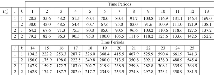
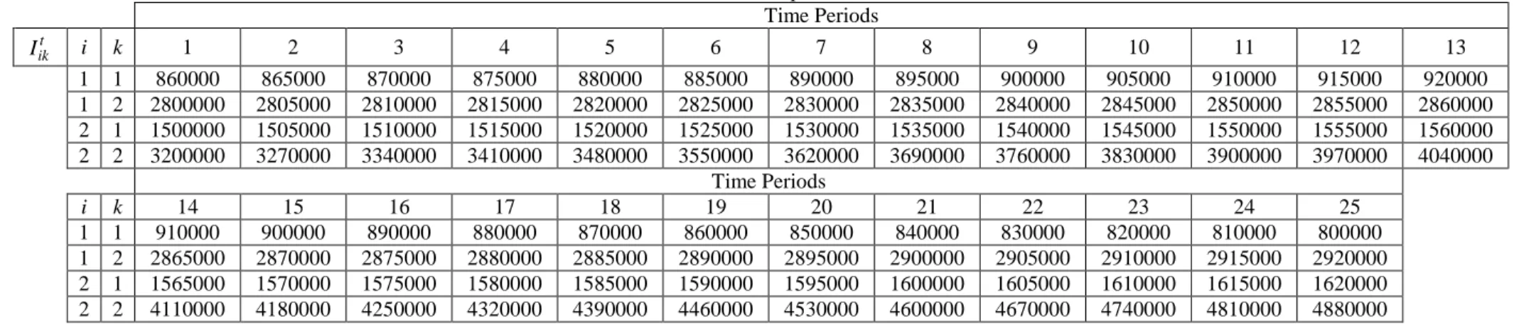
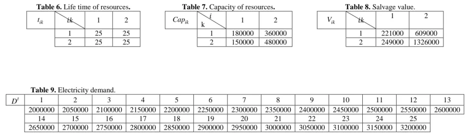
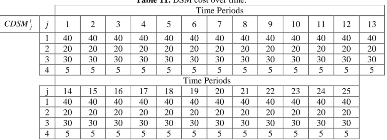
In this subsection, a test problem with two energy technology is considered.Each technology has two different types for four end-uses. Time duration is supposed 25 years and this modelis solved with GAMS 23.2 software. The data related to this problem are shown in the Tables 1-11 are utilized for validation of the proposed model. By supposing this data, Table 12 shows GAMS results in small size.
{1, 2}
i=
,
k={1, 2},
j={1,..., 4}, t ={1, 2,..., 25} and tDSM =10 Table1. Maximum possible saving using DSMj 1 2 3 4
j
P 1000 200 2000 300
Table2. Electricity generation costs. Time Periods t
ik
C i k 1 2 3 4 5 6 7 8 9 10 11 12 13 1 1 88.5 95.6 103.2 111.5 120.4 130.0 140.4 151.7 163.8 176.9 191.1 206.4 229.0 1 2 63.0 68.0 73.5 79.4 85.7 92.6 100.0 108.0 116.6 125.9 136.0 146.9 163.1 2 1 34.2 37.6 41.3 45.5 50.0 55.0 60.5 66.6 73.2 80.6 88.6 97.5 107.2 2 2 34.2 37.6 41.3 45.5 50.0 55.0 60.5 66.6 73.2 80.6 88.6 97.5 107.2
Time Periods
i k 14 15 16 17 18 19 20 21 22 23 24 25 1 1 254.2 282.2 313.3 347.7 386.0 428.4 475.5 527.9 585.9 650.4 721.9 801.3 1 2 181.0 200.9 223.0 247.5 274.8 305.0 338.5 375.8 417.1 463.0 513.9 570.4 2 1 117.9 129.7 142.7 157.0 172.7 189.9 208.9 229.8 252.8 278.1 305.9 336.5 2 2 117.9 129.7 142.7 157.0 172.7 189.9 208.9 229.8 252.8 278.1 305.9 336.5
Table 3. Maintenance costs. Time Periods
't
ik
C i k 1 2 3 4 5 6 7 8 9 10 11 12 13 1 1 28.5 35.6 43.2 51.5 60.4 70.0 80.4 91.7 103.8 116.9 131.1 146.4 169.0 1 2 38.0 43.0 48.5 54.4 60.7 67.6 75.0 83.0 91.6 100.9 111.0 121.9 138.1 2 1 64.2 67.6 71.3 75.5 80.0 85.0 90.5 96.6 103.2 110.6 118.6 127.5 137.2 2 2 79.2 82.6 86.3 90.5 95.0 100.0 105.5 111.6 118.2 125.6 133.6 142.5 152.2
Time Periods
i k 14 15 16 17 18 19 20 21 22 23 24 25 1 1 194.2 222.2 253.3 287.7 326.0 368.4 415.5 467.9 525.9 590.4 661.9 741.3 1 2 156.0 175.9 198.0 222.5 249.8 280.0 313.5 350.8 392.1 438.0 488.9 545.4 2 1 147.9 159.7 172.7 187.0 202.7 219.9 238.9 259.8 282.8 308.1 335.9 366.5 2 2 162.9 174.7 187.7 202.0 217.7 234.9 253.9 274.8 297.8 323.1 350.9 381.5
Table 4. Salvage revenue subtracted from initial value of resource.
Time Periods t
ik
CV i k 1 2 3 4 5 6 7 8 9 10 11 12 13
1 1 100000 100000 100000 100000 100000 100000 100000 100000 100000 100000 100000 100000 100000 1 2 120000 120000 120000 120000 120000 120000 120000 120000 120000 120000 120000 120000 120000 2 1 140000 140000 140000 140000 140000 140000 140000 140000 140000 140000 140000 140000 140000 2 2 170000 170000 170000 170000 170000 170000 170000 170000 170000 170000 170000 170000 170000
Time Periods
i k 14 15 16 17 18 19 20 21 22 23 24 25
1 1 100000 100000 100000 100000 100000 100000 100000 100000 100000 100000 100000 100000 1 2 120000 120000 120000 120000 120000 120000 120000 120000 120000 120000 120000 120000 2 1 140000 140000 140000 140000 140000 140000 140000 140000 140000 140000 140000 140000 2 2 170000 170000 170000 170000 170000 170000 170000 170000 170000 170000 170000 170000
Table 5. Implementation costs.
Time Periods t
ik
I i k 1 2 3 4 5 6 7 8 9 10 11 12 13
1 1 860000 865000 870000 875000 880000 885000 890000 895000 900000 905000 910000 915000 920000 1 2 2800000 2805000 2810000 2815000 2820000 2825000 2830000 2835000 2840000 2845000 2850000 2855000 2860000 2 1 1500000 1505000 1510000 1515000 1520000 1525000 1530000 1535000 1540000 1545000 1550000 1555000 1560000 2 2 3200000 3270000 3340000 3410000 3480000 3550000 3620000 3690000 3760000 3830000 3900000 3970000 4040000
Time Periods
i k 14 15 16 17 18 19 20 21 22 23 24 25
1 1 910000 900000 890000 880000 870000 860000 850000 840000 830000 820000 810000 800000 1 2 2865000 2870000 2875000 2880000 2885000 2890000 2895000 2900000 2905000 2910000 2915000 2920000 2 1 1565000 1570000 1575000 1580000 1585000 1590000 1595000 1600000 1605000 1610000 1615000 1620000 2 2 4110000 4180000 4250000 4320000 4390000 4460000 4530000 4600000 4670000 4740000 4810000 4880000
Table 6. Life time of resources. Table 7. Capacity of resources. Table 8. Salvage value.
ik
t k 1 2 Cap ik
k 1 2 V ik k
1 2
1 25 25 1 180000 360000 1 221000 609000
2 25 25 2 150000 480000 2 249000 1326000
Table 9. Electricity demand.
t
D 1 2 3 4 5 6 7 8 9 10 11 12 13
2000000 2050000 2100000 2150000 2200000 2250000 2300000 2350000 2400000 2450000 2500000 2550000 2600000
14 15 16 17 18 19 20 21 22 23 24 25
2650000 2700000 2750000 2800000 2850000 2900000 2950000 3000000 3050000 3100000 3150000 3200000
Table 10. DSM implementation cost.
t
IDSM 1 2 3 4 5 6 7 8 9 10 11 12 13 14 15 16 17 18 19 20 21 22 23 24 25
1
Table 11. DSM cost over time. Time Periods t
j
CDSM j 1 2 3 4 5 6 7 8 9 10 11 12 13 1 40 40 40 40 40 40 40 40 40 40 40 40 40 2 20 20 20 20 20 20 20 20 20 20 20 20 20 3 30 30 30 30 30 30 30 30 30 30 30 30 30
4 5 5 5 5 5 5 5 5 5 5 5 5 5
Time Periods
j 14 15 16 17 18 19 20 21 22 23 24 25 1 40 40 40 40 40 40 40 40 40 40 40 40 2 20 20 20 20 20 20 20 20 20 20 20 20 3 30 30 30 30 30 30 30 30 30 30 30 30
4 5 5 5 5 5 5 5 5 5 5 5 5
Table 12. GAMS results (Small size)
The aim of illustrating this example is twofold. First, the model is mathematically validated and its feasibility is proven. Secondly, it is indicated that the model is really complex and very time consuming even for such a small test problem. In this case which has only two energy technologies, two different capacities for each technology and 25 years as total number of periods, it takes nearly 2 hours CPU time to find the optimum solution using GAMS optimization solver.One way to accomplish this task in shorter running time is to use of metaheuristic algorithms. The most salient feature of these algorithms that have made them popular among researchers and practitioners is their abilities at providing well-qualified solutions in a very short period of time. A well-known metaheuristic algorithm is GA that tries to find global optimum solution through an evolutionary mechanism. Since, this method is very easy to apply and also very efficient in almost every optimization problems, it is chosen to solve the proposed model for this article. The way that this method is applied for the proposed model is completely discussed in the next section.
4- Solution methodology
Recently, GAs have received considerable attention to be used as an optimization technique to solve the problems in so many fields of science. GA is an intelligent probabilistic search algorithm that works by preserving and adapting the characteristics of a set of trial solutions (npop) over a number of iterations (maxit). Each individual solution is represented by a string which is referred to as chromosome and includes a set of random numbers called genes. GA is capable of retaining desirable characteristics that may be ignored by completely random searches, and this is a good property for an optimization algorithm. Interested readers about the methodology of GA can refer to Rabbani et al. (2016). GA has three general steps as follows:
(1) Generate initial population. (Chromosomes of first population) (2) Calculate fitness function of each chromosome.
(3) New population generation. NO.
Problems CPU times
(second)
Objective function values Number of facilities/kind Time periods
2
Each chromosome includes genes that are binary matrix and these matrices show which facilities are located. There are several ways to code all the stages of GA. The applied GA in this paper is described in next sections.
4-1- Initialization
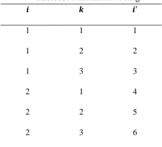
In this problem, the population size is set to be 100. Initially, a random integer matrix that each cell stands for the number of powerhouse type or in period is generated for the first population, and then we utilize a calculating function on each chromosome of the initial population. We have three indices, so primary matrix is three-dimensional matrix, but for convenience, indices and combined together as follows (Table 13):
Table13. Dimension coding
1 1 1
1 2 2
1 3 3
2 1 4
2 2 5
2 3 6
With these new coded indices all of our three-dimensional matrices have been converted to two-dimensional matrices. Therefore, we can show number of powerhouse kind established in period ( ), with the upper part of the following matrix which is shown in Fig 1:
Fig. 1: The structure of first part of chromosome
The lower part of this matrix showsthe amount of SDSMs in each periods.Given the matrix above as an encoded feasible solution, a one-to-one relation between the solution space and the new encoded space can be established. By having this matrix and using a sign function on the first part of the matrix, the value of variable Y can be calculated. Subsequently, variables x, F, and can also be calculated and thus the fitness of each solution is gained.
3
After all of those evaluations, the fitness function is calculated for the population. According to the objective function, the mathematical evaluation wrote in MATLAB software. All chromosomes should fallow up this terms; first, supplying energy demand in every period, second, confirming that we cannot run DSM program in life cycle of another before. For fitness function of any chromosome that cannot supply these terms, a specific penalty policy is considered.In each period, it is consideredthat if its demand is not supplied, it will charge 1,000,000$ cost penalty and each demand side management that began in other DSM life time will charge 2,000,000$ cost penalty. 4-3- Crossover operator
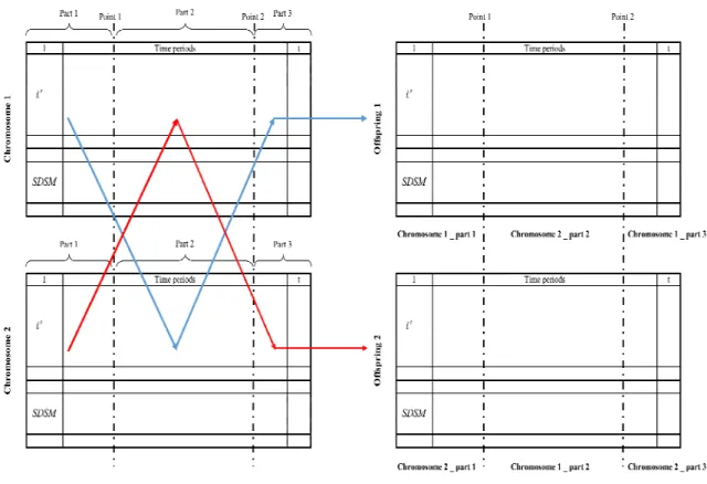
For parent selection, tournament method is selected. In this method, specific number chromosomes are selected randomly and the best chromosome is the tournament winner. Two crossover operators are applied randomly for the optimization. First one is column two points; second one is row one point, one time for powerhouse and another one for SDSMs (Fig 2). These are formal crossovers, but for earlier convergence the local search is decided to run.
Fig. 2: Method of creating crossovers
4-4- Mutation
Two different mutation operators are applied for the GA used to optimize the problem. The first one changes randomly in the first period of matrix (Fig 3); the second one changes in some of cells except the first period of chromosomes (Fig 4). Number of mutations in is equal with rate of mutation (Mu) × number of cells in every chromosome.
4
Fig. 3: First method for creating mutation
4-5- Local search
Two different local search functions are applied. In the first one, some chromosomes are selected, then with a random function we subtract 1 or 2 or sum 1 with chosen sells (Fig 5). In the second function, we calculate sum of generating potential of setting up powerhouses and then if this sum was more than demand of that period, we reduce the number of powerhouses in that period (Fig 6). In the first local search, we look for a chromosome that is very close to the original chromosome but we hope of some change, the fitness function become well. In the second local search, we hope to reduce the cost with decreasing the number of powerhouses set up in every period.
5
Fig. 6: Local search No.2 algorithm
4-6- Replacement strategy
The elitist strategy is applied in this problem. In each iteration the best chromosome selected as one of the chromosomes in the next population, in addition to the chromosomes (parents and off springs) which are ranked after cross over and mutation according to their objective values. Among these ranked chromosomes, 100 of the best chromosomes are selected as the next population.
5- Experimental results
This section is mainly focused on indicating how well the proposed genetic algorithm performs. To do so, a small size problem is firstly solved by both GAMS software and GA, and then the obtained results are compared. Afterward, through setting up nine different problems of different size the performance of GA is shown for problems of larger sizes. The outcomes have been demonstrated in Tables 14 and 15.
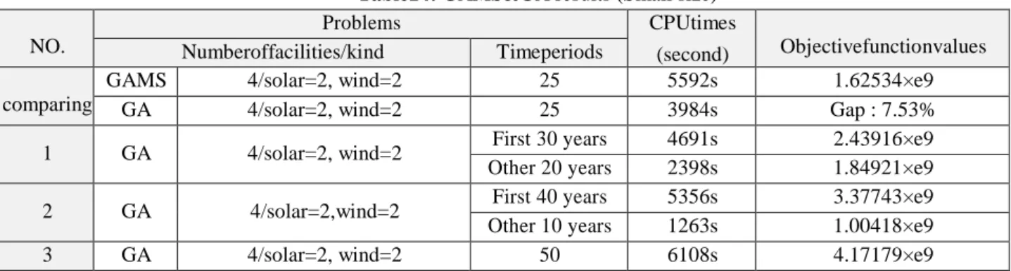
Table14: GAMS&GA results (Small size) NO.
Problems CPUtimes
(second) Objectivefunctionvalues Numberoffacilities/kind Timeperiods
comparing
GAMS 4/solar=2, wind=2 25 5592s 1.62534×e9
GA 4/solar=2, wind=2 25 3984s Gap : 7.53%
1 GA 4/solar=2, wind=2 First 30 years 4691s 2.43916×e9 Other 20 years 2398s 1.84921×e9 2 GA 4/solar=2,wind=2 First 40 years 5356s 3.37743×e9
Other 10 years 1263s 1.00418×e9
6
Table15: GA results (Large size)
NO.
Problems CPUtimes
(second) Objectivefunctionvalues Numberoffacilities/kind Timeperiods
4 6/solar=2, wind=2, hybrid=1, geo=1
First 30 years 6048s 2.51914×e9 Other 20 years 4309s 1.89132×e9
5 6/solar=2,wind=2, hybrid=1, geo=1
First 40 years 6652s 3.45474×e9 Other 10 years 2201s 1.10429×e9 6 6/solar=2, wind=2, hybrid=1, geo=1 50 7689s 4.27527×e9
7 8/solar=3, wind=2, hybrid=2, geo=1
First 30 years 8114s 2.31347×e9 Other 20 years 5319s 1.95721×e9
8 8/solar=3, wind=2, hybrid=2, geo=1
First 40 years 8513s 3.09975×e9 Other 10 years 3914s 1.24781×e9 9 8/solar=3, wind=2,hybrid=2, geo=1 50 10449s 4.06216×e9
As it can be seen from Tables 14 and 15, the total number of periods has been considered to be 50 years, while 9 different problems and 3 scenarios are investigated. In the first scenario, the energy supply plan was initially determined for the first 30 years and then for the next 20 years; in the second scenario, the energy plan of the first 40 years was established at the outset and after that the next 10 years’ energy plan was investigated. At last, in the third scenario, all the 50 years was taken into account altogether. The obtained results indicate that when the time period is considered as one big period of time, the outcomes are more effective and practical than those obtained when the whole period of time is divided into small bucket periods.
This superiority for big bucket plans is not only related to achieving cost-effective plans but also contributes to reaching shorter CPU times for solving the problems. Therefore, it can be concluded that life cycle analysis is a crucial tool for making energy planning decisions.
Moreover, it can be deduced that the length of planning period is a key factor in selecting the appropriate type of energy resource technology. For instance, for time periods less than 35 years, the use of hydro power plants is not recommended. It is mostly due to the fact that the usual life cycle of a typical hydro power plant is about 50 years and thus for planning periods shorter than 50 years hydro power plants are not a cost-effective solution.
6- Conclusions and future directions
The main aim of this paper was to select the best portfolio of renewable energy technologies (RETs) for electrifying a secluded area. Minimizing total costs of the system was considered as the key feature in finding the optimum decision. In order to make the optimum plan more realized, the technique of life cycle analysis was applied. To cope with the problem a nonlinear mixed integer programming formulation was developed. Also, a genetic algorithm was proposed to solve the formulation for large scale test problems. Afterward a variety of test problems in three different scenarios was considered. The obtained results indicated that when the time period is considered as one big period of time, the outcomes are more effective and practical than those obtained when the whole period of time is divided into small bucket periods. This superiority for big bucket plans is not only related to achieving
7
cost-effective plans, but also contributes to reaching shorter CPU times for solving the problems. Therefore, it is concluded that life cycle analysis is a crucial tool for making energy planning decisions.Moreover, it was shown that the length of planning period is a key factor in selecting the appropriate type of energy resource technology. For instance, for time periods less than 35 years, the use of hydro power plants is not recommended. It is mostly due to the fact that the usual life cycle of a typical hydro power plant is about 50 years and thus for planning periods shorter than 50 years hydro power plants are not a cost-effective solution.
For future study, the respected researchers are advised to add environmental factors to the decision criteria and reformulate the model accordingly. Also, skillful human resource availability should be investigated in such secluded areas.
References:
Bhat, I. K., & Prakash, R. (2009). LCA of renewable energy for electricity generation systems—A review. Renewable and Sustainable Energy Reviews,13(5), 1067-1073.
Chang, Y., Ries, R. J., & Wang, Y. (2010). The embodied energy and environmental emissions of construction projects in China: an economic input–output LCA model. Energy
Policy, 38(11), 6597-6603.
Cooper, J. M., Butler, G., &Leifert, C. (2011). Life cycle analysis of greenhouse gas emissions from organic and conventional food production systems, with and without bio-energy options. Njas-Wageningen Journal of Life Sciences, 58(3), 185-192.
Crawford, R. H. (2009). Life cycle energy and greenhouse emissions analysis of wind turbines and the effect of size on energy yield. Renewable and Sustainable Energy Reviews, 13(9), 2653-2660.
Devadas, V. (2001). Planning for rural energy system: part I. Renewable and Sustainable
Energy Reviews, 5(3), 203-226.
Dismukes, J. P., Miller, L. K., &Bers, J. A. (2009). The industrial life cycle of wind energy electrical power generation: ARI methodology modeling of life cycle dynamics. Technological
Forecasting and Social Change, 76(1), 178-191.
Dones, R., &Frischknecht, R. (1998). Life‐cycle assessment of photovoltaic systems: results of Swiss studies on energy chains. Progress in Photovoltaics: Research and Applications, 6(2), 117-125.
Fay, R., Treloar, G., &Iyer-Raniga, U. (2000). Life-cycle energy analysis of buildings: a case study. Building Research & Information, 28(1), 31-41.
Frick, S., Kaltschmitt, M., &Schröder, G. (2010). Life cycle assessment of geothermal binary power plants using enhanced low-temperature reservoirs.Energy, 35(5), 2281-2294.
Góralczyk, M. (2003). Life-cycle assessment in the renewable energy sector.Applied
Energy, 75(3), 205-211.
Heller, M. C., Keoleian, G. A., Mann, M. K., & Volk, T. A. (2004). Life cycle energy and environmental benefits of generating electricity from willow biomass.Renewable Energy, 29(7), 1023-1042.
Herran, D. S., & Nakata, T. (2008). Renewable technologies for rural electrification in Colombia: a multiple objective approach. International Journal of Energy Sector
8
Hertwich, E. G. (2005). Life cycle approaches to sustainable consumption: a critical review. Environmental science & technology, 39(13), 4673-4684.
Hiremath, R. B., Kumar, B., Deepak, P., Balachandra, P., Ravindranath, N. H., &Raghunandan, B. N. (2009). Decentralized energy planning through a case study of a typical village in India. Journal of renewable and sustainable energy,1(4), 043103.
Iniyan, S., Suganthi, L., &Jagadeesan, T. R. (1998). Renewable energy planning for India in 21st century. Renewable energy, 14(1), 453-457.
Jorquera, O., Kiperstok, A., Sales, E. A., Embiruçu, M., &Ghirardi, M. L. (2010). Comparative energy life-cycle analyses of microalgal biomass production in open ponds and photobioreactors. Bioresource technology, 101(4), 1406-1413.
Kazemi, S. M., & Rabbani, M. (2013). An integrated decentralized energy planning model considering demand-side management and environmental measures. Journal of Energy, 2013. Martinez, E., Sanz, F., Pellegrini, S., Jimenez, E., & Blanco, J. (2009). Life cycle assessment of a multi-megawatt wind turbine. Renewable Energy, 34(3), 667-673.
Mullally, H. (2007). Applying the California evaluation criteria to Nova Scotia's demand-side
management programs. ProQuest.
Moura, P. S., & de Almeida, A. T. (2010). Multi-objective optimization of a mixed renewable system with demand-side management. Renewable and Sustainable Energy Reviews, 14(5), 1461-1468.
Pelzer, R., Mathews, E. H., Le Roux, D. F., &Kleingeld, M. (2008). A new approach to ensure successful implementation of sustainable demand side management (DSM) in South African mines. Energy, 33(8), 1254-1263.
Pehnt, M. (2006). Dynamic life cycle assessment (LCA) of renewable energy technologies. Renewable energy, 31(1), 55-71.
Rabbani, M., Farrokhi-asl, H., & Rafiei, H. (2016). A hybrid genetic algorithm for waste collection problem by heterogeneous fleet of vehicles with multiple separated compartments. Journal of Intelligent & Fuzzy Systems, 30(3), 1817-1830.
Rodríguez, R., Ruyck, J. D., Díaz, P. R., Verma, V. K., & Bram, S. (2011). An LCA based indicator for evaluation of alternative energy routes. Applied Energy,88(3), 630-635.
Schleisner, L. (2000). Life cycle assessment of a wind farm and related externalities. Renewable
energy, 20(3), 279-288.
Senjyu, T., Hayashi, D., Yona, A., Urasaki, N., & Funabashi, T. (2007). Optimal configuration of power generating systems in isolated island with renewable energy. Renewable
Energy, 32(11), 1917-1933.
Sherwani, A. F., &Usmani, J. A. (2010). Life cycle assessment of solar PV based electricity generation systems: A review. Renewable and Sustainable Energy Reviews, 14(1), 540-544. Tonini, D., &Astrup, T. (2012). LCA of biomass-based energy systems: a case study for Denmark. Applied Energy, 99, 234-246.
Weisser, D. (2007). A guide to life-cycle greenhouse gas (GHG) emissions from electric supply technologies. Energy, 32(9), 1543-1559.