Journal of Industrial and Systems Engineering Vol. 8, No. 2, pp 13-30
Spring 2015
A new mathematical model for intensity matrix
decomposition using multileaf collimator
Vahid Mahmoodian1*, Ahmad Makui2, Mohammad Reza Gholamian3
1,2,3 Department of Industrial Engineering, Iran University of Science and
Technology, Narmak, , Tehran, Iran
[email protected], [email protected], [email protected]
Abstract
Cancer is one of the major causes of death all over the globe and radiotherapy is considered as one of its most effective treatment methods. Designing a radiotherapy treatment plan was done entirely manually in the past. Recently, Intensity Modulated Radiation Therapy (IMRT) was introduced as a new technology with advanced medical equipment in the recent years. IMRT provides the opportunity to deliver complex dose distributions to cancer cells while sparing the vital tissues and cells from the harmful effects of radiations. Designing an IMRT treatment plan is a very complex matter due to the numerous calculations and parameters which must be decided for. Such treatment plan is designed in three separate phases: 1) selecting the number and the angle of the beams, 2) extracting the intensity matrix or the corresponding dose map of each beam, and 3) realizing each intensity matrix. The third phase has been studied in this research and a nonlinear mathematical model has been proposed for multileaf collimators. The proposed model has been linearized through two methods and an algorithm has been developed on its basis in order to solve the model with cardinality objective function. Obtained results are then compared with similar studies in the literature which reveals the capability of proposed method.
Keywords: Intensity modulated radiation therapy (IMRT), Decomposing intensity matrix, Multileaf collimator, Benders decomposition, Integer programming.
1*Corresponding author
ISSN: 1735-8272, Copyright c 2015 JISE. All rights reserved
1. Introduction
Cancer is one of the most common diseases among the world and one of the most effective cures for it is radio therapy(Taşkın and Cevik, 2013). Designing a treatment plan was done completely manually in the past but a little more than ten years ago, as technology and medical equipment advanced,intensity modulated radiation therapy (IMRT) was introduced and the results of using it indicated its significant effects on the dose that the cancer cells received while the vital and natural tissues were being spared(Meyer et al., 2006). This was due to the fact that it had a greater potential in comparison with the other methods regarding proportionality of dose distribution with the target mass. However, it increased the number of treatment options and parameters (which had to be decided) so much such that it caused manual and wholesome designing of a treatment plan impossible; since there were numerous calculations to be done. Therefore one such treatment planning is done in three different phases: 1) selecting the number and the angle of the beams, 2) extracting the intensity pattern or the corresponding dose map of each beam, and 3) realizing each intensity matrix. The reader can refer to works done byEhrgott et al. (2008) and Schlegel and Mahr (2007) in order to obtain more information.
The third phase problem (i.e. realization problem) includes decomposing the intensity matrix obtained from phases one and two to matrix shapes or segments which can be formed in radiation therapy machines. The aim of the realization or segmentation problem, in general, is to minimize the treatment time due to the risk of involuntary movements of the patient, making him or her more comfortable, and also efficient use of the equipments along treatment. Multileaf collimators (MLC) are the main instruments for realization of intensity matrix radiation therapy machines which have been used in IMRT since 1996 (Meyer et al., 2006). MLC is an instrument with mobile paired metal leaves within grooves which prevents beams outside the dose area from reaching the body.
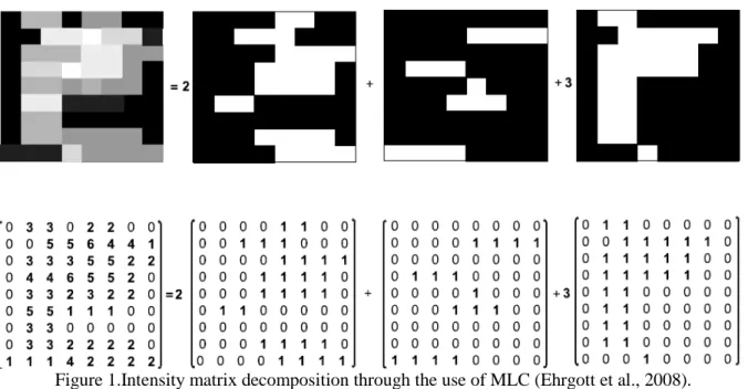
The issue that makes the intensity matrix decomposition difficult, is the physical limitations related to collimators in producing shape matrixes. For instance, the distance between the two opposing leaves remains open in each line in MLCs. In Figure 1 for example realization of one matrix has been done through breaking it down into three matrixes which the black areas in three squares correspond to the left and right leaves of MLC. The beams pass through the open areas between the leaves (perpendicular to the sheet of segments). It should be noted that the dose area is divided into small parts called bixel as shown in Figure 1.
Figure 1.Intensity matrix decomposition through the use of MLC (Ehrgott et al., 2008).
Using modern treatment planning algorithms in IMRT from 2002 to 2005,the planning time has decreased from 4 hours to 2 hours and the treatment time (executing the treatment plan) by four times in average (Meyer et al., 2006). This was due to the fact that the average number of essential segments for realizing intensity matrixes decreased by approximately 50% for instance (Meyer et al., 2006).
Decomposing the intensity matrix has been presented in the literature with three major objectives: 1) Beam On Time (BOT), 2) Decomposition Cardinality (DC), and 3) a combination of the two aforementioned objectives called Total Treatment Time (TTT). Numerous researches have been carried out on the first objective function (Ahuja and Hamacher, 2005, Siochi, 1999, Engel, 2005) and efficient algorithms have been presented for them even in cases containing additional physical constraints(Boland et al., 2004). In contrast, proposing an efficient algorithm which can optimally solve the intensity matrix decomposition problems with the least number of segments (i.e. cardinality objective function) is a difficult matter. So that it is strictly NP-hard even for matrixes with only one row or one column (Baatar et al., 2005, Collins et al., 2007). This objective function aims at minimizing the number of essential segments for realization of the intensity matrix.
Baatar et al. (2005)indicated that the DC problem can be solved in polynomial time only under conditions where the intensity matrix is an integer coefficient of a binary matrix. Therefore the initial studies aimed at minimizing cardinality among solutions with the best beam on time (Engel, 2005, Kalinowski, 2009). However later finding the optimal solution of these problems gained more importance.
Mak(2007) used integer programming to accurately solve the DC problem which included many variables and this made it difficult to solve for real size data. Baatar et al. (2007) also developed a model known as Counter Model for solving beam on time and decomposition cardinality problems lexicographically. The model has been analyzed by Cambazard et al. (2010) later. They modeled the decomposing the intensity matrix to binary matrixes with consecutive-ones (C1) property through turning it into the shortest path problem. They solved their model by using column generation and Dantzing-Wolfe decomposition methods and showed that it was more efficient in comparison with the algorithms proposed by Taskin et al. (2010).
An exact algorithm has recently been introduced by Ernst et al. (2009) which researched for a feasible sequence for all rows of the matrix through generating Monitor Unit (MU) sequences heuristically. This algorithm would start with an initial solution and would gradually decrease the segments. This algorithm became a major inspiration for other algorithms which considered the total treatment time as well as cardinality objective function. Taskin et al. (2010)considered the objective function of TTT problem as a weighted sum of beam on time and decomposition cardinality and developed a decomposition algorithm which was compatible with cardinality objective functions and total treatment time under the influence of Ernst et al.’s (Ernst et al., 2009)algorithm. They generated a set of candidate MU values each of which could be dedicated to one segment. This series was named allowable intensity multi set and if there is decomposition for a row in a subset of that allowable MU values set, that would be a compatible MU sequence with that row. It is obvious that if the values of an allowable intensity multi set are compatible with all the rows of a matrix, they would be a feasible set. They claimed for the first time that they have presented an exact algorithm for solving problems with practical dimension through a combination of integer programming and combinatorial search techniques. They reported the results obtained from application of their algorithm on 25 real clinical data and also 100 random data. Mason et al. (2012)eventually generalized Ernst et al.’s work to the TTT problem. They proposed a similar algorithm which searched for a feasible sequence for all the rows of the matrix through starting with a heuristically initial solution such as TNMU-NS(Engel, 2005) and generating MU sequences based on that solution.
In this paper, a nonlinear mathematical model has been proposed in order to decompose an intensity matrix through multileaf collimators with two DC and TTT objective functions. This model has been linearized through two approaches and an algorithm has been developed based on them for the purposes of solving the problem with the cardinality objective function and the obtained results have been compared with similar studies in the literature.
The rest of the paper is organized as follows. The model and its linearization procedure have been described in section 2. Solving method presented for DC objective function has been explained in section 3 and numerical results is analyzed in section 4. Conclusions and suggestions for future researches are presented in section 5.
2. Model Description
2.1. The mathematical model
The presented model is explained as below: Sets:
𝑖𝑖 The set of rows of the intensity matrix or dose map;𝑖𝑖= 1, … ,𝑀𝑀
𝑗𝑗 The set of columns of the intensity matrix or dose map;𝑗𝑗 = 1, … ,𝑁𝑁
𝑠𝑠 The set of segments;𝑠𝑠= 1, … ,𝑆𝑆 Parameters:
𝑎𝑎𝑖𝑖𝑖𝑖 prescribed dose to bixel(𝑖𝑖,𝑗𝑗)
Variables:
𝑥𝑥𝑖𝑖𝑖𝑖𝑖𝑖 1 if the bixel (𝑖𝑖,𝑗𝑗) is open in segment 𝑠𝑠 and 0 otherwise, 𝑦𝑦𝑖𝑖 1 if segment 𝑠𝑠 is used and 0 otherwise,
𝑙𝑙𝑖𝑖𝑖𝑖𝑖𝑖 1 if the 𝑖𝑖th left leaf covers up to column 𝑗𝑗 in segment 𝑠𝑠 and 0 otherwise, 𝑟𝑟𝑖𝑖𝑖𝑖𝑖𝑖 1 if the 𝑖𝑖th right leaf covers up to column 𝑗𝑗 in segment 𝑠𝑠 and 0 otherwise,
𝑏𝑏𝑖𝑖 Weight of segment 𝑠𝑠
Mathematical model:
(1)
𝑀𝑀𝑖𝑖𝑀𝑀 � 𝑦𝑦𝑖𝑖 𝑖𝑖
(2)
∀𝑖𝑖,𝑗𝑗 𝑠𝑠.𝑡𝑡 � 𝑏𝑏𝑖𝑖𝑥𝑥𝑖𝑖𝑖𝑖𝑖𝑖
𝑖𝑖
= 𝑎𝑎𝑖𝑖𝑖𝑖
(3)
∀𝑖𝑖,𝑗𝑗,𝑠𝑠 𝑙𝑙𝑖𝑖𝑖𝑖𝑖𝑖+𝑟𝑟𝑖𝑖𝑖𝑖𝑖𝑖+𝑥𝑥𝑖𝑖𝑖𝑖𝑖𝑖 = 1
(4)
∀𝑖𝑖,𝑗𝑗 <𝑀𝑀,𝑠𝑠 𝑙𝑙𝑖𝑖,𝑖𝑖+1,𝑖𝑖 ≤ 𝑙𝑙𝑖𝑖,𝑖𝑖,𝑖𝑖
(5)
∀𝑖𝑖,𝑗𝑗 <𝑀𝑀,𝑠𝑠 𝑟𝑟𝑖𝑖𝑖𝑖𝑖𝑖 ≤ 𝑟𝑟𝑖𝑖,𝑖𝑖+1,𝑖𝑖
(6)
∀𝑠𝑠, � � 𝑥𝑥𝑖𝑖𝑖𝑖𝑖𝑖
𝑖𝑖 𝑖𝑖
≤ 𝑀𝑀𝑁𝑁𝑦𝑦𝑖𝑖
(7)
∀𝑖𝑖,𝑗𝑗,𝑠𝑠 𝑏𝑏𝑖𝑖 ≥ 0,𝑥𝑥𝑖𝑖𝑖𝑖𝑖𝑖,𝑦𝑦𝑖𝑖,𝑙𝑙𝑖𝑖𝑖𝑖𝑖𝑖,𝑟𝑟𝑖𝑖𝑖𝑖𝑖𝑖 ∈{0, 1}
Equation (1) indicates the cardinality objective function and constraint (2) which is the only nonlinear expression of the model guarantees the realization of prescribed dose. Constraints (3-5) simulate the collimator’s leafs and guarantee C1 property in each row of the segments and constraint (6) counts the number of segments. The total number of nonzero elements of the intensity matrix can replace 𝑀𝑀×𝑁𝑁term which is equal to the total number of the bixels of the intensity matrix in order to tighten solution space.
The total treatment time objective function has been considered mostly as a weight combination of setup time and the beam on time assuming a constant time for setup of each segment, in the literature(Taşkın et al., 2012, Mason et al., 2012, Cambazard et al., 2012). Here the total treatment time objective function can be written as follows with the same assumption:
(8)
𝑀𝑀𝑖𝑖𝑀𝑀 𝑤𝑤1� 𝑦𝑦𝑖𝑖 𝑖𝑖
+𝑤𝑤2� 𝑏𝑏𝑖𝑖 𝑖𝑖
Where𝑤𝑤1represents each segment’s setup time and 𝑤𝑤2 is an amount of time which is needed to deliver one monitor unit.
2.2. Mathematical model linearization
The above mentioned model can be linearized through adding a subscript which indicates the amount of monitor unit of each segment. This type of linearization guarantees the integrality of beam on time values but increases the number of variables exponentially. Therefore determining
a good upper bound for the monitor units can significantly increase its efficiency. The largest element of the intensity matrix (𝑎𝑎𝑚𝑚𝑚𝑚𝑚𝑚 = max
𝑖𝑖,𝑖𝑖 �𝑎𝑎𝑖𝑖𝑖𝑖�) is an obvious bound for the monitor units of
the segments. The linearized model is presented as below: Sets:
𝑏𝑏 Set of weights 𝑏𝑏= 1, … ,𝐵𝐵 Variables:
𝑥𝑥𝑖𝑖𝑖𝑖𝑖𝑖𝑖𝑖 1 if the bixel(𝑖𝑖,𝑗𝑗) is open in segment 𝑠𝑠 with beam on time amount 𝑏𝑏,and 0
otherwise,
𝑦𝑦𝑖𝑖𝑖𝑖 1 if segment 𝑠𝑠 with its beam on time amount equals to𝑏𝑏 is used, and 0 otherwise, 𝑙𝑙𝑖𝑖𝑖𝑖𝑖𝑖 1 if the 𝑖𝑖th left leaf covers segment 𝑠𝑠 up to column 𝑗𝑗, and 0 otherwise,
𝑟𝑟𝑖𝑖𝑖𝑖𝑖𝑖 1 if the 𝑖𝑖th right leaf covers segment 𝑠𝑠 up to column 𝑗𝑗, and 0 otherwise
Mathematical model:
(9)
𝑀𝑀𝑖𝑖𝑀𝑀 � � 𝑦𝑦𝑖𝑖𝑖𝑖 𝑖𝑖 𝑖𝑖
(10)
∀𝑖𝑖,𝑗𝑗 𝑠𝑠.𝑡𝑡 � � 𝑏𝑏𝑥𝑥𝑖𝑖𝑖𝑖𝑖𝑖𝑖𝑖
𝑖𝑖 𝑖𝑖
=𝑎𝑎𝑖𝑖𝑖𝑖
(11)
∀𝑖𝑖,𝑗𝑗,𝑠𝑠 𝑙𝑙𝑖𝑖𝑖𝑖𝑖𝑖+𝑟𝑟𝑖𝑖𝑖𝑖𝑖𝑖+� 𝑥𝑥𝑖𝑖𝑖𝑖𝑖𝑖𝑖𝑖
𝑖𝑖
= 1
(12)
∀𝑖𝑖,𝑗𝑗 <𝑁𝑁,𝑠𝑠 𝑙𝑙𝑖𝑖,𝑖𝑖+1,𝑖𝑖 ≤ 𝑙𝑙𝑖𝑖,𝑖𝑖,𝑖𝑖
(13)
∀𝑖𝑖,𝑗𝑗 <𝑁𝑁,𝑠𝑠 𝑟𝑟𝑖𝑖𝑖𝑖𝑖𝑖≤ 𝑟𝑟𝑖𝑖,𝑖𝑖+1,𝑖𝑖
(14)
∀𝑠𝑠,𝑏𝑏 � � 𝑥𝑥𝑖𝑖𝑖𝑖𝑖𝑖𝑖𝑖
𝑖𝑖 𝑖𝑖
≤ 𝑀𝑀𝑁𝑁𝑦𝑦𝑖𝑖𝑖𝑖
(15)
∀𝑠𝑠 � 𝑦𝑦𝑖𝑖𝑖𝑖
𝑖𝑖
≤ 1
(16)
∀𝑖𝑖,𝑗𝑗,𝑠𝑠 𝑥𝑥𝑖𝑖𝑖𝑖𝑖𝑖𝑖𝑖,𝑦𝑦𝑖𝑖𝑖𝑖,𝑙𝑙𝑖𝑖𝑖𝑖𝑖𝑖,𝑟𝑟𝑖𝑖𝑖𝑖𝑖𝑖∈{0, 1}
The objective function and all the constraints have the same corresponding role in both models. The difference is that additive constraint (15) has been added to the linear model. The solution violating this constraint might not be actually infeasible but obviously in the optimal solution each of the segments appears once. This constraint can tighten the feasible space of the model.
On the other hand, the above mentioned nonlinear model can be linearized through another method by changing the variable and adding three constraints. This time we should only define a new positive variable as 𝑧𝑧𝑖𝑖𝑖𝑖𝑖𝑖 =𝑏𝑏𝑖𝑖𝑥𝑥𝑖𝑖𝑖𝑖𝑖𝑖, 𝑖𝑖 ∈{1,2, … ,𝑀𝑀} ,𝑗𝑗 ∈{1, 2, … ,𝑁𝑁} , and 𝑠𝑠 ∈ {1, 2, … ,𝑆𝑆}which is applied with four linear constraints (17- 21) while replacing constraint (2). The variable𝑧𝑧𝑖𝑖𝑖𝑖𝑖𝑖 can be defined as the dose which would be delivered to bixel(𝑖𝑖,𝑗𝑗) in segment 𝑠𝑠.
(17)
∀𝑖𝑖,𝑗𝑗 � 𝑧𝑧𝑖𝑖𝑖𝑖𝑖𝑖
𝑖𝑖
=𝑎𝑎𝑖𝑖𝑖𝑖
(18)
∀𝑖𝑖,𝑗𝑗,𝑠𝑠 𝑧𝑧𝑖𝑖𝑖𝑖𝑖𝑖 ≤ 𝑏𝑏𝑖𝑖
(19)
∀𝑖𝑖,𝑗𝑗,𝑠𝑠 𝑧𝑧𝑖𝑖𝑖𝑖𝑖𝑖+ℳ(1− 𝑥𝑥𝑖𝑖𝑖𝑖𝑖𝑖) ≥ 𝑏𝑏𝑖𝑖
(20)
∀𝑖𝑖,𝑗𝑗,𝑠𝑠 𝑧𝑧𝑖𝑖𝑖𝑖𝑖𝑖≤ ℳ𝑥𝑥𝑖𝑖𝑖𝑖𝑖𝑖
(21)
∀𝑖𝑖,𝑗𝑗,𝑠𝑠 𝑧𝑧𝑖𝑖𝑖𝑖𝑖𝑖 ≥ 0
Where 𝑀𝑀is an enough positive large number in constraints (19) and (20) and can be replaced by 𝛼𝛼𝑚𝑚𝑚𝑚𝑚𝑚. However it is clear that setting the smaller value to this number, can caused the solution space to be tightened(Taşkın et al., 2012). Constraints (18) and (19) guarantee that if bixel(𝑖𝑖,𝑗𝑗) is open in segment 𝑠𝑠(𝑥𝑥𝑖𝑖𝑖𝑖𝑖𝑖= 1) a dose equal to 𝑏𝑏𝑖𝑖 will surely pass through it (𝑧𝑧𝑖𝑖𝑖𝑖𝑖𝑖 =
𝑏𝑏𝑖𝑖) and if it is closed (𝑥𝑥𝑖𝑖𝑖𝑖𝑖𝑖= 0) constraint (20) is activated and the passing dose will drop to
zero.
3. The presented solution
The details of the presented algorithm based on the developed model will be explained in this section. The matrix’s rows are first organized based on decreasing order ofTNMU(Engel, 2005) complexity C(A) and the most complex row, 𝑖𝑖* (the first row in rank) will be selected. The minimum decomposition cardinality of each row will be calculated through the Benders’ decomposition method and so the lower bound of the cardinality of the total decomposition of the matrix (𝑘𝑘) will be obtained. Then through limiting the number of segment sets of the presented mathematical model to the lower bound (S:= 𝑘𝑘), the number of the rows to one (𝑀𝑀 = 1), and removing the objective function it would be possible to simultaneously examine the feasibility of the monitor units sequence𝑏𝑏𝑖𝑖,𝑠𝑠 ∈{1, … ,𝑆𝑆}, which are generated through two related methods. In such manner that the sequences of monitor units 𝑏𝑏�𝑖𝑖 are entered as parameter to a linear system of inequalities including (3-5) and the following constraint and its feasibility will be examined for all the rows one by one by tracking the predetermined manner:
(22)
∀𝑖𝑖,𝑗𝑗 � 𝑏𝑏�𝑖𝑖𝑥𝑥𝑖𝑖𝑖𝑖𝑖𝑖
𝑖𝑖
= 𝐼𝐼𝑖𝑖𝑖𝑖
It is obvious that if a given sequence is feasible for all rows, it would be feasible for the entire matrix as well, and therefore a decomposition would be obtained with cardinality𝑆𝑆. Hence the process of generating new monitor unit sequences (𝑏𝑏𝑖𝑖) and increasing the bound of the number of segments must continue until we reach to one such sequence. The methods of generating new monitor unit sequences (𝑏𝑏𝑖𝑖) guarantee the optimality of this process.
Monitor unit sequence generating methods play the main role in this algorithm and have a significant effect on the time needed to reach a feasible answer. The first linearized model has the capability to make taboo the determined sequence𝑇𝑇𝑆𝑆𝑖𝑖 ،𝑠𝑠 ∈{1, … ,𝑆𝑆}for the model through adding a constraint like (56). Which means it prevents the model from reaching these sequences
as asolution. The observations have indicated that the feasible monitor sequences are very similar to one another in such manner that they differ from each other by ±1 unit correspondingly (Mason et al., 2012). Therefore the obtained sequences can be used to generate new sequences. The algorithm will be explained in detail in the following section.
3.1. Solving a single row model through Benders decomposition method
The amount of computation and required memory is one of the important points in modeling and solving optimization problems which increases significantly as the number of variables and constraints increase. Thus the traditional methods which made all the decisions simultaneously through solving an integrated optimization model became inefficient as the variables and constraints increased and they were replaced by multistage algorithms such as Benders decomposition (Benders, 2005, Pishvaee et al., 2014). Unlike the traditional methods these algorithms divide the decision making process into a number of stages. In the first stage of the Benders decomposition, the master problem, which includes a set of variables (mostly integer), is solved and the values of other variables are determined in the second stage through solving the sub-problem. In the sub-problem the values of the master problem variables are substituted as known parameters. Therefore if the sub-problem becomes infeasible with those values, the master problem will be directed toward feasible region of the whole problem through adding one or more cuts which are resulted from the dual of sub-problem. And so a number of small problems will be solved instead of a large problem which is plausible due to the large amount of computational resources needed for solving large problems.
Taking into consideration the fact that it has been shown that the DC problem is NP-hard even for single row matrixes (Baatar et al., 2005), the Benders decomposition approach can aid shortening the time and decreasing the memory needed for solving single row problems. Taskin et al. (2012)used this method to solve their model as well. As mentioned previously we must reach to the minimum cardinality of decomposing each and every row of the matrix in order to obtain the lower bound for entire matrix decomposition cardinality.
Consider linearized model (23-32). This model has been adapted to problems with single row matrixes. A linear model for an𝑀𝑀×𝑁𝑁size intensity matrix and the upper bound (i.e. the number of essential segments for decomposing)𝑆𝑆, has 4𝑀𝑀𝑁𝑁𝑆𝑆+ 2𝑆𝑆 variables and 6𝑀𝑀𝑁𝑁𝑆𝑆+𝑀𝑀𝑁𝑁+ 2𝑆𝑆 constraints. This number decreases by more than 𝑀𝑀 times when it turned into single row state. As a result the conditions are set for solving the problem through Benders decomposition method.
Variables:
1 if bixel(𝑖𝑖,𝑗𝑗) is open in segment s and 0 otherwise,
𝑥𝑥𝑖𝑖𝑖𝑖
Delivered dose to bixel(𝑖𝑖,𝑗𝑗) through segment 𝑠𝑠,
𝑧𝑧𝑖𝑖𝑖𝑖
1 if segment 𝑠𝑠 is used and 0 otherwise,
𝑦𝑦𝑖𝑖
1 if the left leaf in segment 𝑠𝑠 covers up to column 𝑗𝑗 and 0 otherwise,
𝑙𝑙𝑖𝑖𝑖𝑖
1 if the right leaf in segment 𝑠𝑠 covers up to column 𝑗𝑗 and 0 otherwise,
𝑟𝑟𝑖𝑖𝑖𝑖
The monitor unit amount of segment 𝑠𝑠
𝑏𝑏𝑖𝑖
Mathematical model:
(23)
𝑀𝑀𝑖𝑖𝑀𝑀 � 𝑦𝑦𝑖𝑖 𝑖𝑖
(24)
∀𝑗𝑗 𝑠𝑠.𝑡𝑡. � 𝑧𝑧𝑖𝑖𝑖𝑖
𝑖𝑖
=𝑎𝑎𝑖𝑖
(25)
∀𝑗𝑗,𝑠𝑠 𝑧𝑧𝑖𝑖𝑖𝑖 ≤ 𝑏𝑏𝑖𝑖
(26)
∀𝑗𝑗,𝑠𝑠 𝑧𝑧𝑖𝑖𝑖𝑖+𝑎𝑎𝑚𝑚𝑚𝑚𝑚𝑚(1− 𝑥𝑥𝑖𝑖𝑖𝑖) ≥ 𝑏𝑏𝑖𝑖
(27)
∀𝑗𝑗,𝑠𝑠 𝑧𝑧𝑖𝑖𝑖𝑖 ≤ 𝑎𝑎𝑚𝑚𝑚𝑚𝑚𝑚𝑥𝑥𝑖𝑖𝑖𝑖
(28)
∀𝑗𝑗,𝑠𝑠 𝑙𝑙𝑖𝑖𝑖𝑖+𝑟𝑟𝑖𝑖𝑖𝑖 +𝑥𝑥𝑖𝑖𝑖𝑖 = 1
(29)
∀𝑗𝑗 <𝑀𝑀,𝑠𝑠 𝑙𝑙𝑖𝑖+1,𝑖𝑖 ≤ 𝑙𝑙𝑖𝑖𝑖𝑖
(30)
∀𝑗𝑗 <𝑀𝑀,𝑠𝑠 𝑟𝑟𝑖𝑖𝑖𝑖 ≤ 𝑟𝑟𝑖𝑖+1,𝑖𝑖
(31)
∀𝑠𝑠 � 𝑥𝑥𝑖𝑖𝑖𝑖
𝑖𝑖
≤ 𝑀𝑀𝑁𝑁𝑦𝑦𝑖𝑖
(32)
∀𝑗𝑗,𝑠𝑠 𝑏𝑏𝑖𝑖,𝑧𝑧𝑖𝑖𝑖𝑖 ≥ 0,𝑥𝑥𝑖𝑖𝑖𝑖,𝑦𝑦𝑖𝑖,𝑙𝑙𝑖𝑖𝑖𝑖,𝑟𝑟𝑖𝑖𝑖𝑖 ∈{0, 1}
We consider binary variables as complicated variables since when binary variables were set by values, the model turns into a simple linear model which can be solved by well-known approaches such as simplex. And so the model is divided into two problems according to the Benders decomposition method: 1) a master problem (MP) which includes binary variables (𝑥𝑥𝑖𝑖𝑖𝑖,𝑦𝑦𝑖𝑖,𝑙𝑙𝑖𝑖𝑖𝑖,𝑟𝑟𝑖𝑖𝑖𝑖) and 2) a sub-problem (SP) which includes real variables (𝑧𝑧𝑖𝑖𝑖𝑖,𝑏𝑏𝑖𝑖).
Sub-problem (33-38) is obtained through assuming the binary variables as parameter and separating constraints including real variables. Since the real variables have no role in the cardinality objective function, the sub-problem will in fact be limited to finding feasible solution.
(33) SP: 𝑀𝑀𝑖𝑖𝑀𝑀 0
(34)
∀𝑗𝑗 𝑠𝑠.𝑡𝑡. � 𝑧𝑧𝑖𝑖𝑖𝑖
𝑖𝑖
= 𝑎𝑎𝑖𝑖
(35)
∀𝑗𝑗,𝑠𝑠 𝑧𝑧𝑖𝑖𝑖𝑖+𝑎𝑎𝑚𝑚𝑚𝑚𝑚𝑚(1− 𝑥𝑥�𝑖𝑖𝑖𝑖)≥ 𝑏𝑏𝑖𝑖
(36)
∀𝑗𝑗,𝑠𝑠 𝑏𝑏𝑖𝑖− 𝑧𝑧𝑖𝑖𝑖𝑖 ≥0
(37)
∀𝑗𝑗,𝑠𝑠 −𝑧𝑧𝑖𝑖𝑖𝑖 ≥ −𝑎𝑎𝑚𝑚𝑚𝑚𝑚𝑚𝑥𝑥�𝑖𝑖𝑖𝑖
(38)
∀𝑗𝑗,𝑠𝑠 𝑏𝑏𝑖𝑖,𝑧𝑧𝑖𝑖𝑖𝑖 ≥ 0
The master problem can be modeled as below too:
(39) MS: 𝑀𝑀𝑖𝑖𝑀𝑀 ∑ 𝑦𝑦𝑖𝑖 𝑖𝑖
(40)
𝑠𝑠.𝑡𝑡. 𝑥𝑥𝑖𝑖𝑖𝑖𝑑𝑑𝑑𝑑𝑙𝑙𝑖𝑖𝑑𝑑𝑑𝑑𝑟𝑟𝑠𝑠𝑃𝑃𝑟𝑟𝑑𝑑𝑠𝑠𝑃𝑃𝑟𝑟𝑖𝑖𝑏𝑏𝑑𝑑𝑑𝑑𝑑𝑑𝑑𝑑𝑠𝑠𝑑𝑑
(41)
∀𝑗𝑗,𝑠𝑠 𝑙𝑙𝑖𝑖𝑖𝑖+𝑟𝑟𝑖𝑖𝑖𝑖+𝑥𝑥𝑖𝑖𝑖𝑖 = 1
(42)
∀𝑗𝑗 <𝑀𝑀,𝑠𝑠 𝑙𝑙𝑖𝑖+1,𝑖𝑖 ≤ 𝑙𝑙𝑖𝑖𝑖𝑖
(43)
∀𝑗𝑗 <𝑀𝑀,𝑠𝑠 𝑟𝑟𝑖𝑖𝑖𝑖 ≤ 𝑟𝑟𝑖𝑖+1,𝑖𝑖
(44)
∀𝑠𝑠 � 𝑥𝑥𝑖𝑖𝑖𝑖
𝑖𝑖
≤ 𝑀𝑀𝑁𝑁𝑦𝑦𝑖𝑖
As mentioned before the sub-problem directs the master problems toward the feasible region of the entire problem through adding constraints in a repetitive process. In line with that if the sub-problem bears feasible solution for 𝑥𝑥� values a feasible solution has been obtained for the entire problem. If not, meaning if the sub-problem is infeasible for 𝑥𝑥�, we must delete it from the feasible space of the master problem. Benders decomposition uses the linear programming duality theorem to do that.
Suppose 𝛼𝛼𝑖𝑖1, 𝛼𝛼𝑖𝑖𝑖𝑖2, 𝛼𝛼𝑖𝑖𝑖𝑖3, and 𝛼𝛼𝑖𝑖𝑖𝑖4are the dual variables corresponding with constraints(33-37) respectively. The duality of the sub-problem (DSP) can be modeled as below:
(45) DSP: 𝑚𝑚𝑎𝑎𝑥𝑥 ∑ 𝑎𝑎𝑖𝑖 𝑖𝑖𝛼𝛼𝑖𝑖1+∑ ∑ −𝑎𝑎𝑖𝑖 𝑖𝑖 𝑚𝑚𝑚𝑚𝑚𝑚(1− 𝑥𝑥�𝑖𝑖𝑖𝑖)𝛼𝛼𝑖𝑖𝑖𝑖2 +∑ ∑ −𝑎𝑎𝑖𝑖 𝑖𝑖 𝑚𝑚𝑚𝑚𝑚𝑚𝑥𝑥�𝑖𝑖𝑖𝑖𝛼𝛼𝑖𝑖𝑖𝑖4
(46)
∀𝑠𝑠 𝑠𝑠.𝑡𝑡. − � 𝛼𝛼𝑖𝑖𝑖𝑖2
𝑖𝑖
+� 𝛼𝛼𝑖𝑖𝑖𝑖3 𝑖𝑖
≤0
(47)
∀𝑗𝑗,𝑠𝑠 𝛼𝛼𝑖𝑖1+𝛼𝛼
𝑖𝑖𝑖𝑖2 − 𝛼𝛼𝑖𝑖𝑖𝑖3 − 𝛼𝛼𝑖𝑖𝑖𝑖4 ≤ 0
(48)
∀𝑗𝑗,𝑠𝑠 𝛼𝛼𝑖𝑖1 𝑓𝑓𝑟𝑟𝑑𝑑𝑑𝑑,𝛼𝛼𝑖𝑖𝑖𝑖2,𝛼𝛼𝑖𝑖𝑖𝑖3,𝛼𝛼𝑖𝑖𝑖𝑖4 ≥0
If SP becomes feasible for 𝑥𝑥�then MP will also be feasible and the optimal solution has been obtained. But in case the SP does not lead to a feasible solution, the DSP model will be infinite (for 𝑥𝑥�). That is because the DSP model is clearly a feasible model and according to the weak duality theorem it will be infinite if its primal model is infeasible. And so the obtained result (𝛼𝛼1,𝛼𝛼2,𝛼𝛼3,𝛼𝛼4) will be an infinite vector, i.e.:
� 𝑎𝑎𝑖𝑖𝛼𝛼𝑖𝑖1 𝑖𝑖
+� � −𝑎𝑎𝑚𝑚𝑚𝑚𝑚𝑚(1− 𝑥𝑥�𝑖𝑖𝑖𝑖)𝛼𝛼𝑖𝑖𝑖𝑖2 𝑖𝑖
𝑖𝑖
+� � −𝑎𝑎𝑚𝑚𝑚𝑚𝑚𝑚𝑥𝑥�𝑖𝑖𝑖𝑖𝛼𝛼𝑖𝑖𝑖𝑖4 𝑖𝑖
𝑖𝑖
→ ∞
Therefore all the feasible solutions (𝑥𝑥) must satisfy the followingconstraint:
(49)
� 𝑎𝑎𝑖𝑖𝛼𝛼�𝑖𝑖1 𝑖𝑖
+� � −𝑎𝑎𝑚𝑚𝑚𝑚𝑚𝑚(1− 𝑥𝑥𝑖𝑖𝑖𝑖)𝛼𝛼�𝑖𝑖𝑖𝑖2 𝑖𝑖
𝑖𝑖
+� � −𝑎𝑎𝑚𝑚𝑚𝑚𝑚𝑚𝑥𝑥𝑖𝑖𝑖𝑖𝛼𝛼�𝑖𝑖𝑖𝑖4 𝑖𝑖
𝑖𝑖
≤0
Where (𝛼𝛼�1,𝛼𝛼�2,𝛼𝛼�3,𝛼𝛼�4)is the infinite (normalized) direction vector which is obtained through solving the feasibility problem or linear system including the set of constraints (45-48) and the following constraint:
(50)
� 𝑎𝑎𝑖𝑖𝛼𝛼𝑖𝑖1 𝑖𝑖
+� � −𝑎𝑎𝑚𝑚𝑚𝑚𝑚𝑚(1− 𝑥𝑥�𝑖𝑖𝑖𝑖)𝛼𝛼𝑖𝑖𝑖𝑖2 𝑖𝑖
𝑖𝑖
+� � −𝑎𝑎𝑚𝑚𝑚𝑚𝑚𝑚𝑥𝑥�𝑖𝑖𝑖𝑖𝛼𝛼𝑖𝑖𝑖𝑖4 𝑖𝑖
𝑖𝑖
= 1
The mentioned constraint is known as Gleeson-Ryan (Gleeson and Ryan, 1990) normalization constraint. Of course the presence of an objective function such (51)tightens the feasibility space
of the entire problem (Bai and Rubin, 2009). This is because when there is one such objective function the number of (37) set constraints which are equally satisfied, reaches its highest level. This term is added to objective function of DSP lexicographically.
(51)
𝑚𝑚𝑎𝑎𝑥𝑥 � � 𝛼𝛼𝑖𝑖𝑖𝑖4 𝑖𝑖 𝑖𝑖
Valid inequalities: regarding transferring a number of constraints to the sub-problem, the
feasible space will become much vaster for the MP and it also increases the number of essential iterations to reach the optimal solution. Therefore adding constraints which can tighten the feasible space of MP independent of real variables (𝑧𝑧,𝑏𝑏) will lead the algorithm getting to the solution faster. The valid inequalities which are obtained for this model will be explained here:
• Regarding the fact that the aim is to minimize the number of segments, each bixel(1,𝑗𝑗), 𝑗𝑗 ∈{1, … ,𝑁𝑁} can at most be opened in the 𝑎𝑎𝑖𝑖number of segments. Since the weight or the monitor unit of each open bixel can at least be equal to 1 and therefore we have:
(52)
∀𝑗𝑗 � 𝑥𝑥𝑖𝑖𝑖𝑖
𝑖𝑖
≤ 𝑎𝑎𝑖𝑖
This constraint mostly tightens the feasible region through bixels which𝑎𝑎𝑖𝑖 ∈{0,1}.
• On the other hand, the bixel(1,𝑗𝑗)must at least be opened in one segment for each
𝑎𝑎𝑖𝑖>0. And also bixels which are 𝑎𝑎𝑖𝑖 >𝑎𝑎𝑖𝑖−1+𝑎𝑎𝑖𝑖+1in a manner that at least one of 𝑎𝑎𝑖𝑖+1or 𝑎𝑎𝑖𝑖−1is nonzero could be opened in two segments in the optimal solution and
therefore:
(53)
∀𝑗𝑗 ∈ �𝑗𝑗|𝑎𝑎𝑖𝑖 > 0� � 𝑥𝑥𝑖𝑖𝑖𝑖
𝑖𝑖
≥ 𝑑𝑑𝑜𝑜𝑡𝑡𝑖𝑖
Where 𝑑𝑑𝑜𝑜𝑡𝑡𝑖𝑖𝑖𝑖𝑠𝑠:
𝑑𝑑𝑜𝑜𝑡𝑡𝑖𝑖 = �1 ;2 ;𝑎𝑎𝑎𝑎𝑖𝑖 > 0, 𝑖𝑖 >𝑎𝑎𝑖𝑖−1+𝑎𝑎𝑖𝑖+1𝑎𝑎𝑀𝑀𝑑𝑑 𝑎𝑎𝑖𝑖−1+𝑎𝑎𝑖𝑖+1 > 0
• Also the following constraint can be written for bixels𝑎𝑎𝑖𝑖whenever 𝑎𝑎𝑖𝑖−1+𝑎𝑎𝑖𝑖+1= 0 (54)
∀𝑗𝑗 ∈ �𝑗𝑗|𝑎𝑎𝑖𝑖−1+𝑎𝑎𝑖𝑖+1 = 0� � 𝑥𝑥𝑖𝑖𝑖𝑖
𝑖𝑖
≤ 1
Along with constraint (53), this constraint causes that the bixels which are limited to 𝑎𝑎𝑖𝑖 = 0 bixels on both sides can only be opened in one segment.
The steps of the presented Benders decomposition algorithm are described in Pseudocode 1. Pseudocode 1. The pseudo code of the presented Benders’ algorithm
{Initialization}
x← initial feasible integer solution
LB← 0
UB← 0
Solve SP
If SP is unbounded
Get unbounded ray (𝛼𝛼�1,𝛼𝛼�2,𝛼𝛼�3,𝛼𝛼�4) Add cut (48) to MP
End if Solve MP
LB← Objective function value End while
3.2. Methods of generating new monitor sequences
The methods which generate new monitor units sequences play the main role in the presented algorithm. The method introduced by Mason et al. (2012) will be combined along this line with another method which will be explained below in order to promote each other reciprocally.
First method: Mason et al. (2012) claimed that new feasible sequences of monitor units can be generated through having a sequence, because of the similarity. For example consider the two following sequences for 8 × 20matrix with 𝑎𝑎𝑚𝑚𝑚𝑚𝑚𝑚 = 10:
First sequence: 6, 5, 4, 4, 4, 3, 3, 3, 3, 2, 2, 2, 2, 1, 1, 1 Second sequence: 6, 6, 5, 4, 4, 3, 3, 3, 2, 2, 1, 1, 1, 1, 1, 1, 1.
Although the first sequence has one element lesser than the second sequence their values are very similar. As we compare these values one by one we can see that they differ by ±1. Therefore if 𝛼𝛼𝑖𝑖𝑘𝑘∗ is the 𝑖𝑖thvalue of a feasible monitor unit sequence with 𝑘𝑘 segments, sequences with the 𝑖𝑖th values(𝛼𝛼
𝑖𝑖𝑘𝑘∗,𝛼𝛼𝑖𝑖𝑘𝑘∗+ 1,𝛼𝛼𝑖𝑖𝑘𝑘∗−1,𝛼𝛼𝑖𝑖𝑘𝑘∗+ 2,𝛼𝛼𝑖𝑖𝑘𝑘∗ −2, … )can be new potential sequences
for this problem.
On the other hand, the algorithm begins the search from the lower bound of the number of segments. Therefore if a new feasible solution with 𝑆𝑆 number of segments is not found, we will move on the solutions with 𝑆𝑆+ 1 number of segments. Since we have all the feasible sequences with S segments for row 𝑖𝑖*, the new monitor sequences can also be generated through adding a value in the rational range to them.
Second method: the number of segments is bounded to a determined value in the presented algorithm through adding constraint (55) to the single row mathematical model (10-15) in each iteration. This specific value starts from the lower bound of the number of segments and increases the size of the unit along a repetitive process till it reaches a feasible solution. The sequences which are infeasible for other rows and as a result for the entire matrix are turned into taboo by means of constraint (56) in this repetitive process and they are then deleted from the solution space of the mathematical model.
(55)
� 𝑦𝑦𝑖𝑖𝑖𝑖
(𝑖𝑖,𝑖𝑖)
= 𝑆𝑆
(56)
� 𝑦𝑦𝑖𝑖𝑖𝑖
{(𝑖𝑖,𝑖𝑖)|𝑇𝑇𝑇𝑇𝑠𝑠=𝑖𝑖}
< 𝑆𝑆
Where 𝑇𝑇𝑆𝑆𝑖𝑖indicates the feasible solution of the 𝑖𝑖∗th row which is infeasible for the other rows and
must therefore be deleted from the solution space. Constraint (56) forces change in at least one value of taboo sequences. Of course after the mathematical model is solved and the obtained
sequences were identified as infeasible for other rows, it will, by itself, enter the black list in the next iterations of algorithm.
It must be noted that each different permutation of a feasible sequence for the 𝑖𝑖∗th row can be another potential solution for that row. Therefore turning a sequence into taboo may lead to same sequence with different order which has no role in the other rows becoming feasible or infeasible. Therefore, we add constraint (57) to the mathematical model as well in order to delete a large number of repetitive solutions.
(57)
∀𝑠𝑠< 𝑆𝑆 � 𝑏𝑏×𝑦𝑦𝑖𝑖𝑖𝑖
𝑖𝑖
≥ � 𝑏𝑏×𝑦𝑦𝑖𝑖+1,𝑖𝑖 𝑖𝑖
This constraint creates a decreasing order in the values of the monitor unit sequences which leads to the deletion of its repetitive permutations from the solution space and only the feasibility of one permutation of a unique answer will be examined for the other rows.
It is obvious that if the single row model (10-15) will become infeasible in the presence of constraint (56), it means that all the solution space has entered the black list and no sequence with 𝑆𝑆number of segment can be found for this matrix. Under such condition, as mentioned previously, the algorithm adds a unit to the number of segments and continues searching among the solutions with 𝑆𝑆+ 1 segments.
3.3. The proposed algorithm
The steps of the presented algorithm are as explained below:
• Step 0: Get the intensity matrix𝐼𝐼:
• Step 1: consider 𝑘𝑘 as the lower bound of the number of segments and specify the row
𝑖𝑖∗ (the largest number obtained by solving each and every one of the rows through
Benders decomposition method).
• Step 2: consider 𝑘𝑘 and 𝑘𝑘∗as the lower bound of the number of segments.
• Step 3: repeat the following steps up to reaching a feasible monitor unit sequence: 3.1) Consider segments as equal to 𝑘𝑘 and generate the new sequences through both methods in parallel.
3.2) If the second method of generating new sequences becomes infeasible go to step four.
3.3) Examine the feasibility of the new sequences for the other rows through checking feasibility of the single row model by a standard solver (Section 3).
3.4) As soon as a new sequence is proved to be infeasible for a row, exempt it from being examined for the other rows, and add it to the black list. Otherwise, if it was feasible for all rows, put it 𝑏𝑏𝑖𝑖∗ and consider 𝑘𝑘∗ equal to 𝑘𝑘 and move to step five.
• Step 4: consider 𝑘𝑘 as equal to 𝑘𝑘+ 1, delete the black list and go to step 3
• Step 5: the end.
This algorithm begins the search with the lower bound𝑘𝑘of the segment number and looks for a feasible sequence in the entire matrix through examining different sequences for each and every one of the rows. The infeasible sequences will turn into a taboo in a mathematical model and when this model becomes infeasible, meaning that there is no new feasible sequence, one unit is added to the number of segments and searching continues in the same manner.
4. Numerical Results
The proposed algorithm is programed and obtained results from applying the algorithm on 15 clinical cases presented by Taşkın et al.(2010) and also 150 random cases are compared with recent similar researches.
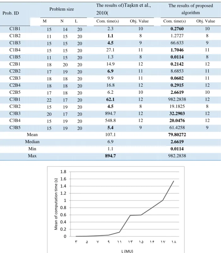
Results of proposed algorithm are given in contrast to study done by Taşkın et al.(2010) for 15 real cases in Table 1. The first column is problem identifier and the second column shows the dimension of problem (𝑀𝑀×𝑁𝑁×𝐿𝐿) in which L stands for maximum value of intensity matrix elements. In addition, computational time and objective function (numbers of segments) are depicted in third and fourth column, respectively.
According to fourth column, both the algorithms provide the same results but average computational time is reduced as much as 25% because of reduction in computational time in nine of the cases. Minimum and median computational times are also reduced in comparison with the best results obtained from literature. But the maximum computational time is not improved using this algorithm. Since the best results of proposed algorithm differ from ones obtained in the literature, it is perceived that for specific kinds of problems, the complexity of both algorithms is increased. In order to investigate the reasons of these exceptional cases and their occurrence reasons, it is needed to be aware of substituted linear solver.
150 random examples generated uniformly in interval [0,𝐿𝐿] and different sizes are solved by proposed algorithm in order to check its behavior in a variety of sizes. Table 2 shows the results of these experiments in four indexes of computational time.
With respect to results shown in Table 2, it seems that the algorithm has a stable behavior in variation of parameter 𝐿𝐿. In such a manner that the mean of computational time for cases with same matrix dimension (𝑀𝑀 =𝑁𝑁 = 5) and two different values of𝐿𝐿 (3 and 18) differs by only 1.5353 seconds. But plotting the computation time vs. parameter 𝐿𝐿(Figure 1) indicates an exponential behavior for algorithm.
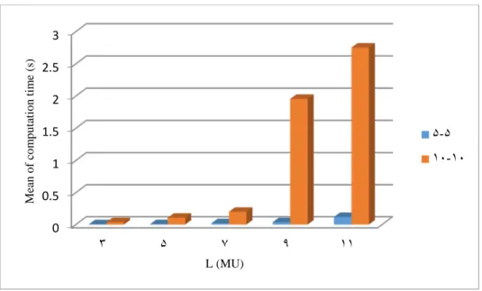
The computation time vs. two different dimensions of intensity matrix in a constant amount of
𝐿𝐿has been plotted in order to analyze its effect as well (Figure 2). Figure 2 not only shows an exponential behavior for differences of computational time but also reveals such a manner for different values of 𝐿𝐿 as well as Figure 1.
Table 1. The results of algorithm in comparison with (Taşkın et al., 2010)
The results of proposed algorithm The results of)Taşkın et al.,
2010( Problem size Prob. ID Obj. Value Com. time(s) Obj. Value Com. time(s) L N M 10 0.2760 10 2.3 20 14 15 C1B1 8 1.2727 8 1.1 20 15 11 C1B2 9 66.633 9 4.5 20 15 15 C1B3 11 1.7046 11 27.1 20 15 15 C1B4 8 0.0114 8 1.3 20 15 11 C1B5 12 0.2142 12 14.9 20 20 18 C2B1 11 8.6853 11 6.9 20 19 17 C2B2 11 0.0602 11 9.9 20 18 18 C2B3 12 0.2915 12 16.8 20 18 18 C2B4 10 2.6619 10 6.2 20 18 17 C2B5 12 982.2838 12 62.1 20 17 22 C3B1 8 19.1825 8 4.5 20 19 15 C3B2 12 32.2903 12 894.7 20 17 20 C3B3 12 20.0476 12 548.8 20 19 15 C3B4 9 61.4258 9 5.4 20 19 15 C3B5 79.80272 107.1 Mean 2.6619 6.9 Median 0.0114 1.1 Min 982.2838 894.7 Max
Figure 1. Behavior of algorithm in terms of maximum element in 𝟓𝟓×𝟓𝟓 random matrixes
0 0.2 0.4 0.6 0.8 1 1.2 1.4 1.6 1.8
۳ ۵ ۷ ۹ ۱۱ ۱۳ ۱۵ ۱۶ ۱۷ ۱۸
M ea n o f c om put at io n tim e ( s) L (MU)
Figure 2. Comparison of computation time between two matrix dimensions 5 × 5 and 10 × 10 vs. different values of parameter 𝐿𝐿
Table2.The results of algorithm for random examples
Computation time Number of Examples Problem dimension Prob. No.
Max Mean Median Min L N M 0.0021 0.0044 0.0039 0.0021 10 3 5 5 1 0.0072 0.0064 0.0061 0.0045 10 5 5 5 2 0.0204 0.0199 0.019 0.0195 10 7 5 5 3 0.0389 0.0369 0.0361 0.0333 10 9 5 5 4 0.182 0.1178 0.0997 0.0362 10 11 5 5 5 0.6177 0.5867 0.3331 0.1799 10 13 5 5 6 0.9308 0.5967 0.383 0.193 10 15 5 5 7 0.8296 0.7971 0.4252 0.0234 10 16 5 5 8 1.0795 1.0048 0.7752 0.6772 10 17 5 5 9 2.6138 1.5397 1.3043 0.1276 10 18 5 5 10 0.0429 0.037 0.013 0.0370 10 3 10 10 11 0.1536 0.1055 0.053 0.1055 10 5 10 10 12 0.2313 0.199 0.0666 0.1990 10 7 10 10 13 2.4992 1.9555 1.1594 1.9555 10 9 10 10 14 3.7481 2.7512 1.2018 2.7512 10 11 10 10 15 0 0.5 1 1.5 2 2.5 3
۳ ۵ ۷ ۹ ۱۱
M ea n of c om put at ion ti m e ( s) L (MU) ۵ -۵ ۱۰ -۱۰
5. Conclusion
In this paper, a new mathematical model is developed for intensity matrix realization in IMRT. This model is linearized through two different techniques and an efficient algorithm is proposed according with them for real size problems. Benders decomposition is applied to obtain the lower bound in this algorithm. Also a new monitor unit sequence generating procedure is introduced.
Results of algorithm for 15 clinical data found in literature (Taşkın et al., 2010) is compared with the best solutions known in terms of objective value and computational time which shows rational superiority of proposed algorithm. Moreover, behavior of algorithm is analyzed along solving 150 other random instances in a spectrum of sizes.
This algorithm can be generalized to handle total treatment time objective function too, by only applying a proper search mechanism. Apart from that some of physical constraints of collimator like interleaf collision constraint, tongue and groove constraint and so on, can be taken into account and added to the model. Furthermore, generating new monitor unit sequences through an evolutionary algorithm seems to be more efficient than doing it in a random manner which can be a direction for future researches.
References
Ahuja, R. K. and Hamacher, H. W., (2005), A network flow algorithm to minimize beam‐on time for unconstrained multileaf collimator problems in cancer radiation therapy,. Networks, 45, 36-41.
Baatar, D., Boland, N., Brand, S. and Stuckey, P. J., (2007), Minimum cardinality matrix decomposition into consecutive-ones matrices: CP and IP approaches, Integration of AI and OR Techniques in Constraint Programming for Combinatorial Optimization Problems. Springer.
Baatar, D., Hamacher, H. W., Ehrgott, M. & Woeginger, G. J.,( 2005), Decomposition of integer matrices and multileaf collimator sequencing., Discrete Applied Mathematics, 152, 6-34.
Bai, L. & Rubin, P. A.,(2009), Combinatorial benders cuts for the minimum tollbooth problem, Operations Research, 57, 1510-1522.
Benders, J. F., (2005), Partitioning procedures for solving mixed-variables programming problems, Computational Management Science, 2, 3-19.
Boland, N., Hamacher, H. W. & Lenzen, F., (2004), Minimizing beam‐on time in cancer radiation treatment using multileaf collimators, Networks, 43, 226-240.
Cambrazard, H., O’mahony, E. & O’Sullivan, B.,(2010), Hybrid methods for the multileaf collimator sequencing problem, Integration of AI and OR Techniques in Constraint Programming for Combinatorial Optimization Problems. Springer.
Cambazard, H., O’mahony, E. & O’Sullivan, B.,( 2012), A shortest path-based approach to the multileaf collimator sequencing problem., Discrete Applied Mathematics, 160, 81-99.
Collins, M. J., Kempe, D., Saia, J. & Young, M.,( 2007), Nonnegative integral subset representations of integer sets, Information Processing Letters, 101, 129-133.
Ehrgott, M., Guller, Ç., Hamacher, H. W. & Shao, L., (2008), Mathematical optimization in intensity modulated radiation therapy. 4OR, 6, 199-262.
Engel, K.,(2005), A new algorithm for optimal multileaf collimator field segmentation, Discrete Applied Mathematics, 152, 35-51.
Ernst, A. T., Mak, V. H. & Mason, L. R., (2009), An exact method for the minimum cardinality problem in the treatment planning of intensity-modulated radiotherapy,. INFORMS Journal on Computing, 21, 562-574.
Gleeson, J. & Ryan, J., (1990), Identifying minimally infeasible subsystems of inequalities,. ORSA Journal on Computing, 2, 61-63.
Kalinowski, T.,(2009), The complexity of minimizing the number of shape matrices subject to minimal beam-on time in multileaf collimator field decomposition with bounded fluence, Discrete Applied Mathematics, 157, 2089-2104.
Mak, V., (2007), Iterative variable aggregation and disaggregation in IP: An application, Operations research letters, 35, 36-44.
Mason, L. R., Mak-Hau, V. H. & Ernst, A. T., (2012), An exact method for minimizing the total treatment time in intensity-modulated radiotherapy, Journal of the Operational Research Society, 63, 1447-1456.
Meyer, J. L., Verhey, L., Pia, L. & Wong, J., (2006), IMRT∙ IGRT∙ SBRT.
Pishvaee, M. S., Razmi, J. & Torabi, S. A., (2014), An accelerated Benders decomposition algorithm for sustainable supply chain network design under uncertainty: A case study of medical needle and syringe supply chain, Transportation Research Part E: Logistics and Transportation Review, 67, 14-38.
Schlegel, W. & Mahr, A., (2007), 3D conformal radiation therapy: Multimedia introduction to methods and techniques, Springer Publishing Company, Incorporated.
Siochi, R. A. C., (1999), Minimizing static intensity modulation delivery time using an intensity solid paradigm, International Journal of Radiation Oncology* Biology* Physics, 43, 671-680.
Taskin, Z. C. & Cevik, M.,(2013), Combinatorial Benders cuts for decomposing IMRT fluence maps using rectangular apertures, Computers & Operations Research, 40, 2178-2186.
Taskin, Z. C., Smith, J. C. & Romeijn, H. E., (2012), Mixed-integer programming techniques for decomposing IMRT fluence maps using rectangular apertures,. Annals of Operations Research, 196, 799-818.
Taskin, Z. C., Smith, J. C., Romeijn, H. E. & Dempsey, J. F.,(2010), Optimal multileaf collimator leaf sequencing in IMRT treatment planning, Operations Research, 58, 674-690.