Sharif University of Technology
Scientia IranicaTransactions E: Industrial Engineering http://scientiairanica.sharif.edu
Research Note
Modeling stock-out loss and overstocking loss generated
by bullwhip eect
M. Zanddizari
a, R. Tavakkoli-Moghaddam
b, and A. Azaron
c;d;1; a. Robert H. Smith School of Business, University of Maryland, College Park, MD, USA.b. Department of Industrial Engineering, College of Engineering, University of Tehran, Tehran, Iran. c. Department of Industrial Engineering, Istanbul Sehir University, Istanbul, Turkey.
d. Beedie School of Business, Simon Fraser University, Vancouver, Canada.
Received 21 July 2017; received in revised form 2 January 2018; accepted 26 February 2018
KEYWORDS Supply chain management; Inventory control; Bullwhip eect; KMV model; Distance to default.
Abstract. Although the literature of the supply chain abounds with the analysis of the bullwhip eect, few studies regarding the impact of the bullwhip eect or demand distortion on the supply chain prot have been done. Hence, the concept of Distance to Loss (DL) is introduced, which is a function of the retailer's selling price, the manufacturer's wholesale price, the end item's salvage value, the retailer's expected demand, and the retailer's variance of demand. This concept can perfectly model both stock-out loss and overstocking loss emanated by the bullwhip eect and combine both the newsvendor model and credit risk concepts. Our ndings are based on an experimental design and are profoundly in line with previous research. In particular, our model indicates that variations in demand parameters, retailer's selling price, and manufacturer's wholesale price impinge on the retailer's DL, whereas a slight increase in the salvage value negligibly aects the retailer's DL.
© 2019 Sharif University of Technology. All rights reserved.
1. Introduction
Presumably, the bullwhip eect, also known as de-mand distortion, has generated many problems for the members of the supply chain since its inception. It negatively aects manufacturing cost, inventory cost, transportation cost, and poor customer service level because of weak product availability and longer lead time [1-3]. On the basis of the bullwhip eect, the protability of the supply chain, due to factors such as price uctuation, order batching, order rationing, and dierent forecasting methods, has signicantly been
1. Present address: School of Business, Kwantlen Polytechnic University, Vancouver, Canada.
*. Corresponding author.
E-mail address: [email protected] (A. Azaron) doi: 10.24200/sci.2018.20199
reduced [4-6]. In other words, as demand distortion is intensied when it passes from one member to another, a tremendous stock-out loss and an overstocking loss are generated for all members of a multi-echelon supply chain [7-11]. Hence, rst, this paper introduces the concept of Distance to Loss (DL) by which we can model both the stock-out loss and the overstocking loss, generated by the bullwhip eect for a retailer. This elegant concept combines the newsvendor model and credit risk concepts. In the second place, this paper investigates how variations in demand parameters as well as prot function variables can aect the stock-out loss and the overstocking loss.
In an eort to ascertain the retailer's prot, we assume that the retailer has a highly uncertain demand, attributed to high overstocking cost and stock-out cost, and is to place his optimal order to a manufacturer for a single selling season as extensively examined in the context of the newsvendor model. Hence, the
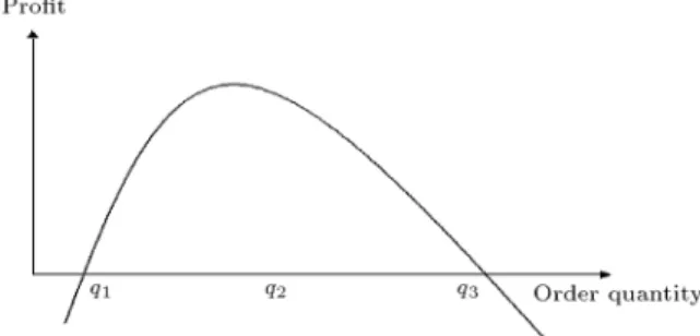
retailer's prot function is attained by striking the balance between the overstocking cost and the stock-out cost and composed of variables like the retailer's order quantity, the retailer's expected demand, the retailer's selling price (p), the manufacturer's wholesale price (c), and the end item's salvage value (s). In addition, the retailer's concave prot function includes three critical points, q1, q2, and q3, see Figure 1.
Under points q1 and q3, the retailer's prot is zero.
We refer to points q1 and q3 as the Breakeven Point
(BP ). In contrast, under point q2, the retailer makes
an optimal prot. On the other hand, the stock-out loss and the overstocking loss occur when expected demand is greater than or less than q2, respectively,
and loss magnitude increases as the expected demand approaches the BP s. As a result, for an expected demand beyond q3or less than q1retailer has a negative
prot or a perfect loss.
The KMV model is a trademark of the KMV Corporation, which was founded by Stephen Kealhofer, John Mcquown, and Oldrich Vasicek in 1989 [12], and is a renowned credit risk model that can estimate nancial loss exposure profoundly [13-22]. For the sake of this paper, we have elicited the DL from the KMV concepts since there is a promising similarity between the DL model parameters and the bullwhip eect parameters. Hence, we have carefully adjusted the DL model to eectively capture the overstocking loss and the stock-out loss, emanated by the bullwhip eect. Our adjusted DL is a function of the expected demand and the variance of demand, p, c, and s. However, since the opportunity cost of a lost customer is somewhat analytically intractable, we have addressed the DL for the stock-out case.
This paper contributes to the literature of the bullwhip eect and the supply chain by rendering the following contributions. First, we have introduced an elegant concept that includes not only the variance of demand as extensively examined in the literature, but also other key related factors, such as selling price, wholesale price, and salvage value. That is, the DL concept highlights other aspects of the bullwhip eect by employing other pertinent factors of demand distortion, such as variations in selling price, wholesale price, and salvage value, in addition to the mean and
Figure 1. The retailer's prot curve.
the variance of demand. Second, our rendered model is capable of capturing both stock-out loss and overstock-ing loss generated by the bullwhip eect. Third, our rendered model is very likely to be generalized to the dierent echelons or supply chains since many supply chains include our model parameters. At last, our model can easily be used by practitioners to magnify the eects of demand distortion on both stock-out loss and overstocking loss.
To arrive at our conclusion, an experimental design is applied to the DL model for a stock-out case. Our ndings are mostly in line with previous ndings in the bullwhip literature. Our results, rstly, indicate that any increase in the expected demand and the variance of demand makes the DL attenuate, which implies a higher likelihood of stock-out loss. Secondly, any decrease in p can result in a lower DL and, im-plicitly, a higher stock-out loss. That is, under a price-dependent demand, low prices induce the demand, and subsequently, lead to a higher likelihood of stock-out. By the same token, an increase in wholesale price is followed by a higher DL and a higher likelihood of stock-out loss. Intuitively, a higher wholesale price implies less retailer prot margin and a lower level of product availability. Nevertheless, one unit increase in variable s does not aect the DL and the stock-out loss, yet increases the retailer's prot. It indicates that a slight increase in s can both enhance the coordination in the supply chain without having an eect on the stock-out loss and improve the retailer's prot.
This paper is organized as follows. Section 2 concisely reviews the bullwhip eect and succinctly delineates KMV concepts. Section 3 models the re-tailer's DL. Sections 4 and 5 include the experimental design and results, respectively. Section 6 presents the conclusion and future research.
2. Literature review 2.1. Bullwhip eect
One of the main consequences of bullwhip eect is excess inventory ow. In fact, when customer's demand passes from one downstream member to an upstream member due to poor communication, the original customer's demand is highly inated when it reaches the last upstream member. This problem is emanated whenever each supply chain member forecasts based on incoming orders. As a result of order ination or mismatch between demand and supply, some members end up with overstocking loss, whereas others incur stock-out loss and experience poor customer service. Furthermore, other detrimental consequences of bull-whip eect such as excess or inadequate capacity along with cost and time of capacity setup, unstable produc-tion planning, and higher transportaproduc-tion, ordering, and holding cost can be seen, too [8,23].
With respect to bullwhip eect, dierent ap-proaches have been utilized to manifest the structure of bullwhip eect and how it negatively aects the supply chain. Simulation-driven studies were origi-nated by Forrester [24,25] and followed by Towill [26] and Wickner et al. [27]. They basically investigated how structure, policies, and communication within a supply chain result in bullwhip eect. In particular, Kim et al. [28] used a simulation model \SISCO" to investigate how stochastic lead times, information sharing, and quality of information aect the supply chain under a periodic order-up-to inventory policy. The second approach, \Beer Game" pioneered by Ster-man [29] and followed by Croson and Donohue [30,31], Haines et al. [32], and Sarkar and Kumar [33] has been mainly used to address the behavioral aspect of bullwhip eect. The third approach initiated by Lee et al. [4,5] introduced four main causes of bullwhip eect such as demand forecast updating (also, [34-37] provide more elaborate analysis about forecasting methods), order ination or order rationing, order batching, and price uctuation, and concluded that these factors methodically impaired the performance of supply chains. In addition, Paik and Bagchi [38] identied other four causes of bullwhip eect such as material delays, information delays, purchasing delays, and levels of echelons; however, only the last one is followed by a very signicant statistical result. Lee and other authors also pinpoint some remedies like uniform and integrated information sharing, order aggregation, and consistent discount programs like Every Day Low Price (EDLP) programs as currently prevalent in many industries in an eort to mitigate the problem. The fourth approach is control system engineering. This approach was addressed by Dejonckheere et al. [8], Sourirajan et al. [39], Salcedo et al. [40], Fu et al. [41], and Wang and Disney [42]. Nonetheless, Miragliotta [43] provided a more elaborate literature review regarding bullwhip eect.
An extensive eort has been exerted by a few researchers such as Metters [44] and Chen et al. [7,45], Kim et al. [28], Frangoo and Wooters [10], Chen and Lee [46], Isaksson and Seifert [47], George and Pil-lai [48], Sodhi et al. [49], and Ma and Bao [50] to quan-tify the bullwhip eect. Metters [44] highlighted how demand seasonality and forecast error could negatively aect the supply chain protability under dierent levels of demand distortion. He used a dynamic pro-gramming model as previously addressed by Zipkin [51] similar to our model, which uses an experimental design to conclude that the bullwhip eect has a negative eect on the supply chain's protability. However, he does not make a distinction between overstocking loss and stock-out loss generated by the bullwhip eect. Hence, our paper has developed the Metters's work by introducing a new elegant concept, DL, into his work
to arrive at a better distinction between overstocking loss and stock-out loss made by the bullwhip eect. In fact, none of the aforementioned studies has made a clear distinction between overstocking loss and stock-out loss, or even rendered an approach to capture them. This research combines the classic newsvendor model with credit risk concept, based on KMV model, to model stock-out loss and overstocking loss in the presence of bullwhip eect. There are many papers on KMV methodology or quantifying bullwhip eect, which were reviewed. However, to the best of our knowledge, these two probabilistic models are com-bined to study the behavior of retailers in a supply chain for the rst time.
2.2. KMV model
On the basis of the KMV methodology, amount of loss exposure in credit risk through some key concepts, such as Distance to Default (DD), Expected Default Frequency (EDF), and Actual Distance to Default (ADD), can be obtained. However, for the sake of this paper, we mainly focus on the DD. That is, we have concisely delineated the concept of DD. In addition, due to profound similarity between KMV model and bullwhip eect structure (stock market volatility and demand distortion), we have elicited the DL from the DD. Below depicts how KMV model and DD are elicited.
As shown in Figure 2, the KMV model includes six variables determining the default probability of a rm over a time horizon up to H as follows [52]:
1. The extant asset value;
2. The distribution of the asset value at time H;
3. The volatility or variance of the future asset value at time H;
4. The level of the default point, which is the book value of the liabilities;
5. The anticipated rate of growth in the asset value over the time horizon;
6. The length of the time horizon, H.
However, by some intermediate calculations, the KMV model follows the probabilities of default, or so-called the Distance to Default (DD) (the distance between the expected asset value in one year and the default point). The DD is the number of standard deviations between the mean and default point. It can be calculated as shown in Eq. (1) [52]:
DD = MV A DP T
MV A V A ; (1)
where:
DP T Default Point (or critical threshold); MV A Market Value of Asset (or current asset
value);
V A Volatility of Asset (or variance of asset).
3. Modeling retailer's DL
In an eort to introduce the DL concept, a combination of the prot function and the KMV approach is applied. To measure the eect of demand distortion on retailer's loss, this paper has recourse to the prot function as a proxy to capture the retailer's loss. To arrive at a perfect prot function, we assume that the retailer incurs high demand uncertainty attributed to both the high overstocking cost and the stock-out cost when retailer selects an optimal order quantity for a single selling season. Hence, the retailer selects an optimal order quantity by striking a balance between the stock-out cost and overstocking cost as seen in the newsvendor model. In fact, our newsvendor model is very similar to the dynamic programming model used by Metters [44] and Zipkin [51]. Furthermore, the stock-out occurs when the expected demand exceeds an optimal order quantity, whereas the overstocking occurs when the expected demand is less than an optimal order quantity.
The net retailer's prot is determined by sub-tracting both the overstocking cost and the stock-out cost from the total prot. Hence, by virtue of a calculated trade-o between the stock-out cost and the overstocking cost, prot equation (Eq. (2)) (the proof is included in Appendix A) as a function of order quantity, stock-out cost, overstocking cost, and demand parameters is determined.
x 2 [a; b]; a; b > 0; and a 6= b; E(x) =a + b2 ; V ar(x) = (b a)12 2; and
f(x) = 1 b a;
0 < s < c < p and p > 2c s;
(x q)+= maxfx q; 0g; and
(q x)+= maxfq x; 0g;
(x q) = (x q)+ (q x)+;
q = total prot-stock-out cost-overstocking cost;
q=(p c)E(x) (p c)E(x q)+ (c s)E(q x)+;
q = cuE(x) cuE(x q)+ coE(q x)+;
q=cu
a+b
2
1
2(b a) cu(q b)2+co(q a)2
: (2) In fact, we assume that the demand is stochastic and follows a uniform distribution. Further, model notations employed in the rest of the paper are dened as follows:
Notations
p Per unit retailer's selling price c Per unit manufacturer's wholesale
price
x Demand
f(x) Uniformly distributed function of demand
a Minimum demand b Maximum demand q Retailer's order quantity E(x) Expected demand V ar(x) Variance of demand
s Per unit item's salvage value cu Stock-out cost
co Overstocking cost
q2 Optimal order quantity
q1 Breakeven point related to overstocking
q3 Breakeven point related to stock-out
The retailer's prot function, Eq. (2), has a concave curve as shown in Figure 1. According to this curve, the retailer has optimal prot at the point q2,
and zero prot at points q1 and q3. Hence, we refer to
points q1and q3as Breakeven Points (BP ), also known
as the default points under KMV model.
When an expected demand is greater than q2, the
retailer faces a stock-out, whereas, when an expected demand is less than q2, the retailer faces an
overstock-ing. However, as the expected demand approaches points q1 and q3, the likelihood of the overstocking
loss and the stock-out loss increases, respectively. In essence, when the expected demand moves either beyond point q3 or below point q1, the retailer makes
a perfect loss. That is, the demand distortion, also known as bullwhip eect, makes the expected demand (or order quantity when it passes to an upstream member) approach either q1 or q3. To arrive at a
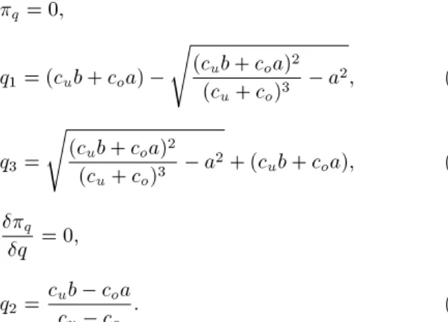
perfect loss estimation, the retailer should judiciously calculate points q1, q2, and q3 based on Eqs. (3)-(5) as
follows (proofs are included in Appendix A). q = 0;
q1= (cub + coa)
s
(cub + coa)2
(cu+ co)3 a
2; (3)
q3=
s
(cub + coa)2
(cu+ co)3 a
2+ (cub + coa); (4)
q
q = 0; q2= cucb coa
u co : (5)
In addition, Eq. (6) includes the optimal prot function under q2 quantity.
q2=cu
a+b
2
1
2(b a) cu(q2 b)2+co(q2 a)2
: (6) Once the above three quantity points are elicited from the retailer's prot function, the derivation of DL becomes possible. That is, as shown in Figure 3, as the demand distortion highly varies, the likelihood of migrating to the loss zones increases. Demand distortion is measured by the variance of demand when it passes from one member to another; in addition, under the uniform distribution, the demand range (b a) is a good indicator of the demand distortion.
Conceivably, the retailer places an optimal order quantity, q2, to the manufacturer well in advance of
selling season. The manufacturer produces q2 and
ships it to the retailer before the actual demand is realized. However, once the actual demand is realized, the retailer compares an actual demand with a pre-dened BP and arrives at the pertinent DL evaluation. In other words, by accruing the sale quantity on the
Figure 3. The retailer's BP s and q2 versus demand
parameters.
monthly basis in a single selling season and comparing it with pre-dened BP , the retailer can attain a perfect and adequate insight into his prot performance. If the DL is attenuating toward the end of selling season, in the case of exposure to the overstocking loss, it is the best strategy for the retailer to either make more eort in the forms of promotions or decrease the price tabs to get the left-over sold. In contrast, in the response to exposure to the stock-out loss, the retailer, at best, can slightly mark up the price tabs to retain his prot margin throughout the selling season.
According to the KMV model, the DL is the distance between the expected demand (E(x)) and BP s. When we take account of q1 (Eq. (3)) as BP ,
DL can capture the overstocking loss, also denoted by DLo, as mentioned in Eq. (7):
DL = E(x) V ar(x)E(x) BP ; DLo=E(x) V ar(x)E(x) q1
=
a+b 2
(cub + coa)
q
(cub+coa)2
(cu+co)3 a2
a+b 2 (b a)
2
12
: (7) In other words, in the case of overstocking, DL is always positive. By contrast, when we assign q3
(Eq. (4)) as BP , DL captures the stock-out loss, also denoted by DLu, as mentioned in Eq. (8):
DLu=E(x) V ar(x)E(x) q3
=
a+b 2
q
(cub+coa)2
(cu+co)3 a2+ (cub + coa)
a+b 2 (b a)
2
12
: (8) Expectedly, under the stock-out loss, DLu is always
negative. By the same token, it is very likely for the retailer to observe both DLoand DLuthroughout the
selling season if he incurs an uncertain demand. On the basis of Eqs. (7) and (8), both DLo and
DLu are a function of the following variables: the
expected demand (a or the minimum demand and b or the maximum demand), the variance of demand, the stock-out cost (cu includes selling price and wholesale
price), and the overstocking cost (coincludes wholesale
price and salvage value). That is, DL models include both the key variables of prot function and the demand distortion variables so as to profoundly model the eect of demand distortion on the retailer's loss.
The expected demand is an average of the ex-pected minimum and the maximum demand and di-rectly aects the retailer's prot. Likewise, the range
of expected demand as the dierence between the maximum and minimum demands is a perfect indicator of the variance of demand under uniform distribution. Hence, the larger expected demand range the retailer has, the smaller is his DL. Nonetheless, this paper is chiey focused on DLu model or Eq. (8) because
of two plausible reasons. First, the opportunity cost of lost customers is somewhat analytically intractable; in addition, the best of our knowledge, few studies regarding the eect of demand distortion on the stock-out loss have been done. Second, all the steps taken to arrive at DLu model are the same as the those to
achieve DLo model or Eq. (7). Hence, in the next
section, an experimental design is presented to evaluate DLu model.
4. Experimental design
In order to highlight the eect of demand distortion on DLu, the retailer's optimal prot, and the retailer's
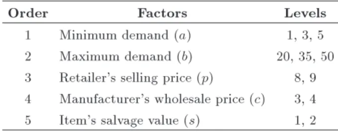
BP , an experiment composed of ve factors is designed. The factors and corresponding levels are presented in Table 1. These factors are key variables in DLu
function and prot function as reviewed in the last section. Likewise, three levels for the minimum and the maximum of demand are chosen to not only reect more explicit demand distortion but also render a more variegated set of expected demand.
In fact, under uniform distribution, the mean and variance of the demand are dened by Factors 1 and 2 as mentioned in Table 1. In addition, dierent combi-nations of Factors 1 and 2 are accompanied by dierent mean and variance of demand as presented in Table 2. The ratio between the lowest and the highest demands is 50:1 with variance 200 which reects the high level of demand distortion, versus 5:20 with variance 18.75, where the retailer faces the lowest demand distortion.
We have also varied the retailer's selling price (p) and manufacturer's wholesale price (c) so as to examine how the promotions and the quantity discount aect
Table 1. The experimental factors and levels.
Order Factors Levels
1 Minimum demand (a) 1, 3, 5 2 Maximum demand (b) 20, 35, 50 3 Retailer's selling price (p) 8, 9 4 Manufacturer's wholesale price (c) 3, 4 5 Item's salvage value (s) 1, 2
the retailer's DLu, the retailer's optimal prot, and
the retailer's BP . Promotion decisions are made by the retailer to induce the demand since any decrease in the prices can generate demand under price-dependent market. In contrast, the manufacturer's wholesale price (c) can aect the quantity and frequency of orders placed by a retailer to a manufacturer. This issue is extensively examined in the context of trade promotion, forward buying, and quantity discount in the supply chain literature.
At last, the value of s is changed slightly to examine how the end item's salvage value (s) aects the retailer's DLu, the retailer's optimal prot, and
the retailer's BP . Conceivably, the higher salvage value is oered by the manufacturer, the greater is the likelihood of order rationing by the retailers as seen in the context of buy-back contracts. In other words, as s increases, the overstocking loss for the retailer reduces conspicuously (the overstocking loss migrates to the manufacturer); in addition, due to higher product availability, the retailer's stock-out loss reduces, too. Hence, it is of high importance to include s among our factors.
For the sake of this paper, 72 experimental cells related to 9 combinations of demand ranges (based on Table 2) times 2 combinations of selling price (based on Table 1) times 2 combinations of wholesale price (based on Table 1) times 2 combinations of salvage value (based on Table 1) are replicated 20 times and examined in the Minitab software to calculate the average of the measures in interest such as retailer's DLu, retailer's optimal prot, and retailer's BP . The
highlights of our results are presented in the next section.
5. Results
Our results report how variations in experimental fac-tors aect the following measures: retailer's DLu,
re-tailer's optimal prot (Eq. (6)), and rere-tailer's BP (q3).
That is, this paper is to investigate how variations in the following factors, i.e., demand parameters, selling price, wholesale price, and salvage value, respectively, discussed in the following sections, can aect the above measures.
5.1. Variations in the range of expected demand
Intuitively, as the range of expected demand decreases,
Table 2. Combinations of demand ranges and related mean and variance. (a,b) (1,20) (1,35) (1,50) (3,20) (3,35) (3, 50) (5,20) (5,35) (5,50)
E(x) 10,5 18 25.5 11.5 19 26.5 12.5 20 27.5
Figure 4. Changes in the retailer's DLudue to variations
in demand parameters.
Figure 5. Changes in the retailer's optimal prot due to variations in demand parameters.
Figure 6. Changes in the retailer's BP (q3) due to
variations in demand parameters.
the variance of demand decreases. Reduction in the variance of demand results in an increase in the retailer's DLuas seen in Figure 4.
Likewise, as the range of demand migrates from a low range to a high range like (1,20) to (1,50), or (3,20) to (3,50) or (5,20) to (5,50), the retailer's DLu dramatically reduces. This reduction in the
retailer's DLu implies a higher likelihood of
stock-out loss. Hence, the retailer's DLu model perfectly
highlights the eect of demand distortion on the stock-out loss. Figures 5 and 6 show how the retailer's optimal prot and the retailer's BP react to the vari-ations of the demand range, respectively. According to Figure 5, surprisingly, the level of retailer's optimal prot decreases in spite of an increase in the retailer's
Figure 7. Changes in the retailer's DLudue to variations
in p, c, and s.
DLu as the demand range is attenuated. There are
two plausible reasons that can explain the behavior of retailer's optimal prot. First, as the expected demand reduces, the retailer's BP reduces accordingly as shown in Figure 6, which has counter-productive eect on the retailer's DLu. Second, conceivably, as the range of
demand decreases, the range of expected sale decreases, accordingly. Hence, under a lower demand range, the retailer makes less prot.
It is of high importance to strike the balance between risk and return. That is, under the high range of demand, the retailer is exposed to high demand uncertainty, but at the expense of apparently higher sale or prot. This trade-o can easily be tracked in Figures 4 and 5. These results indicate that the retailer's DLu is a reliable indicator of demand
distortion since it includes two key factors such as the variance of demand and the expected demand. 5.2. Variations in the retailer's selling price
(p)
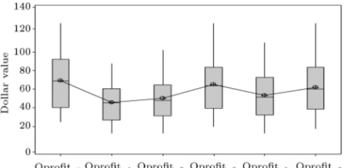
Presumably, one of the main causes of the demand distortion or the bullwhip eect is the price uctuation engendered by the retailer. In essence, the initiation of unilateral promotions by the retailer makes lumpy demand attributed to the forward buying behavior of nal customers. Consequently, this lumpy demand is amplied when it is passed to the upstream members. As shown in Figure 7, an increase in the price, from $8 to $9, can lead to a higher retailer's optimal prot as shown in Figure 8, and lowering retailer's DLu, mainly
due to an increase in the retailer's BP, as shown in Figure 9. Lowering retailer's DLu, mainly due to an
increase in the retailer's BP , Presumably, our results shed light on the inverse relationship between selling price and stock-out loss and direct relationship between selling price and retailer's prot. That is, as long as market has the price-dependent demand, higher prices end up with tremendous loss for the retailer toward the end of selling season. In practice, the retailer can mark up his prices at the outset of selling season and reduce them gradually toward the end of selling season to retain an appropriate level of prot.
Figure 8. Changes in the retailer's optimal prot due to variations in p, c, and s.
Figure 9. Changes in the retailer's BP (q3) due to
variations in p, c, and s.
5.3. Variations in the manufacturer's wholesale price (c)
It stands to reason that a lower wholesale price implies a higher retailer's prot margin. Wholesale price has extensively examined in the context of supply chain contracting for the sake of channel coordination. In particular, under the trade promotion and quantity discount contacts, the manufacturer is willing to oer a lower wholesale price for the retailer in an eort to entice the retailer to sell through. However, the retailer makes forward buying as extensively seen in commodity products. The forward buying or sell-in can intensify the demand distortion. In other words, a decrease in wholesale price from $4 to $3 leads to a lower retailer's DLu (or a lower likelihood of stock-out) as shown in
Figure 7, a higher retailer's optimal prot as shown in Figure 8, and a higher level of retailer's BP , as shown in Figure 9. It means that the large reductions in wholesale price result in sell-in rather than sell-through and, consequently, lead to the demand distortion. 5.4. Variations in the end item's salvage value
(s)
Salvage value is dened as a fraction of wholesale price by the manufacturer. That is, the manufacturer is will-ing to buy back the left-over at the end of sellwill-ing season by paying a fraction of end item's wholesale price to the retailer. The higher fraction means the higher willingness to share the risk by the manufacturer and implicitly the lower stock-out loss and the overstocking
loss for the retailer. That is, an increase in salvage value implies that the manufacturer is willing to take on some risks associated with the demand uncertainty, leading to an increase in the retailer's prot.
Nonetheless, the retailer can take advantage of a higher salvage value by placing inated orders to the manufacturer. This issue has been extensively discussed in the context of quantity exibility contract and buy-back contract where the manufacturer denes a set of competitive s in the hope of coordinating the supply chain. However, a higher salvage value oered to the retailer means less overstocking loss and a higher level of product availability for the retailer. Hence, these conspicuous benets of a higher salvage value induce the retailer to inate his orders above the real expected demand and bring on the demand distortion in the supply chain.
As salvage value increases from $1 to $2, the retailer's optimal prot increases, as shown in Figure 8. However, the levels of the retailer's BP and the retailer's DLu are the same in both salvage values,
as shown in Figures 9 and 7, respectively. In fact, a negligible change in the retailer's DLu and the
retailer's BP stems from a slight increase in salvage value. Hence, it indicates that a slight increase in salvage value is innocuous for the supply chain while it improves the retailer's prot.
6. Conclusion
This study introduced an ecient approach to model both the stock-out loss and the overstocking loss in the presence of bullwhip eect. To have our model prociently reect the retailer's loss due to the bullwhip eect, we have recourse to both the newsvendor model and well-established credit risk concepts. Hence, we arrived at three important models such as the retailer's prot function, the retailer's BP , and the retailer's DL; most variables embedded in our models are in connection with bullwhip eect context.
This paper contributes to the literature of bull-whip eect and the supply chain by rst including not only the mean and variance of demand, but also other key related factors such as selling price, wholesale price, and salvage value in our models. Second, our models are capable of capturing both the stock-out loss and the overstocking loss generated by the bullwhip eect. Third, our models are very likely to be generalized to dierent supply chain settings due to our applicable model parameters. At last, our models can easily be used by the practitioners to pinpoint the eect of demand distortion on both their stock-out loss and the overstocking loss.
Our ndings are reported based on an experimen-tal design and are mostly in line with previous ndings in the bullwhip literature. Our results indicate, rstly,
that any increase in the expected demand and the variance of demand makes the retailer's DL attenuate, which implies a higher likelihood of stock-out loss. Secondly, a decrease in selling price can result in a lower retailer's DLu and implicitly a higher stock-out
loss. Likewise, a decrease in wholesale price is followed by a lower DLu of the retailer and a lower likelihood
of stock-out loss. Intuitively, a higher wholesale price implies a less retailer's prot margin and a lower level of product availability. Nevertheless, one unit increase in salvage value barely aects the retailer's DLu and
the retailer's stock-out loss, but increases the retailer's prot. It indicates that a slight increase in salvage value can both enhance the coordination in the supply chain without having eect on the stock-out loss and improve the retailer's prot.
Since this paper has mainly focused on the intro-duction of DL into the context of bullwhip eect and supply chain, there are some conspicuous potentials for the future research. Firstly, we merely examined the retailer's loss rather than tracking a multi-echelon supply chain loss by comparing the DL of one member with another. Hence, applying the DL concept in a multi-echelon supply chain will be a creditable future research subject. Secondly, another track of research is to examine the impact of bullwhip eect on DLo
and compare the ndings with our paper results. Thirdly, for the sake of simplicity, we used a uniform distribution for the demand that might dier from real demand distributions attributed to high skewness. Therefore, the examination of lognormal distribution or worst-case distribution (for highly volatile demands) instead of uniform distribution can accompany more realistic results.
References
1. Chopra, S. and Meindel, P., Supply Chains Manage-ment, 2nd Ed., Prentice-Hall Co. (2004).
2. Stock, J.R. and Lambert, D.M., Strategic Logistic Management, 4th Ed., McGraw-Hill Co. (2001).
3. Poirier, C.C., Advance Supply Chain Management, 1st Indian Ed., Berret-Koehler Publisher, Inc. (2002).
4. Lee, H., Padmanabhan, V., and Wang, S. \The bullwhip eect in supply chains", Sloan Management Review, 38, pp. 93-102 (1997).
5. Lee, H., Padmanabhan, V., and Wang, S. \Information distortion in a supply chains: the bullwhip eect", Management Science, 43, pp. 546-558 (1997).
6. Cambridge, M.A. and Kahn, J.A. \Inventories and the volatily of production", American Economic Review, 174, pp. 667-679 (1987).
7. Chen, Y.F., Drezner, Z., Ryan, J.K., and Simchi-Levi, D. \Quantifying the bullwhip eect in a simple supply chains: The impact of forecasting, lead-times
and information", Management Science, 46, pp. 436-443 (2000).
8. Dejonckheere, J., Disney, S.M., Lambrecht, M.R., and Towill, D.R. \Measuring and avoiding the bullwhip ef-fect: A control theoretic approach", European Journal of Operational Research, 147, pp. 567-590 (2003).
9. Eichenbaum, M.S. \Some empirical evidence of the production level and production cost smoothing mod-els of inventory investment", American Economic Re-view, 79, pp. 853-864 (1989).
10. Frangoo, J.C. and Wooters, M.J.F. \Measuring the bullwhip eect in the supply chains", Supply Chains Management, 5, pp. 78-89 (2000).
11. Khan, A. and Thomas, J.K. \Inventories and the business cycle: An equilibrium analysis of (S,s) poli-cies", Federal Reserve Bank of Minneapolis, Research Department Sta Report 329 (2003).
12. KMV Corporation, Credit Monitor Overview, San Francisco, CA (1993).
13. Kealhofer, S., Measuring Default Risk in Portfolios of Derivatives, Mimeo KMV Corporation", San Fran-cisco, CA (1996).
14. Crouhy, M., Galai, D., and Mark, R. \A comparative analysis of current credit risk models", Journal of Banking and Finance, 24, pp. 59-117 (2000).
15. Altman, E.I. and Saunders, A. \Credit risk measure-ment: Developments over the last 20 years", Journal of Banking and Finance, 21, pp. 1721-1742 (1997).
16. Scott, J. \The probability of bankruptcy: A compari-son of empirical predictions and theoretical models", Journal of Banking and Finance, 5, pp. 317-344 (1981).
17. Carey, M. and Hrycay, M. \Parameterizing credit risk models with rating data", Journal of Banking and Finance, 25, pp. 197-270 (2001).
18. Li, L., Yang, J., and Zou, X. \A study of credit risk of Chinese listed companies: ZPP versus KMV", Applied Economics, 48, pp. 2697-2710 (2016).
19. Norliza, M.Y. and Maheran, M.J. \Forecasting the probability of default of PN17 company using KMV-Merton model", International Journal of Applied Mathematics & Statistics, 53, pp. 103-108 (2015).
20. Lee, W.C. \Redenition of the KMV model's optimal default point based on genetic algorithms - Evidence from Taiwan", Expert Systems with Applications, 38, pp. 10107-10113 (2011).
21. Zhang, Y. and Shi, B. \Non-tradable shares pricing and optimal default point based on hybrid KMV mod-els: Evidence from China", Knowledge-Based Systems, 110, pp. 202-209 (2016).
22. Ching-Chiang, Y., Fengyi, L., and Chih-Yu, H. \A hybrid KMV model, random forests and rough set theory approach for credit rating", Knowledge-Based Systems, 33, pp. 166-172 (2012).
23. Machuca, J.A.D. and Barajas, R.P. \The impact of electronic data interchange on reducing bullwhip eect and supply chains inventory costs", Transportation Research Part E: Logistics and Transportation Review, 40, pp. 209-228 (2004).
24. Forrester, J.W. \Industrial dynamics - A major break-through for decision makers", Harvard Business Re-view, 36, pp. 37-66 (1958).
25. Forrester, J.W., Industrial Dynamics, MIT Press and John Wiley & Sons, Inc., New York (1961).
26. Towill, D. \Supply chain dynamics", International Journal of Computer Integrated Manufacturing, 4, pp. 197-208 (1991).
27. Wickner, J., Towill, D.R., and Naim, M. \Smoothing supply chain dynamics", International Journal of Pro-duction Economics, 22, pp. 231-248 (1991).
28. Kim, J.G., Chateld, D., Harrison, T.P., and Hayya, J.C. \Quantifying the bullwhip eect in a supply chain with stochastic lead time", European Journal of Operational Research, 173, pp. 617-636 (2006).
29. Sterman, J.D. \Modeling managerial behavior: Mis-perceptions of feedback in a dynamic decision making experiments", Management Science, 35, pp. 321-339 (1989).
30. Croson, R. and Donohue, K. \Behavioral causes of the bullwhip eect and the observed value of inventory information", Management Science, 52, pp. 323-336 (2006).
31. Croson, R. and Donohue, K. \Impact of POS data sharing on supply chain management: An experimen-tal study", Production and Operations Management, 12, pp. 1-11 (2003).
32. Haines, R., Hough, J., and Haines, D. \A metacogni-tive perspecmetacogni-tive on decision making in supply chains: Revisiting the behavioral causes of the bullwhip ef-fect", International Journal of Production Economics, 184, pp. 7-20 (2017).
33. Sarkar, S. and Kumar, S. \A behavioral experiment on inventory management with supply chain disruption", International Journal of Production Economics, 169, pp. 169-178 (2015).
34. Zhang, X. \The impact of forecasting methods on the bullwhip eect", International Journal of Production Economics, 88, pp. 15-27 (2004).
35. Sadeghi, A. \Providing a measure for bullwhip eect in a two-product supply chain with exponential smooth-ing forecasts", International Journal of Production Economics, 169, pp. 44-54 (2015).
36. Khosroshahi, H., Moattar Husseini, S.M., and Marjani, M.R. \The bullwhip eect in a 3-stage supply chain considering multiple retailers using a moving average method for demand forecasting", Applied Mathemati-cal Modelling, 40, pp. 8934-8951 (2016).
37. Sirikasemsuk, K. and Luong, H.T. \Measure of bull-whip eect in supply chains with rst-order bivari-ate vector autoresgression time-series demand model", Computers & Operations Research, 78, pp. 59-79 (2017).
38. Paik, S.K. and Bagchi, P. \Understanding the causes of the bullwhip eect in a supply chain", International Journal of Retail & Distribution Management, 35, pp. 308-324 (2007).
39. Sourirajan, K., Ramachandran, B., and An, L. \Appli-cation of control theoretic principles to manage inven-tory replenishment in a supply chain", International Journal of Production Research, 46, pp. 6163-6188 (2008).
40. Salcedo, C.A.G., Hernandez, A.I., Vilanova, R., and Cuartas, J.H. \Inventory control of supply chains: Mit-igating the bullwhip eect by centralized and decen-tralized internal model control approaches", European Journal of Operational Research, 224, pp. 261-272 (2013).
41. Fu, D.F., Ionescu, C., Aghezzaf, E.H., and Keyser, R.D. \Quantifying and mitigating the bullwhip eect in a benchmark supply chain system by an extended prediction self-adaptive control ordering policy", Com-puters & Industrial Engineering, 81, pp. 46-57 (2015).
42. Wang, X. and Disney, S.M. \Mitigating variance amplication under stochastic lead-time: The propor-tional control approach", European Journal of Opera-tional Research, 256, pp. 151-162 (2017).
43. Miragliotta, G. \Layers and mechanisms: A new tax-onomy for the bullwhip eect", International Journal of Production Economics, 104, pp. 365-381 (2006).
44. Metters, R. \Quantifying the bullwhip eect in supply chain", Journal of Operation Management, 15, pp. 89-100 (1997).
45. Chen, F., Ryan, J.K., and Simchi-Levi, D. \The impact of exponential smoothing forecasts on the Bullwhip Eect", Naval Research Logistics, 47, pp. 269-286 (2000).
46. Chen, L. and Lee, H.L. \Information sharing and order variability control under a generalized demand model", Management Science, 55, pp. 781-797 (2009).
47. Isaksson, O.H.D. and Seifert, R.W. \Quantifying the bullwhip eect using two-echelon data: A cross-industry empirical investigation", International Jour-nal of Production Economics, 171, pp. 311-320 (2016).
48. George, J. and Pillai, V.M. \Transfer function models of inventory policies and bullwhip quantication in supply chain", Procedia Technology, 25, pp. 1064-1071 (2016).
49. Sodhi, M.S., Sodhi, N.S., and Tang, C.S. \An EOQ model for MRO customers under stochastic price to quantify bullwhip eect for the manufacturer", Inter-national Journal of Production Economics, 155, pp. 132-142 (2014).
50. Ma, J. and Bao, B. \Research on bullwhip eect in energy-ecient air conditioning supply chain", Journal of Cleaner Production, 143, pp. 854-865 (2017).
51. Zipkin, P.H. \Critical number policies for inventory models with periodic data", Management Science, 35, pp. 71-80 (1989).
52. Moody's KMV Company, Modeling Default Risk, Mod-eling Methodology (2003).
Appendix A
Below are the proofs of Eqs. (2)-(5):
q = cuE(x) cuE(x q)+ coE(q x)+;
q = cuE(x) cu b Z q (x q)f(x)dx co q Z a (x q)f(x)dx;
q = cu
a + b
2 cu b Z q (x q) b a dx co
q
Z
a
(q x) b a dx; q = cu
a + b
2
1 2(b a)
cu(q b)2
+co(q a)2
; q = 0;
cu
a + b
2
= 1
2(b a) cu(q b)2+ co(q a)2
; (cu(q b)2+ co(q a)2) = cu(b2 a2);
q1;3=
r
cu(b2 a2) (cub2+coa2)+
cub+coa
cu+co
2
+cpub+coa
cu+co
p
cu+co ;
q1= (cub + coa)
s
(cub + coa)2
(cu+ co)3 a 2;
q3=
s
(cub + coa)2
(cu+ co)3 a
2+ (cub + coa);
q
q = 0; q2=cucb coa
u co ;
q2 = cu
a + b
2
1
2(b a)(cu(q2 b)2 +co(q2 a)2):
Biographies
Mahdi Zanddizari is a PhD candidate in Robert H. Smith School of Business at University of Maryland in the US. He obtained his MSc degree in Industrial Engineering at Mazandaran University of Science and Technology in Iran in 2006. His research works appeared in a number of conference proceedings with peer reviews including MS'06 Proceedings of the 17th IASTED International Conference on Modelling and Simulation.
Reza Tavakkoli-Moghaddam is a Professor of In-dustrial Engineering at College of Engineering, Uni-versity of Tehran in Iran. He obtained his PhD in Industrial Engineering from Swinburne University of Technology in Melbourne (1998), his MSc in Industrial Engineering from the University of Melbourne in Mel-bourne (1994), and his BSc in Industrial Engineering from the Iran University of Science and Technology in Tehran (1989). He serves as a member of the Editorial Board of ve reputable academic journals. He is the re-cipient of the 2009 and 2011 Distinguished Researcher Awards and the 2010 and 2014 Distinguished Applied Research Award at University of Tehran, Iran. He has been selected as the National Iranian Distinguished Researcher for 2008 and 2010. He has published 4 books, 15 book chapters, and more than 600 journal and conference papers.
Amir Azaron currently holds a Visiting Associate Professor position in the Beedie School of Business at Simon Fraser University in Vancouver, Canada. He holds two PhD degrees: the rst in Industrial Engi-neering obtained from Tarbiat Modarres University in Iran in 2000 and the second in Systems Engineering obtained from Hiroshima University in Japan in 2005.
His research interests include multiple objective deci-sion making, stochastic networks, supply chain man-agement, reliability, production planning, and project management. He held various positions in more than 10 academic institutions in North America, Europe, and Asia. His research works appeared in a number of
top operations research/management science journals including European Journal of Operational Research, Or Spectrum, Annals of Operations Research, Com-puters & Operations Research, ComCom-puters & Indus-trial Engineering, International Journal of Production Economics, etc.