Sharif University of Technology
Scientia IranicaTransactions A: Civil Engineering http://scientiairanica.sharif.edu
Numerical modeling of ood waves in a bumpy channel
with dierent boundary conditions
S. Farmani
, Gh. Barani, M. Ghaeini-Hessaroeyeh, and R. Memarzadeh
Department of Civil Engineering, Faculty of Engineering, Shahid Bahonar University of Kerman, Kerman, P.O. Box 76169-133, Iran.
Received 26 November 2016; received in revised form 1 July 2017; accepted 3 November 2017
KEYWORDS Flood waves; ISPH method; Wave breaking; Uneven bed; Fractional method.
Abstract. In this paper, the Incompressible Smoothed Particle Hydrodynamics (ISPH) method is presented to simulate ood waves in uneven beds. The SPH method is a mesh-free particle modeling approach that is capable of tracking large deformation of mesh-free surfaces in an easy and accurate manner. Wave breaking is one of the phenomena whose free surface is complicated. Therefore, ISPH method is a robust tool for the modeling of this kind of free surface. The basic equations are the incompressible mass conservation and Navier-Stokes equations that are solved using a two-step fractional method. In the rst step, these equations are solved to compute velocity components by omitting the pressure term in the absence of an incompressible condition. In the second step, the continuity constraint is satised and the Poisson equation is solved to calculate pressure terms. In the present model, a new technique is applied to allocate density of the particles for the calculations. By employing this technique, ISPH method is stable. The validation by comparison with laboratory data is conducted for bumpy channel with various boundary conditions. The numerical results showed good agreement with available experimental data. In addition, relative error is calculated for two numerical cases.
© 2019 Sharif University of Technology. All rights reserved.
1. Introduction
Flood wave is a complex phenomenon that occurs in free surface ows with large deformation. Dam break wave is one of such ows that can cause losses and damages. Therefore, the prediction of the water level position, velocity, and pressure is essential. These problems are dicult to simulate due to the existence of the arbitrarily moving surface boundary conditions and also because of the complex governing Navier Stokes Equations (NSEs) [1]. Therefore, the dam
*. Corresponding author. Tel.: +98-34-32650724 E-mail addresses: [email protected] (S. Farmani); [email protected] (Gh. Barani); [email protected] (M. Ghaeini-Hessaroeyeh);
[email protected] (R. Memarzadeh) doi: 10.24200/sci.2017.4582
break problem has been the subject of many analytical, experimental, and numerical studies for hydraulics scientists and engineers [2-4]. The marker and cell [5] and Volume Of Fluid (VOF) [6] methods are the most common methods for simulating such ows, in which the Navier-Stokes equations are solved on a xed Eulerian grid [7]. In MAC method, marker particles are used to dene the free surface, while, in VOF method, the governing equations are solved for the volume fraction of the uid. However, in spite of successful use of both methods for treating free surface ows, numerical diusion arose due to solving NSEs on a xed Eulerian grid, especially when the deformation of free surface is very large [8]. In the general area of computational mechanics, there is a growing interest in developing so-called meshless/mesh-free methods or particle methods as alternatives to traditional grid-based methods such as nite dierence methods and
nite-element methods [9]. One of the oldest mesh-less methods is the Smoothed Particle Hydrodynamics (SPH) method. Smoothed particle method is originally used for astronomic problems. Recently, this method has been well studied and applied in computational uid dynamics, especially for ows with complex free surface [10]. Furthermore, SPH method was used successfully to model the xed-bed dam break ow on dry-bed and wet-bed downstream channels [11,12]. Ozbulut et al. [13] carried out a numerical investigation into the correction algorithms for SPH method in modelling violent free surface ows.
SPH simulations of the incompressible ows can be carried out by two approaches:
1. Approximately simulating incompressible ows with small compressibility, or Weakly Compressible SPH (WCSPH);
2. Simulating ows by enforcing incompressibility, or Incompressible SPH (ISPH).
In WCSPH method, the ow is considered as slightly compressible, with a state equation for the pressure calculation [14,15]. In ISPH method, the pressure-velocity coupling is generally solved by the projection method [16-19].
In this eld, Xenakis et al. [20] improved the pres-sure predictions using an incompressible SPH scheme for free surface Newtonian ows. Nomeritae et al. [21] presented an explicit incompressible SPH algorithm for free surface ow and, then, compared this algorithm with weakly compressible scheme.
This paper presents an incompressible 2D ISPH model to simulate ood waves in uneven bed and validated in Sections 5 for a rough bumpy channel with various boundary conditions. Furthermore, the relative error is calculated in a dierent section.
2. Governing equations
The Navier-Stokes equations (mass and momentum conservation equations) are written in 2D Lagrangian form as follows [3]:
1
D
Dt + r:u = 0; (1)
Du Dt =
1 rp +
r2u + fb; (2) where is the ow density, u is the ow velocity, p is the pressure, is dynamic viscosity, fb represents
the body force, and t is time. Eq. (1) is in the form of a compressible ow. Incompressibility is enforced in a correction step of the time integration by setting
D
Dt = 0 at each particle. The motion of each particle
is calculated by Dr=Dt = u, with r being the position vector. These equations are solved by SPH method.
3. Numerical methodology 3.1. ISPH formulations
In the SPH method, nodal points that are scattered in space with no denable grid structure and move with the uid represent the uid domain. Each of these nodal points has information, such as density, pressure, velocity components, etc. [22]. The SPH formulation is obtained as a result of interpolation between a set of disordered points known as particles. The interpolation is based on the theory of integral interpolants that uses a kernel function to approximate delta function. The kernel approximation of f is written in the form [23]:
f(r) = Z
f(r)W (jr r_ 0j ; h) dr: (3)
In the particle approximation, for any function of eld variable:
f(ri) = n
X
j=1
mj
jf(rj) _
W (jri rjj ; h) ; (4)
where is the support domain, mjand jare the mass
and density of particle j, mj=j is the volume element
associated with particle j,W is the interpolation kernel_ function (in this paper, kernel based on the spline function is used [23]), r is the position vector, h is the smoothing distance which determines width of kernel and, ultimately, the resolution of the method and in this paper h = 1:2 dr where dr is the initial particle spacing, and n is the total number of particles within the smoothing that aects particle i. For example, density of a particle in the SPH approximation is represented as follows:
i = n X j=1 mj _
W (jri rjj ; h) : (5)
The formulation of the gradient term has dierent forms depending on the derivation used [23]. The gradient of the pressure is expressed as follows:
1
i(rPi) =
X
j
mj P2j j +
Pi
2 i
!
rWij; (6)
where P is pressure of the particles.
Similarly, the divergence of vector u at particle i can be expressed by:
r:~ui= i
X
j
mj ~u2i i +
~uj
2 j
!
:riWij: (7)
The Laplacian for the pressure and viscosity term is formulated as the hybrid of a standard SPH rst derivative coupled with a nite dierence approxima-tion for the rst derivative [4]. Furthermore, it has been found that the resulting second derivative of the kernel is very sensitive to particle disorder and will
easily lead to pressure instability and decoupling in the computation due to the co-location of the velocity and pressure [8]. These are represented by:
r: 1 rP i =X j
mj( 8 i+ j)2
Pijrij:riWij
jrijj2+ 2 ; (8)
r2u
i=
X
j
4mj(i+j)rij:ri _
Wij
(i+j)2(jrijj2+2) (ui uj); (9)
where Pij = Pi Pj, rij = ri rj, is the viscosity
coecient, and is a small number introduced to keep the denominator non-zero during computation and is usually equal to 0:1h. After employing the SPH formulation in Eq. (9) for the Laplacian of pressure, the corresponding coecient matrix of linear equations is symmetric and positive denite and can be eciently solved by available solvers.
3.2. Limitation of time step
In the simulation of water ows, in which the uid vis-cosity is not a control factor, the stability of the ISPH computation requires the following Courant condition to be observed:
t 0:1vx
max; (10)
where vmax denotes the maximum particle velocity in
the computational domain. Factor 0.1 ensures that the particle moves only a small fraction of the particle spacing per time step [24].
3.3. Boundary conditions 3.3.1. Free surface boundary
The ISPH model uses the particle density to judge the free surface, and a zero pressure is given to these particles. The criterion is that there is no uid particle existing in the outer region of the free surface; therefore, the particle density on the surface should drop signicantly [8]. Therefore, a particle which satises the following equation was considered to be on the free surface:
()i< (0)i: (11)
In this equation, is the free surface parameter and 0:8 < < 0:99 [25]. In this paper, = 0:94 is used. Eq. (11) is applied to the free surface particles in order to move correctly, avoid instability in the computations, and control their incompressibility condition [1].
3.3.2. Solid wall boundaries
Solid walls are simulated by one line of particles. In order to satisfy the non-slip boundary condition, the velocities of wall particles are set to zero. To balance the pressure of inner uid particles and prevent them from penetrating the solid walls, the pressure Poisson
equation is solved for these wall particles, and the Neumann boundary condition is imposed. In addition, two lines of dummy particles are placed outside wall boundaries and their pressure is set to that of a wall particle in the normal direction of the solid walls. By imposing these conditions, the density of particles is computed accurately, and wall particles are not considered as free surface particles [8].
4. Solution algorithm
At rst, the initial conditions, such as problem geom-etry, smoothing distance, number of particles, mass, dynamic viscosity, initial, coordinate, and their velocity are dened. Then, two-step fractional algorithm is applied. In the rst step, the Navier Stokes equations are solved to compute velocity components without the pressure term in the absence of incompressible condition. In the second step, the continuity constraint is satised, and the resulting Poisson equation is solved to calculate pressure terms [8]. This algorithm can be summarized in ve stages:
- The density of the particles using the following equation is calculated [8]:
0 i = X j mj _
W (jri rjj ; h) : (12) - The prediction step: Temporary particle positions and velocities by considering the gravity and viscos-ity terms in Eq. (2) are computed [8]:
~u=
~g +
r2u
t; (13)
u= ut+ u; (14)
r= r
t+ ut; (15)
where utand rtare the particle velocity and position
at time t; u and r are the temporary particle
ve-locity and position, respectively, and uis changed
in the particle velocity during the prediction step. In this step, due to omitting the pressure term, the uid density is changed and computed again by Eq. (16). Therefore, incompressibility is not still satised [8].
i = X j mj _ W r
i rj;h: (16)
- The correction step: in this step, the pressure term is computed through Poisson equation (Eq. (19)) by considering the continuity constraint and enforcing incompressibility with combining Eqs. (17) and (18) as follows [8]:
1 0
0
u= 1
rPt+1t; (18)
r:
1 rPt+1
=0
0t2 : (19)
The Poisson equation produces a system of linear equation solved by iterative solvers.
- New particle velocities are obtained from Eqs. (19) and (20) [8]:
ut+1= ut+ u: (20) - The new position of particles is computed by
Eq. (21) [8].
rt+1= rt+ut+12+ utt: (21)
5. Numerical validations
In this section, the numerical accuracy and applica-bility of the proposed ISPH method are examined by the laboratory measurements of dam-break ows in the bumpy channel.
5.1. Dry bed with open end
5.1.1. Problem geometry and solution domain
In this case, the experimental data of Ozmen-Cagatay et al. [26] are used. Dimensions of the channel and reservoir are displayed in Figure 1. The bed is totally dry before and after the obstacle, and there is an open end boundary condition.
5.1.2. Qualitative description of the ow
After lifting the gate, the water wave propagates over the bed. After about t = 0:9 s, the ow water hits the obstacle. At t = 1:36 s, amount of water passes the bump, while, at t = 2:8 s, the wave reection of the bump is clearly observed. The water ow and propagation of waves are shown in Figure 2 for t = 0:22 s, t = 0:5 s, t = 0:9 s, t = 1:36 s, t = 2:8 s, t = 3:3 s, t = 3:68 s, t = 4:74 s, and t = 5:72 s. The good agreement exists between the present model results and the experimental data.
5.1.3. Comparison of free surface prole with experimental data
The free surface proles are shown in Figure 3, and the results of the present model are compared with exper-imental data of Ozmen-Cagatay et al. [26]. Of note,
Figure 1. The initial geometry of the bumpy channel with dry bed [26].
Figure 2. The free surface proles and pressure eld in the present model and the experimental data of
Ozmen-Cagatay et al. [26] at dierent times for bumpy channel with dry bed.
Figure 3. Comparison of the free surface prole between the present model results and the experimental data of Ozmen-Cagatay et al. [26] at dierent dimensionless times: (a) T = 15:16, (b) T = 17:54, (c) T = 20:67, (d)
T = 23:05, (e) T = 29:69, (f) T = 35:83, (g) T = 41:84, and (h) T = 49:99.
the space and the level of water are dimensionless and the time is multiplied by (g=ho)0:5; then, dimensionless
time, T = t(g=ho)0:5, is obtained (g and ho are gravity
acceleration and initial depth of water, respectively). According to Figure 3, at T = 15:16 and T = 17:54 as well as on the top of the obstacle, the estimate of water level of the numerical model is slightly higher than that of the experimental data of Ozmen-Cagatay et al. [26]. However, in both cases, the maximum of the water depth occurred on the peak of the bump (bump is a triangular obstacle shown in Figure 3). At T = 20:67, from the rst of the bed up to the end of the bump, the numerical model slightly overestimates the water level. From T = 20:67 up to T = 35:83, when the ow wave reaches the bump, part of water is reected and another part passes the bump. At T = 23:05 before the obstacle, the free surface prole of the present model is higher than that of the experimental data. At T = 29:69 and T = 35:83, the water level at the upstream of the bump is changeless in the numerical model. At the time progress (T > 35:83), the water level is maximum at the top of the bump. At T = 41:84 and T = 49:99, the results of the present model are in good agreement with the experimental data.
5.1.4. Calculation of relative error
By comparing the results of the numerical model with experimental data, relative error is calculated as follows:
Error(%)=jXComputational XEx perimentalj
XExperimental 100:(22)
The result is shown in Table 1. 5.1.5. Water level variation over time
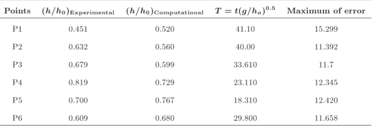
The locations of stations P1, P2, P3, P4, P5, and P6 are shown in Figure 4. Dimensionless level of water over time is compared with experimental data at these points. This comparison is displayed in Figure 5. The plots are depicted for 9.5 seconds.
After the sudden removal of the gate, a decline and a rise in water level may occur for P1 and P2, respectively, up to T = 5. From T = 5 to T = 40, the water level changes a little at these points. After the passing and reection of water wave of the bump (T = 40), the water level declines gradually at P1 and P2. When the wave front reaches P3, the water level increases suddenly. The duration of the water level being constant (T = 20 29) is shorter for P3 than that for P1 and P2. At P4, P5, and P6, the water level grows without being constant. The free surface ow changes a little behind the negative wave. At this time, the ow transmutes into the subcritical ow via hydraulic jump and, then, passes the bump. In this stage, the water levels remain constant in maximum values, because inow and outow are in balance. At
Table 1. Maximum of error calculated at dierent dimensionless times shown in Figure 3. T = t(g=ho)0:5 (h=h0)Experimental (h=h0)Computational x=h0 Maximum of error
15.16 0.619 0.640 7.621 3.39
17.54 0.163 0.190 12.310 14.210
20.67 0.507 0.558 6.130 10.059
23.05 0.790 0.838 6.731 6.075
29.69 0.610 0.541 3.490 11.311
35.83 0.520 0.580 1.411 11.538
41.84 0.325 0.290 9.320 10.769
49.99 0.574 0.540 0.747 5.923
Figure 4. The location of measurement stations.
T > 40, the water level declines in downstream, while negative wave moves to the upstream. In general, the good agreement exists between results of the present model and the experimental data.
5.1.6. Calculation of relative error
As for Section 5.1.6, the relative error is calculated using Eq. (26). Therefore, the result is shown in Table 2.
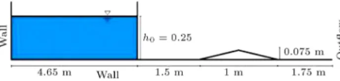
5.2. Wet bed after obstacle with closed end In this case, the experimental data of Soares Frazao et al. [27] are selected for comparison. Initial domain and
dimensions are shown in Figure 6. There is a closed-end boundary condition, and the bed is dry before the bump and wet after it.
5.2.1. Qualitative description of the ow
The ow is described at t = 1:8 s, t = 3:0 s, t = 3:7 s, and t = 8:4 s; images are shown in Figure 7.
When the gate opens, the ows move to the downstream. After the water reaches the obstacle, part of the wave crosses the bump, but another part reects and moves to the upstream. After crossing the bump, the ow reaches the pool of water. At this time (t = 3:0 s), a positive front wave forms and travels to
Table 2. Maximum of error calculated for points specied in Figure 5.
Points (h=h0)Experimental (h=h0)Computational T = t(g=ho)0:5 Maximum of error
P1 0.451 0.520 41.10 15.299
P2 0.632 0.560 40.00 11.392
P3 0.679 0.599 33.610 11.7
P4 0.819 0.729 23.110 12.345
P5 0.700 0.767 18.310 12.420
Figure 5. Comparison of the water level between the present model results and the experimental data of Ozmen-Cagatay et al. [26] for time evolution at dimensionless distance: (a) X = 0:6, (b) X = 0:6, (c) X = 3, (d) X = 6, (e) X = 7, and (f) X = 8.
the upstream. Then, this ow moves to the bed and reaches the bump and is reected again (t = 3:7). At t = 8:4 s, the water on the bump is balanced.
5.2.2. Comparison of the free surface prole with the experimental data
In this section, a comparison of the free surface prole with the experimental data is carried out. Then, the results are shown in Figure 8 at t = 1:8 s, t = 3:0 s, t = 3:7 s, and t = 8:4 s. In these times, the present model reproduces good results.
Figure 6. Initial geometry of bumpy channel with wet bed after obstacle [27].
Figure 7. Free surface prole and comparison between the present model results and the experimental data of Soares Frazao et al. [27] at dierent times for a channel with wet bed after the obstacle.
Table 3. Maximum of error calculated at dierent times shown in Figure 8. t (s) ZExperimental (m) ZComputational (m) X (m) Maximum of error
1.8 0.022 0.025 4.912 13.636
3.0 0.048 0.054 5.130 12.50
3.7 0.082 0.069 3.87 14.606
8.4 0.067 0.059 3.63 11.940
Figure 8. Comparison of water surface proles between the present model results and the experimental data of Soares Frazao et al. [27] at dierent times.
5.2.3. Calculation of relative error
The calculation of error is the same as in section 5.1.4 and 5.1.5 which is given in Table 3.
5.3. Rectangular obstacle
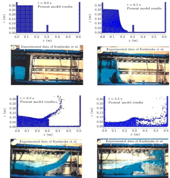
In this section, the liquid behavior, when facing the rectangular obstacle, is investigated and compared with that in the experimental data of Koshizuka et al. [28]. The initial geometry of this case is provided in Figure 9. This gure illustrates the experimental data and the numerical results at t = 0:1, 0.2, 0.3, and 0.5 s; the results of the numerical model are slightly dierent from those of the experimental data, since air fazing is neglected in the numerical model. The good agreement exists between the experimental data and the numerical results.
6. Discussions
In the previous sections, the ood waves in the channel with the dierent boundary conditions were
investi-gated. Case one was a channel with dry bed and open end. Dam break problem was studied in this channel. Then, the free surface prole was compared with the experimental data of Ozmen-Cagatay et al. [26]. The results of this model were in very good agreement with those of the experimental data. Therefore, the maximum of relative error was calculated for dierent dimensionless times, showing good accuracy of the numerical model. The second case was the channel with the closed end and the bed after the obstacle was considered wet. Then dam break waves were investigated for this case. This problem was compared with the experimental data of Soares Frazao et al. [27]. At the end of this part, the maximum of relative error was computed for dierent times. Through the analysis of the results and maximum of error, it can be found that the results of the present model have good eciency for modeling the interference of waves. In the third case, a channel with a rectangular obstacle was considered. For this example, the results of the present model are compared with the experimental data of Kushizuka et al. [25]. For this case, ow of dam break had acceptable accordance with the experimental data. 7. Conclusion
In this paper, a numerical modelling of ood waves in a bumpy channel with dierent boundary conditions was developed. An ISPH Method was presented to simulate ood waves in a bumpy channel with dierent boundary conditions. SPH is a Lagrangian particle method that does not require a grid to simulate free surface ows. Wave breaking is one of the phenomena whose free surface is complicated. Therefore, particle methods, such as ISPH method, represent a robust tool for the modelling of this kind of free surface. The method employs particles to discretize the Navier-Stokes equations, and the interactions among particles simulate the ows. Thus, the advection terms in Navier-Stocks equations were calculated directly, thus omitting numerical diusion errors. In the present model, a new technique was applied to determine den-sity of the particles for the calculations. By employing this technique, ISPH method became stable. The numerical validation and verication were performed through experimental data to prove the capability of
Figure 9. Free surface prole and comparison between the present model results and the experimental data of Kushizuka et al. [28] at dierent times for a channel with a rectangular obstacle.
the ISPH model to simulate ood waves interaction in uneven beds with various boundary conditions. Therefore, the results showed that the free surface ows in the channels with dierent boundary conditions were simulated using ISPH method with high accuracy. On the other side, the computed relative error indicates this fact, too.
References
1. Ataie-Ashtiani, B., Shobeiry, G., and Farhadi, L. \Modied incompressible SPH method for simulating free surface problems", Fluid Dynamic Research, 40, pp. 637-661 (2008).
2. Stoker, J.J., Water Waves. Pure and Applied Mathe-matics 4, Interscience Publishers, New York (1957). 3. Xia, J., Lin, B., Falconer, R.A., and Wang, G.
\Modelling dam-break ows over mobile beds using a 2D coupled approach", Adv. Water Resour., 33(2), pp. 171-183 (2010).
4. Shakibaeinia, A. and Jin, Y.C. \A mesh-free particle model for simulation of mobile-bed dam break", Adv. Water Resour., 34(6), 794-807 (2011)
5. Harlow, F. and Welch, J. \Numerical calculation of time-dependent viscous incompressible ow of uid with free surface", The Physics of Fluids, 8(12), pp. 2182-2189 (1965).
6. Hirt, C.W. and Nichols, B.D. \Volume of uid (VOF) method for the dynamics of free boundaries", Journal of Computational Physics, 39, pp. 201-225 (1981). 7. Khanpour, M., Zarrati, A.R., and Kolahdoozan, M.
\Numerical simulation of the ow under sluice gates by SPH model", Sharif University of Technology, Scientia Iranica, Transactions A: Civil Engineering, 21(5), pp. 1503-1514 (2014).
8. Shao, S.E. and Lo, E. \Incompressible SPH method for simulating Newtonian and non-Newtonian ows with a free surface", Advances in Water Resources, 26, pp. 787-800 (2003).
Ch. \Improved SPH method for simulating free surface ows of viscous uids", Applied Numerical Mathemat-ics, 59, pp. 251-271 (2009).
10. Wang, B.L. and Liu, H. \Application of SPH method on free surface ows on GPU", Journal of Hydrody-namics, 22(5), pp. 912-914 (2010).
11. Lee, E.S., Xu, C., Moulinec, R., Violeau, D., Laurence, D., and Stansby, P. \Comparisons of weakly compress-ible and truly incompresscompress-ible algorithms for the SPH mesh free particle method", Journal of Computational Physics, 227, pp. 8417-8436 (2008).
12. Khayyer, A. and Gotoh, H. \On particle-based simu-lation of a dam break over a wet bed", J. Hydraul. 595 Res., 48(2), pp. 238-49 (2010).
13. Ozbulut, M., Yildiz, M., and Goren, O. \A numerical investigation into the correction algorithms for SPH method in modeling violent free surface ows", Journal of Mechanical Sciences, 79, pp. 56-65 (2014).
14. Monaghan, J.J. \Simulating free surface ows with SPH", Journal of Computational Physics, 110, pp. 399-406 (1994).
15. Morris, J.P., Fox, P.J., and Zhu, Y. \Modeling low Reynolds number incompressible ows using SPH", Journal of Computational Physics, 136, pp. 214-226 (1997).
16. Chorin, A.J. \Numerical solution of the Navier-Stokes equations", Mathematics of Computation, 22, pp. 745-762 (1968).
17. Cummins, S.J. and Rudman, M." An SPH projection method", Journal of Computational Physics, 152, pp. 584-607 (1999).
18. Shao, S. and Gotoh, H. \Simulating coupled motion of progressive wave and oating curtain wall by SPH-LES model", Coastal Engineering Journal, 46, pp. 171-202 (2004).
19. Hu, X.Y. and Adams, N.A. \An incompressible multi-phase SPH method", Journal of Computational Physics, 227, pp. 264-278 (2007).
20. Xenakis, A.M., Lind, S.J., Stansby, P.K., and Rogers, B.D. \An incompressible SPH scheme with improved pressure predictions for free-surface generalized New-tonian ows", Journal of Non-NewNew-tonian Fluid Me-chanics, 218, pp. 1-15 (2015).
21. Nomeritae, Daly, E., Grimaldi, S., and Hong Bui, Ha. \Explicite incompressible SPH algorithm for free-surface modeling: A comparison with weakly com-pressible schemes", Advances in Water Resources, 97, pp. 156-167 (2016).
22. Dalrymple, R.A. and Rogers, B.D. \Numerical mod-eling of water waves with the SPH method", Coastal Engineering Journal, 53, pp. 141-147 (2006).
23. Monaghan, J.J. \Smoothed particle hydrodynamics", Annu RevAstron Astrophys, 30, pp. 543-57 (1992).
24. Shao, S. \Incompressible SPH ow model for wave interactions with porous media", Coastal Engineering Journal, 57, pp. 304-316 (2010).
25. Koshizuka, S. and Oka, Y. \Moving-particle semi-implicit method for fragmentation of incompressible uid", Nuclear Science and Engineering, 123, pp. 421-434 (1996).
26. Ozmen-Cagatay, H., Kocaman, S., and Guzel, H. \Investigation of dam-break ood waves in a dry channel with a hump", Journal of Hydro-environment Research, pp. 1-12 (2014).
27. Soarez Frazao, S., de Bueger, C., Dourson, V., and Zech, Y. \Dam-break wave over a triangular bottom sill", International Conference on Fluvial Hydraulics, pp. 437-442 (2002).
28. Koshizuka, S., Oka, Y., and Tamako, H. \A particle method for calculating splashing of incompressible viscous uid", Int. Conf. Math. Comput., 2, pp. 1514-1521 (1995).
Biographies
Sajedeh Farmani received BSc degree in Civil En-gineering and MSc degree (with rst rank) in Hy-draulic Engineering from Shahid Bahonar University of Kerman, Iran in 2012 and 2014 respectively. Now, she is a PhD Student in Civil Engineering (hydraulic structures) in the same university. She published more than 6 papers in international journals and conferences. Her research interests include numerical simula-tion, dam-break ow, SPH method, numerical mod-eling of tuned liquid dampers, FEM method in free surface ow, and improvement of nite-element method in modeling of uid mechanics.
Gholam-Abbas Barani graduated from UC Davis at California, USA in 1981. His eld of interest is Water Resource Engineering, studying at the Civil Engineering Faculty of Shahid Bahonar University, Kerman since 1981. Currently, he is a Professor. His academic activities include teaching hydraulics, ad-vanced hydraulics, hydraulic structure, and adad-vanced groundwater for BS, MSc, and PhD programs as well as publishing about 53 papers in international and national journals and presenting and publishing more than 200 paper in national and international conferences.
Mahnaz Ghaeini-Hessaroeyeh received her PhD degree in Civil Engineering (Water Engineering) from Amirkabir University of Technology in 2010. She has been as an Assistant Professor at the Civil Department of Shahid Bahonar University of Kerman since 2011 up until now.
Her research interests include computational uid dynamics, sediment transport modeling, supercritical
ow over hydraulic structures, dam-break ow over movable beds, and numerical modeling of ground water ow. She has contributed/presented more than 75 pa-pers in various journals and national and international conferences.
Rasoul Memarzadeh received the BSc degree in Civil Engineering from Vali-e-Asr University of Raf-sanjan, Iran in 2009. Then, he continued his studies and researches in the elds of Water and Hydraulic engineering. He received MSc degree in Civil
(hy-draulic) Engineering from the Khaje Nasirodin Toosi University of Technology, Tehran, Iran in 2012 (with rst rank), and PhD degree in the same eld from the Shahid Bahonar University of Kerman, Iran in 2017 (with rst rank). He published more than 15 papers in international journals and conferences. His current research interests include hydraulic engineering, uid mechanics, numerical simulation, computational uid mechanics (CFD), meshless methods, SPH method, waves and currents, multi-phase ows, and sediment transport.

![Figure 6. Initial geometry of bumpy channel with wet bed after obstacle [27].](https://thumb-us.123doks.com/thumbv2/123dok_us/8370311.2223053/7.892.86.438.147.850/figure-initial-geometry-bumpy-channel-wet-bed-obstacle.webp)