1244.pdf

(1)

11

MING-MING CHEN. Computational Simulation of worker exposure Using a Particle Trajectory Method. ( Under the direction of Dr. Michael R. Flynn)

ABSTRACT

A discrete vortex model of the recirculating flow downstream of a worker is used to calculate trajectories of "massless" tracer particles released from a fixed point source. Mean concentrations in the plane of the source are estimated by averaging over a number of such trajectories. Approximations include: (1) the worker is represented by a two-dimensional elliptical cylinder; and (2) the contaminant is represented by massless tracer particles which are

generated without momentum and transported by vortex shedding and turbulent diffusion exclusively. Computer-predicted mean

(2)

Ill

TABLE OF CONTENTS

Page

TABLE OF CONTENTS... iii

LIST OF TABLES AND HGURES... i v ACKNOWLEDGEMENTS... vii

INTRODUCTION... 1

CALCULATION METHOD... 4

(a) Trajectories... 4

(b) Mean Concentrations... 7

RESULTS... 1 1 DISCUSSION... 2 3

CONCLUSIONS... 2 7

REFERENCES...'... 2 8

APPENDIX A:

Determination of Eddy Diffusivity ke... 3 0

APPENDIX B:

The Relation Between the Weighting Factor, f(t), and

the Lagrangian Integral Time-Scale, Tl... 3 2

APPENDIX C:

(3)

IV

LIST OF TABLES AND FIGURES

Page

TABLE 1

Summary of the Trajectory Algorithm of the Concentration

Particles... 7

TABLE 2

The Average Concentration from the 28 Examining Points

for Each Simulation and Experiment... 1 3 FIGURE 1

Plan View of Worker and Point-Source Relative Positions... 2

FIGURE 2

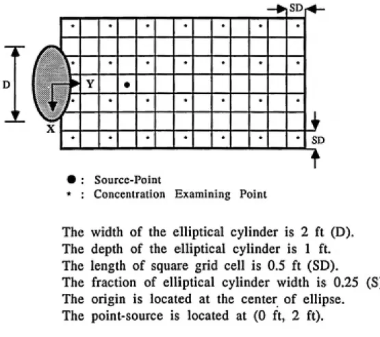
The Dimensions of the Grid Cells in the Plane of Point-Source 3

FIGURE 3

The Total Number of Particles Generated in Two-Dimensional

Concentration Field... 1 4

FIGURE 4

The Average Number of Weighted Particles in the Cell of

the Point-Source... 1 5

FIGURES

The Average Number of Weighted Particles in the area

(4)

FIGURE 6

The Concentration Contours for Point-Source at (0 ft, 2 ft)

with ke=0.074, Tl=0.58... 1 7

FIGURE?

with ke=0.74, Tl=0.58... 1 8

FIGURES

withke=7.4, Tl=0.58... 1 9

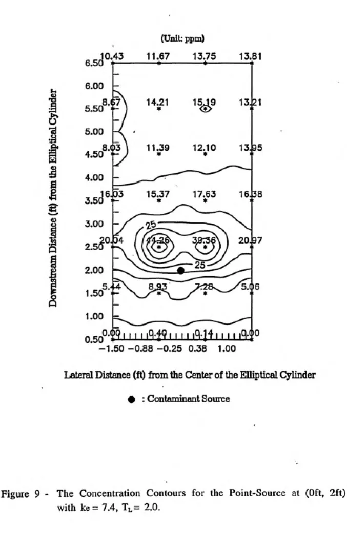
FIGURE 9

with ke=7.4, Tl=2.0... 2 0

FIGURE 10

with ke=74., Tl=10.0... 2 1

FIGURE 11

The Concentration Contours of Experiment... 2 2 FIGURE 12

Air Flow Structure Downstream of the Mannequin... 2 5

FIGURE 13

Velocity Field around an Elliptical Cylinder in a Uniform

(5)

VI

FIGURE B.l

Particle Variances in Z-Direction, ^z, with Different Tl

Values... 3 3

FIGURE B.2

(6)

Vll

ACKNOWLEDGEMENTS

I wish to express my thanks to my advisor. Dr. Michael R. Flynn, for his knowledge and guidance throughout this research; to Dr.

(7)

INTRODUCTION

In a paper entitled 'Discrete vortex methods for the simulation

of boundary layer separation effects on worker exposure', Flynn and

Miller (1991) point out that one of the most significant aspects of

contaminant dispersion in the vicinity of a worker is the tendency

for the contaminant to recirculate. The phenomenon of boundary

layer separation is responsible for the formation of rotating eddies

on the downstream side of the worker. These eddies can transport

contaminant into the breathing zone and reduce the effectiveness of

the intended ventilation (Flynn and Miller, 1991).

The objective of this research is to develop a computer model

to calculate trajectories of particles released from a fixed

point-source in a two-dimensional flow field and to estimate mean

concentrations in the plane of this source. The model represents the

worker as an elliptical cylinder. The time-dependent air flow is

around this elliptical cylinder which is immersed in a uniform free

stream (see Figure 1). The recirculating flow downstream of the

worker is computed with a discrete vortex code developed by Flynn

and Miller (1991) and a fast-multipole algorithm developed by

Greengard and Rokhlin (1987) for calculating vortex interactions.

The dispersion of contaminant from a point-source is examined

by calculating trajectories for a number of particles released into the

flow field. Mean concentrations are predicted by imposing a uniform

grid of cells on the wake region (see Figure 2) and counting the

average number of particles in each grid cell. This two-dimensional

(8)

point-source by using a time-dependent particle weighting factor

(Turfus, 1988). A comparison between the mean concentrations

computed from the simulation and those measured using a

mannequin and sulfur hexafluoride (SFg) tracer gas (Flynn and Kim,

1990), is conducted to examine the model's validity.

Wall

Tunnel

Inlet

I--- Elliptical Cylinder (represents worker)

Concentration Area

r

i

— Contaminant Source

U (Freestream Velocity)

Removal Boundary

(for Concentration Particles)

Tunnel Outlet

Wall

(9)

D

-

ͨ

]

SD

r4-* * * * * * *

1*^

T

Y

* * * ͣk * •

J^

Y •

/

* * • * * *

X

il

* * * * * * ͣk

SD

• : Source-Point

* : Concentration Examining Point

The width of the elliptical cylinder is 2 ft (D). The depth of the elliptical cylinder is 1 ft.

The length of square grid cell is 0.5 ft (SD).

The fraction of elliptical cylinder width is 0.25 (S). The origin is located at the center of ellipse.

The point-source is located at (0 ft, 2 ft).

(10)

CALCULATION METHOD

(a) Trajectories

Airflow around an elliptical cylinder is time-dependent;

entrainment of air into the near-wake region results in the periodic

shedding of vortices. It is assumed that this determines the

concentration of contaminant to which the worker is exposed.

Trajectories for passive tracer particles released from a given point

source in this two-dimensional flow field, are calculated using a

discrete vortex model (Flynn and Miller, 1991). This model relies

upon the fact that vorticity is a material property of the fluid that is

convected and diffused. It is possible to use the method of fractional

steps (Bui and Oppenheim, 1987) and split the vorticity-transport

equation into Euler's equation and the diffusion equation,

respectively:

-^ + (V- V)^ = 0

at '^ (1)

and

at ^, (2)

where ^ is vorticity, V is the two-dimensional velocity, and v is the

kinematic viscosity.

The solution for Euler's equation depends upon a theorem

(Batchelor, 1967) that guarantees, for an incompressible flow, that a

(11)

diffusion equation, with an impulse initial condition, is a Gaussian

distribution of zero mean and variance:

2

a- = 2v At, (3)

where a is the standard deviation of a blob or sheet displacement

and At is a finite interval of time.

Under the assumption that the small scale contaminant

diffusivity, ke is a constant, then the contaminant-transport equation

can be split into Euler's equation and the diffusion equation,

respectively:

3C

—- + (V • V) C = 0

at (4)

and

^t , (5)

where C is the concentration of the contaminant, V is the two-dimensional velocity, and ke is the diffusivity.

Concentration particles are treated as massless tracer particles

that are generated without momentum. In simulation, the movement

of the concentration particle is affected by the convection of vortex

blobs and the diffusion of eddies in the flow field. The movements of

the concentration particles are according to the equations:

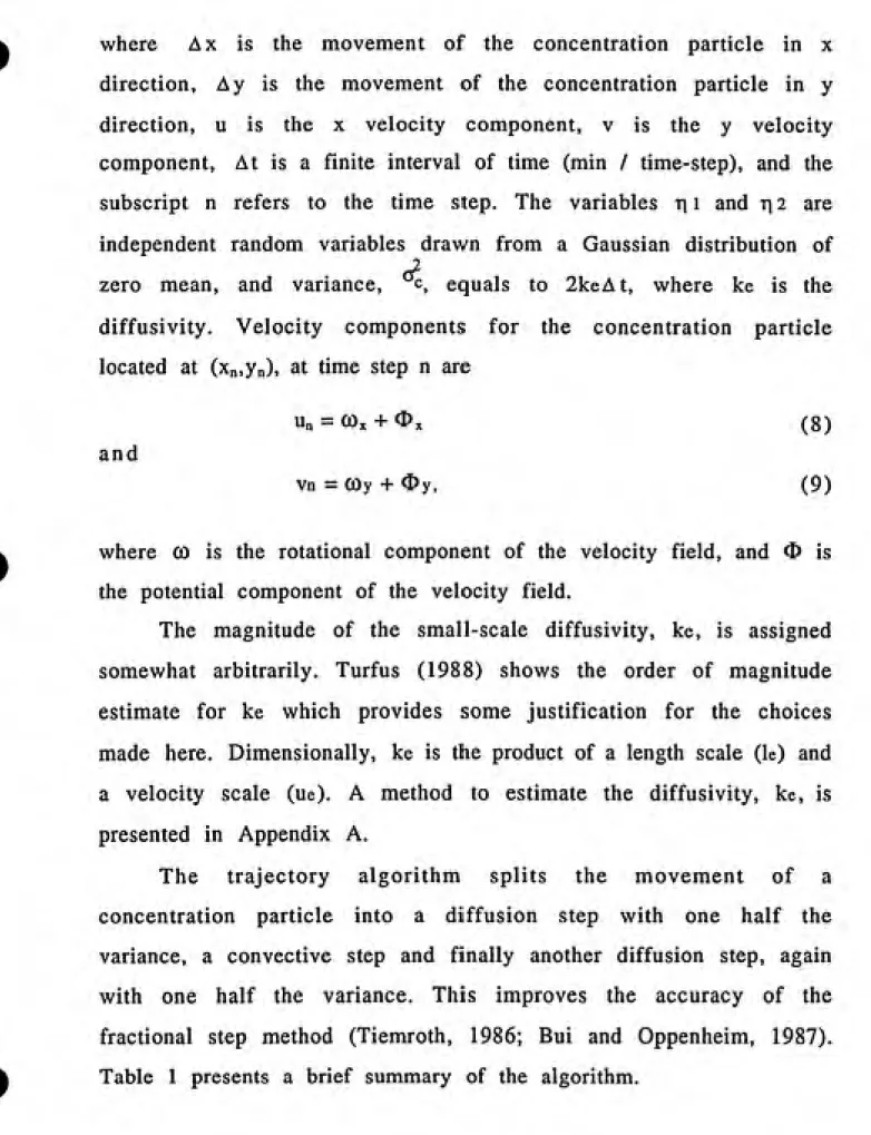
Ax = Xn+, - x„ = At u„ + rii (6) and

(12)

where Ax is the movement of the concentration particle in x

direction, Ay is the movement of the concentration particle in y

direction, u is the x velocity component, v is the y velocity

component. At is a finite interval of time (min / time-step), and the

subscript n refers to the time step. The variables r| i and ri 2 are

independent random variables drawn from a Gaussian distribution of

J.

zero mean, and variance, c, equals to 2keAt, where ke is the

diffusivity. Velocity components for the concentration particle

located at (Xn,yn), at time step n are

u„ = C0x + O^ (8)

and

Vn = COy + Oy, (9)

where CO is the rotational component of the velocity field, and O is

the potential component of the velocity field.

The magnitude of the small-scale diffusivity, ke, is assigned

somewhat arbitrarily. Turfus (1988) shows the order of magnitude

estimate for ke which provides some justification for the choices

made here. Dimensionally, ke is the product of a length scale (le) and

a velocity scale (ue). A method to estimate the diffusivity, ke, is

presented in Appendix A.

The trajectory algorithm splits the movement of a

concentration particle into a diffusion step with one half the

variance, a convective step and finally another diffusion step, again

with one half the variance. This improves the accuracy of the

fractional step method (Tiemroth, 1986; Bui and Oppenheim, 1987).

(13)

TABLE 1

Summary of the Trajectory Algorithm for the Concentration Particles

Within each time step:

(1) Generate the new concentration particles at the source point.

(2) Diffuse all old concentration particles.

(3) Reflect and / or remove the concentration particles from

domain as needed.

(4) Convect all old concentration particles.

(5) Reflect and / or remove the concentration particles from

domain as needed.

(6) Diffuse all old concentration particles.

(7) Reflect and / or remove the concentration particles from

domain as needed.

(b) Mean Concentrations

The main purpose of this research is to predict mean

concentrations resulting from a constant generation rate of

contaminant from a fixed point-source. After the flow field develops,

concentration particles are released, ten particles per time-step, from

a fixed point source. They are allowed to move under the influence of

the flow field, according to Equations (4) and (5). These particles are

removed only when they cross the removal boundary (RB). RB is

y=18 ft, that was tested and set in simulation, because beyond this

boundary the probability of particle being recirculated back to the

wake region is zero. After a given time, the distribution of particles

in the flow reaches a statistical equilibrium, i.e. the expected number

(14)

increase or decrease with time. By the ergodic theorem (Panchev,

1971), if the distribution of particles were statistically stationary

throughout this time period and the average number of particles in

each cell at each time-step had therefore converged to a number

independent of time, then we could equate this number to the

ensemble mean concentration (due to a line-source of strength Qs = N

particles /At) integrated over the cell.

Turfus (1988) presents a method for estimating concentration

from point and line sources in a two-dimensional flow. For a

line-source, the mean concentration, C, can be expressed as a

dimensionless group % by the following transform:

CILD

X(xi,yj)= ^°° ao)

where U~ is the freestream velocity (fpm), Qs is the two-dimensional

source strength (ft2 /min), and D is the width of the mannequin (ft)

which is perpendicular to the free stream.

By imposing a uniform grid over the computational domain

with square cells of length SD, if Ny is the calculated mean number of

particles in a cell with center at (Xi, yj), then the dimensionless mean

concentration within this cell can be approximated as:

NijU^DAt NijU^At

X Xi, yj) = / .— = -7^-^^— a 1)

(SD) N (s^d) N

where S is a fraction of length D, and N is the number of particles

(15)

A similar analysis is presented by Turfus (1988) for calculating

concentration fields in the plane of a point-source, in a

two-dimensional flow, by including a weighting factor inversely

proportional to the age of the particle (i.e. the time since the particle

is released). Thus, the dimensionless mean concentration for a

point-source, X3D, is defined as:

O(xi,yj,z=0) U^D^

X3D(xi, yj) = —---^-^--- a^

where Qs is the contaminant source flow in cfm. Equation (9) can be

modified as:

N*ij U^ At

*

where "^ '' is the number of weighted tracer particles in the ij cell.

Equation (13) is used to approximate the concentration field in the

plane of the point source by weighting the contribution of each

particle with a factor, f(t), where:

f(t) = -1---=--- a 4)

^2k G^it)

and

(4(t) = 5^ -h 2(4 1? a - e T^ -H ^) a 5)

where ^ is the particle variance in z direction, t is the age of the

(16)

10

a small distance to avoid singularity in the formlation, and *^ is the

velocity variance out of the plane of simulation (i.e. the square of the

z-velocity fluctuation). Based on homogeneity, "w is calculated

assuming a 10% overall turbulence intensity.

Turfus (1988) examined the recirculation bubble downstream

of a backward facing step and concluded a dimensional simulation

time of Td = 144 D (U~>)" had a 10% error. Based upon similar

reasoning for our research if D is the mannequin cross body

dimension of 8 inches, U- is 200 fpm, and At is 0.002 min; then 240

(17)

RESULTS

The simulations conducted here represent flow of air around a

worker by modelling this worker as a two-dimensional elliptical

cyclinder. The cylinder is 2.0 ft wide, and 1.0 ft deep. The free

stream velocity was set to 66.67 fpm, with the direction of air flow

perpendicular to the major axis, thus giving a Reynolds number of

13890, in the range applicable to industrial ventilation.

A time increment of 0.002 min was selected for the runs

displayed here. After 150 time steps (i.e. the time needed to develop

the velocity flow field), concentration particles were released, 10

particles per time step, from a point-source into the two-dimensional

flow field. The time needed for the concentration field to reach

statistical equilibrium, after the particles are introduced into the flow

field, is presented in Figure 3. This shows the development of

concentration particles with time in the region -7.5 ft < x < 7.5 ft and

0 ft < y < 18 ft. It indicates that after about 200 time steps, the

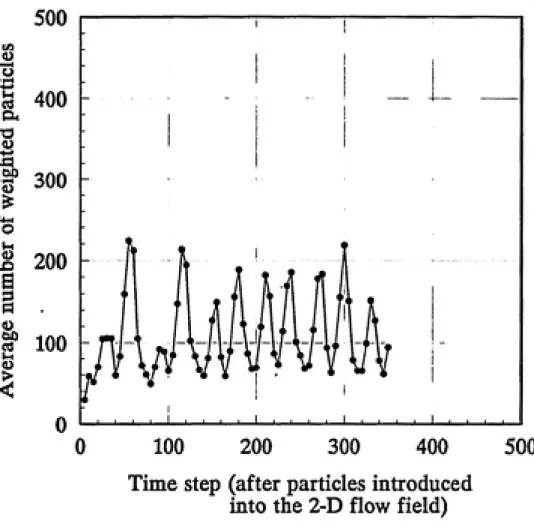
distribution of particles in the flow reaches equilibrium. Figure 4 and

Figure 5 show the distributions of weighted particles with time in the

cell of the point-source and in the area -1.25 ft < x < 1.25 ft and 0.75

ft< y < 3.25 ft, respectively. These show that the equilibrium state can

be reached quickly in the area close to the cylinder. The calculation

was continued for 100 time steps to calculate the mean

concentrations of examining points in the wake region.

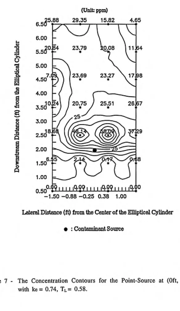
Mean concentration contours resulting from a point-source

located at (0.0 ft, 2.0 ft) were calculated. Figures 6-8 present the

(18)

12

ke=0.74, and ke=7.4 and Tl=0.58, respectively. It shows mean

concentrations near the worker increase when the diffusivity

increases. Results for mean concentration contours with Tl=2.0, and

Tl = 10.0 and ke=7.4 are presented in Figure 9 and Figure 10,

respectively. The mean concentration contours of experimental data

are presented in Figure 11 (Flynn and Kim, 1990). Table 2 presents

the average concentration from the 28 examining points for each

simulation and experiment. It shows that the mean concentration

decreases when either the diffusivity (ke) or the Lagrangian integral

time scale (Tl) increases.

The simulations displayed here adopt a fast-multipole

algorithm developed by Greengard and Rokhlin (1987) which

reduces computational time from order N^ to order N (where N is the

(19)

TABLE 2

The Average Concentration from the 28 Examining Points

for Each Simulation and Experiment

13

Case Diffusivity ke

Lagrangian integral

time scale, Tl

Average mean 1

concentration (ppm) 1

1 0.074 0.58 17.40

2 0.74 0.58 17.10

3 7.4 0.58

14.16 1

4 7.4 2.00 12.98

5 7.4 10.0 7.89

(20)

14

ex

o

2000

1600 Q

(^

.S

I 1200

800

^ 400

0

0 100 200 300 400 500

Time step (after particles introduced

into the 2-D flow field)

Figure 3 - The Total Number of Particles Generated in Two-Dimensional

(21)

15

xi

cd 100

80

S 60

40

20

-0

0 100 200 300 400 500

Time step (after particles introduced

into the 2-D flow field)

Figure 4 - The Average Number of Weighted Particles in the Cell of

(22)

16

4>

500

J3 400

Oh

ͣ

«-»

t 300

I 200

I .

I 100

0

0 100 200 300 400 500

Time step (after particles introduced

into the 2-D flow field)

Figure 5 - The Average Number of Weighted Particles in the Area of

(23)

17

I

!

I

6.50

(Unit: ppm)

33.79 36.21

T7.ZQ

o.coQ-t?...^^ Mil iq-?91111 iM-yo

-1.50-0.88-0.25 0.38 1.00

Lateral Distance (ft) from the Center of the EUipticad Cylinder

Contaminant Source

Figure 6 - The Concentration Contours for the Point-Source at (Oft, 2ft)

(24)

18

.^5.88

(Unit: ppm) 29.35 15.82

23.79

o.3oQ19...q-;9...q>y9 mm iq-f

-1.50-0.88-0.25 0.38 1.00

Lateral Distance (ft) from the Center of the Elliptical Cylinder

: Contaminant Soinx:e

Figure 7 - The Concentration Contours for the Point-Source at (Oft, 2ft)

(25)

19

e cJ 0.59

6.50

(Unit: ppm)

15.25 13.75

11.66

-1.50-0.88-0.25 0.38 1.00

: Contaminant Source

Figure 8 - The Concentration Contours for the Point-Source at (Oft, 2ft)

(26)

20 ti4

I

u •a a Q 6.50 6.00 5.50_8.()7 5.00 4.50 8.03 (Unit: ppm) 11.67 ---iti— 14.21 11.39 * 13.75 —*— 15J9 12.10 13.81 —* 13.21 13.95

15.37 _{17.63 16J38}

20.97

5.06

0.500-f9...q-t^? MM lQ^l,-^ I I I I iQ-f

-1.50-0.88-0.25 0.38 1.00

Figure 9 - The Concentration Contours for the Point-Source at (Oft, 2ft)

(27)

21

(Unit: ppm)

4.05 5.50

-0.50

iiiiiiq>f?iiiiiqvl7MMiq-f5

-1.50-0.88-0.25 0.38 1.00

•: Contaniinant Source

Figure 10 - The Concentration Contours for the Point-Source at (Oft, 2ft)

(28)

22

(Unit: ppm)

S

0.50

1.97

1.50 "t

-J

-1.50-0.88-0.25 0.38 1.00

Lateral Distance (ft) from the Center of the Mannequin

Figure 11 - The Concentration Contours of Experiment (Flynn and Kim,

(29)

DISCUSSION

Mean concentrations predicted in a two-dimensional flow field by using the particle trajectory algorithm, are determined by three major factors: (1) the recirculation, which is caused by vortices in the

flow; (2) the diffusivity, ke, which tends to spread the contaminant

particles away from the point-source; and (3) the weighting factor, f(t), which determines the probabilities of contaminant particles

leaving the source plane.

Mean concentrations are computed by selecting different values of diffusivity (ke) from 0.074 to 7.4 in our simulations. For ke = 0.074 and ke = 0.74, there is no concentration predicted at level

y=0.5 ft. Figures 6-8 show that for the smaller ke the spread of contaminant away from the source is slower. Because the average velocity of the flow in the wake region is difficult to be determined. It is difficult to obtain an accurate eddy diffusivity for a given simulation, but there is a method presented in Appendix A for

estimating the value of ke. The particle weighting factor which is a

function of the age of particle is affected by the Lagrangian integral

time scale (see Appendix B). Tl is considered a measure of the longest

time during which a particle persists in a motion in a given direction (Hinze, 1975). Figure 9 and Figure 10 show that the larger Tl selected the lower mean concentrations are predicted in the plane of the

source. Table 2 shows that there is no significant difference between

the mean concentrations of the examining area by selecting values of

(30)

24

selects values of Tl from 0.58 to 10.0. This indicates that mean concentrations are more strongly affected by Tl than ke.

Generally, the pattern of mean concentration contours

predicted agrees with that of experimental measurement. By

comparing concentrations predicted from simulations with those measured from experiment, the main differences are: (1) computations underpredict mean concentrations near the wake

region, but overpredict concentrations downstream of the

point-source; and (2) for computations, the highest mean concentration

area is at the downstream side of point-source which is different

from experimental where the peak occurred at the upstream side of

the point-source. These discrepancies may be due to: (1) the effect of

the mannequin's elbows, which keeps contaminant in the near wake

region; and (2) the effect of the vertical recirculating loop, which

recirculates the contaminant back to the near wake region (Kim and Flynn, 1991). Mean concentrations in the plane of the point-source are strongly affected by the vertical recirculating loop coming down from the mannequin's head in experiment (see Figure 12). This not

only disperses the contaminant out of the plane of the point-source

but also recirculates it back to the near wake region.

A skewness of the free stream toward the cylinder in the

two-dimensional velocity field was observed (see Figure 13). The effect resulting from the skewness in velocity field is still not clear, but we know that the direction of this velocity skewness is changed with time and is related to eddies formed downstream of the cylinder.

This phenomenon will be reconsidered subsequently to improve the

(31)

25

Plan View

Side View

Figure 12 - Air Flow Structure Downstream of the Mannequin (Kim and

(32)

26

K

/V/ Wk

\AA

M^

-2.00-1.00 0.00

(33)

CONCLUSION

It is important to develop a computational model for predicting worker exposure. If the worker's breathing zone concentration can be estimated before control equipment be installed, then the design of a local exhaust ventilation system can be evaluated prior to its construction. The extra cost of over control can be eliminated and the

optimal design implemented to control worker exposure to hazardous airborne pollutants. It is difficult to use a two-dimensional computational model to simulate the flow from the vertical recirculating loop and predict the three-dimensional exposure of worker. The particle trajectory algorithm provides a good research direction for the three-dimensional simulation of the mean

(34)

28

REFERENCES

Batchelor, G.K. : An Introduction to Fluid Dynamics. Cambridge University Press, Cambridge, U.K., 1967.

Bui, T.D. and A.K. Oppenheim: Evaluation of Wind Effects on Mode Buildings by the Random Vortex Method. Appl. Numer. Math. 3,

195-207 (1987).

Flynn, M.R. and T. Kim : The Impact of Separation on Exposure and Hood Capture. The Final Report on NIOSH grant 5 ROl OH 02392-02 (1990).

Flynn, M.R. and C.T. Miller : Discrete Vortex Methods for the

Simulation of Boundary Layer Separation Effects on Worker Exposure. Ann. Occup. Hyg., 35(l):35-50 (1991).

Greengard, L. and V. Rokhlin : The Rapid Evaluation of Potential

Fields in Three Dimensions, in Lecture Notes in Mathematics

-Vortex Methods. Springer-Verlag, Berlin (1987).

Hiller, R. and N.J. Cherry : The Effects of Stream Turbulence on Separation Bubbles. J. Wind Engng Ind. Aerodyn., 8: 49-58

(1981).

Hinze, J.O. : Turbulence Diffusion of Fluid Particles; Lagrangian Correlations, Turbulence 2nd ed., pp. 48-58, 1975.

Kim, T. and M.R. Flynn : Airflow Pattern Around a Worker in a Uniform Freestream. Am. Ind. Hyg. Assoc. J., 52(7):287-296

(1991).

Panchev, S. : Random Function and Turbulence. Pergamon Press,

(35)

29

Tiemroth, E.C. : The Simulation of Viscous Flow Around a Cylinder by the Random Vortex Method. Doctoral Dissertation, University of

California, Berkeley (1986).

Turfus, C. : Calculating mean concentrations for steady sources in recirculating wakes by a particle trajectory method. J. Atmos.

(36)

30

APPENDIX A

Determination of the Eddy Diffusivity, ke:

The magnitude of the small-scale diffusivity, ke, was assigned somewhat arbitrarily. Turfus (1988) shows an order of magnitude calculation for ke which provides some justification for the choices made. Dimensionally, ke is the product of a length scale (le) and a velocity scale (ue). le is a representative length scale for the fluctuations occurring on a scale smaller than the minimum length represented in the DVM. This scale is determined by the cut-off radius for the vortices; so we can suppose le = h / tt , where h is the

length of the vortex sheet (h=0.242121 ft in this study).

In the determination of ue, Turfus supposed that the turbulence at the center of the wake has an energy spectrum E(k),

--- k = fraction of the energy residing in Fourier modes with a wavelength 1 < (2n)/k. He assumes that

"' - J E(k) dk (Al)

(u) 27C/1 e

An estimation of E(k) based on the Kolmogorov similarity

theory is the most acceptable option. Thus,

0.9685

'0.558

^.558^"^

-hk^

^^^ =^ ---7---^---iTTe--- as k ^ oo (A.2)

(37)

where L is the length-scale of turbulence (Hillier and Cherry, 1981).

We estimate L=0.5 D. Then E(k) - 1.2657 k"'" and

31

u.

N'

-|l/2

-i- jE(k) dk

27t/le

1.089 (. ^l/3_le ^% J

,1/3

0.34 (IJ - 0145

Turbulence intensity, TI, can be expressed as:

TI (%) = -^^^ X 100 (%)

u

(A3)

where ^™* '^ ' , and we assume u - U„

For turbulence intensity, Turfus assumes TI=10%.

Thus,

u

TI m

100 (%)

" "lioo,

U^ = 01 U^ - 6.667 fpm

Whence "e = 0-145 (u,„,) = 0145 (01 UJ ^ 0.967 fpm and so,

k^ = u, 1, = 0.967

^h^

yTl J

(38)

32

APPENDIX B

The Relation Between the Weighting Factor, f(t), and the Lagrangian Integral Time-Scale, Tl:

The weighting factor, f(t), applied in our research for using a

two-dimensional model to simulate three-dimensions, is a function of

2

the age of the particle and the particle variance in z-direction, "z.

The particle variance in z-direction is a function of the age of the

particle and the Lagrangian integral time scale, Tl. The Lagrangian

integral time scale can be expressed as:

\ = \^ dx KM (Bl)

where RlCO is the Lagrangian auto-correlation coefficient, and t* is

the time for which ^^^ ) = 0 "Xhe Lagrangian integral time scale is

usually considered a measure of the longest time during which, on the average, a particle persists in a motion in a given direction"

(Hinze, 1975). The relation of particle variance, ^, and particle age

with different values of Tl is presented in Figure B.l. Particle

variance is increased when the value of Tl increases. The weighting factor is inversely proportional to the square root of the particle

variance (see Equation (9) above). Thus, the weighting factor

decreases when Tl increases. The relation of weighting factor and the

(39)

33

c

o

U

-3

N

4>

W

8

u

TL=0.58 TL=2.00 TL=10.0

200 400 600

Age of particle (Time steps)

(40)

34

u

o

o Cm

6C

IS

• mm

0.4-TL=0.58 TL=2.00 TL=10.0

0 200 400 600

Age of particle (Time steps)

(41)

35

APPENDIX C

A FORTRAN Code for Computing Mean Concentrations:

************************************************************** * *

* THIS CODE IS DEVELOPED *

* *

* BY * * *

* MING-MING CHEN *

* *

* JULY 4 , 1992 *

* *

* THIS SUBROUTINE IS DEVELOPED TO CALCULATE THE DIMENSIONLESSAL * * MEAN CONCENTRATIONS IN THE PLANE OF A POINT-SOURCE. *

* *

* - TEN PARTICLES ARE GENERATED PER TIME STEP. * * - PARTICLE IS INTRODUCED AFTER 150 TIME STEPS. *

* - A CONCENTRATION EQUILIBRIUM IS REACHED ABOUT 200 TIME STEPS *

* AFTER PARTICLES ARE INTRODUCED INTO THE FLOW. *

* - TOTAL TIME STEPS OF 500 IS RUN FOR CALCULATING THE *

* CONCENTRATIONS. *

* - THE BOUNDARY SET TO REMOVE PARTICLES FROM CALCULATING *

* DOMAIN IS 18 FT. *

* - TURBULENCE INTENSITY APPLIED HERE IS 10%. * * - THE EDDY DIFFUSIVITY APPLIED HERE IS 7.4. * * - THE LAGRANGIAN INTEGRAL TIME SCALE USED HERE IS 10.0. *

* *

* ͣ *

* WITHIN EACH TIME STEP: *

* *

* 1. GENERATE NEW CONCENTRATION PARTICLES AT THE POINT-SOURCE. *

* 2. DIFFUSE ALL OLD CONCENTRATION PARTICLES. * * 3. REFLECT AND / OR REMOVE PARTICLES FROM CALCULATING DOMAIN *

* AS NEEDED. *

* 4. CONVECT ALL OLD CONCENTRATION PARTICLES. *

* 5. REFLECT AND / OR REMOVE PARTICLES FROM CALCULATING DOMAIN *

* AS NEEDED. *

* 6. DIFFUSE ALL OLD CONCENTRATION PARTICLES. *

* 7. REFLECT AND / OR REMOVE PARTICLES FROM CALCULATING DOMAIN *

* AS NEEDED. *

* *

(42)

36

SUBROUTINE CONC( K )

IMPLICIT REAL*8(A-H,0-Z)

REAL* 8 NBLT

PARAMETER (NCX=9, NCY=15, MAXTS=50000, SX=0.0, SY=2.0) COMMON /SIZE/ MAXEQN

COMMON /BLK/ XE(MAXTS,2),YE(MAXTS,2),SE(MAXTS,2),

* LIND(MAXTS),SEFAC,XC(20),YC(20),UPGP(20),VPGP(20),VXBLBGP(20) * VYBLBGP(20),VT(20),SHTL,CVX,CVY,NBLT,ARC(20),XRHS(21),

* XTS(50),YTS(50),X(50),Y(50),XSTRGP(20),A,B,BR,NEL,UMIN, *UMAX,XSEED,VISC,DELT,N,XLIM,YLIM,IBL

COMMON /CELLS/ INTS,NTS,NCP,NPR,NP,NETS,NCKTS,NCOUNT, * PX(MAXTS,2),PY(MAXTS,2),PA(MAXTS),WPCEL(NCX,NCY), * WPCELS(NCX,NCY),CONKI(NCX,NCY),CELLX(NCX),CELLY(NCY), * YRB,CPKE,CONPPM(NCX,NCY),UAVG,TI

KTS = K-INTS

IF (KTS .EQ. 1) THEN

DO 100 1=1.NP

PX(NCP+I,2)= SX PY(NCP+I,2)= SY PA(NCP+I)= l.DOO 100 CONTINUE WPCELS(5,5)= 1.0D00*NP NCP= NCP+NP ELSE

DO 200 I=1,NCP

PA(I)=PA(I)+1.D00

200 CONTINUE

DO 300 1=1,NP

PX(NCP+I,2)= SX PY(NCP+I,2)= SY PA(NCP+I)= l.DOO 300 CONTINUE NCP=NCP+NP CALL CPDIFF CALL CPMETA CALL CPCONV CALL CPMETA CALL CPDIFF CALL CPMETA

IF (KTS .GT. (NETS-INTS)) THEN CALL CALCON(KTS)

ENDIF

RETURN

(43)

37

************************************************************** * * * THIS SUBROUTINE IS DESIGNED TO DIFFUSE CONCENTRATION PARTICLES. *

* *

**************************************************************

SUBROUTINE CPDIFF

REAL* 8 NBLT

PARAMETER (NCX=9, NCY=15, MAXTS=50000, PI=3.141592654)

COMMON /SIZE/ MAXEQN

* LIND(MAXTS),SEFAC,XC(20),YC(20),UPGP(20),VPGP(20),VXBLBGP(20), * VYBLBGP(20),VT(20),SHTL,CVX,CVY.NBLT,ARC(20),XRHS(21),

* XTS(50),YTS(50),X(50),Y(50),XSTRGP(20),A,B,BR,NEL,UMIN,

* UMAX,XSEED,VISC,DELT,N,XLIM,YLIM,IBL

COMMON /CELLS/ INTS,NTS,NCP,NPR,NP,NETS,NCKTS,NCOUNT, * PX(MAXTS,2),PY(MAXTS,2),PA(MAXTS),WPCEL(NCX,NCY), *WPCELS(NCX,NCY),CONKI(NCX,NCY),CELLX(NCX),CELLY(NCY), * YRB,CPKE,CONPPM(NCX,NCY),UAVG,TI

URMS= (TI/100.0)*UAVG

CPKE= (0.145*URMS)*(SHTL/PI)* 100.0

CPMU= O.ODOO

CPSIG= DSQRT(DELT*CPKE)

DO 100 I=1,NCP-NP PX(I,1)= PX(I,2)

PY(I,1)= PY(I,2)

CALL NORM(CPMU,CPSIG,PD)

PX(I,2)= PX(L1)+PD

CALL NORM(CPMU,CPSIG,PD) PY(I,2)= PY(I,1)+PD

100 CONTINUE

RETURN END

*****************************************************^^jj.5|j^^5|.^^

* ͣ *

* THIS SUBROUTINE IS DESIGNED TO REFLEDT AND / OR REMOVE *

* CONCENTRATION PARTICLES: *

* *

* LIE PARTICLES BEYOND THE INDECATING BOUNDARY THEN REMOVE *

* THEM. *

* 2. IF PARTICLES BEYONY THE SIDE-WALLS OF THE WIND TUNNEL * * OR GET INTO THE ELLIPTICAL CYLINDER THEN REFLECT THEM *

(44)

38

100

SUBROUTINE CPMETA

REAL* 8 NBLT

PARAMETER (NCX=9, NCY=15, MAXTS=500()0)

COMMON /ELK/ XE(MAXTS,2),YE(MAXTS,2),SE(MAXTS,2),

* LIND(MAXTS),SEFAC,XC(20),YC(20),UPGP(20),VPGP(20),VXBLBGP(20), * VYBLBGP(20),VT(20),SHTL,CVX,CVY,NBLT,ARC(20),XRHS(21),

* XTS(50),YTS(50),X(50),Y(50),XSTRGP(20),A,B,BR,NEL,UMIN, *UMAX,XSEED,VISC,DELT,N,XLIM,YLIM,IBL

COMMON /CELLS/ INTS,NTS,NCP,NPR,NP,NETS,NCKTS,NCOUNT, *PX(MAXTS,2),PY(MAXTS,2),PA(MAXTS),WPCEL(NCX,NCY), *WPCELS(NCX,NCY),CONKI(NCX,NCY),CELLX(NCX),CELLY(NCY),

* YRB,CPKE,CONPPM(NCX,NCY),UAVG,TI

ICP = 0 XL= -7,5D00 XR= 7.5D00

DO 100 1=1,NCP

ESP= (PY(I,2)/B)**2+(PX(I,2)/A)**2

IF (PY(I,2) .GE. YRB) THEN

ICP= ICP+1 NPR= NPR+1

ELSE IF (PX(I,2) .GT. XR) THEN PX(I,2)= XR-(PX(L2)-XR) ELSE IF (PX(I,2) .LT. XL) THEN

PX(I,2)= XL+(XL-PX(I,2)) ELSE IF (ESP .LT. l.ODOO) THEN

CALL REFLECT(I,XNEW,YNEW) PX(I,2)= XNEW

PY(I,2)= YNEW

ENDIF

IF (PY(L2) .LT . YRB) THEN

(45)

39

* *

* THIS SUBROUTINE IS DESIGNED TO CONVECT THE CONCENTRATION *

* PARTICLES. *

* * * A SUROUTINE, DAPIF2, IS ADOPTED HERE WHICH IS DEVELOPED BY *

* GREENGARD FOR FAST CALCULATING VORTEX INTERACTIONS. *

* *

SUBROUTINE CPCONV

REAL* 8 NBLT

PARAMETER (NCX=9, NCY=15, MAXTS=50000, PI=3.141592654)

INTEGER IOUT(2),IERR(2),INFORM(4) COMPLEX* 16 FIELD(MAXTS),QA(MAXTS)

DOUBLE PRECISION XA(MAXTS),YA(MAXTS),POTEN(MAXTS), * WKSP(16*MAXTS+1000)

* UMAX,XSEED,VISC,DELT,N,XLIM,YLIM,IBL

COMMON /CELLS/ INTS,NTS,NCP,NPR,NP,NETS,NCKTS,NCOUNT,

* PX(MAXTS,2),PY(MAXTS,2),PA(MAXTS),WPCEL(NCX,NCY), *WPCELS(NCX,NCY),CONKI(NCX,NCY),CELLX(NCX),CELLY(NCY),

DO 100 1=1,IBL

XA(I)= XE(I,2) YA(I)= YE(I,2)

QA(I)= DCMPLX(SE(I,2),0.0D00)

100 CONTINUE

DO 200 1=1,NCP

XA(IBL+I)= PX(I,2) YA(IBL+I)= PY(I,2)

QA(IBL+I)= DCMPLX(O.ODOO,O.ODOO)

200 CONTINUE

NAT=IBL+NCP

CALL DAPIF2(IOUT,IFLAG7,NAT,NAPB,NINIRE,MEX,IERR,INFORM,

* T0L,EPS7.XA,YA,QA,P0TEN,FIELD,WKSP,NSP,CL0SE) TEMP= 1.0D00/(2.0D00*PI)

DO 300 I=1,NCP-NP

PX(I,1)= PX(I,2) PY(L1)= PY(I,2)

(46)

40

VYBLB = TEMP*DREAL(FIHLD(IBL+I))

CALL POTVEL(PX(I,2),PY(I,2),VXPOT,VYPOT) PX(I,2)=PX(I,1)+DELT*(VXBLB+VXP0T) PY(I,2)= PY(I,1)+DELT*(VYBLB+VYP0T)

300 CONTINUE

RETURN END

* *

* THIS SUBROUTINE IS DESIGNED TO CALCULATE THE DMENSIONLESS *

* MEAN CONCENTRATIONS IN THE PLANE OF THE POINT-SOUREC AND * * TO CONVERT THEM TO MEAN CONCENTRATIONS IN ppm. *

* *

*^u•i>^*i'^«£#4I#^•l^>l'>l**£#4^^1'*i'•I'•l*^^^ ^ ^^y^^^^^^^^ ^ ^ ^ ^ ^ ^^ ^ ^ ^ ^ "^ ^ '4* *!• •I' ^ *1* ^L* ^ «t* *l« ^ «i« «i* «!• ^ «i« (la hU *l* ?I* 5J* #p *!* *p Jp ^ *p ^ <T* *1* 'f* '^ T* ^ ^ ^ '^ •^ ^ ^ ^ T* *1* ͣ*• "T* "T* •»• T* 'r' •?• •^ •!• •T* •?• '^ ^ •?• ^ ^ ^ ^ 'P T* T* *!> ^ ^ ^ ^ ^ i^ ^ *p »p ^ ^ ^ ^ ?|^ r(?

SUBROUTINE CALCON(KTS)

REAL* 8 NBLT

PARAMETER (NCX=9, NCY=15, MAXTS=50000, PI=3.141592654, S=0.25) COMMON /SIZE/ MAXEQN

*UMAX,XSEED,VISC,DELT,N,XLIM,YLIM,IBL

COMMON /CELLS/ INTS,NTS,NCP,NPR,NP,NETS,NCKTS,NCOUNT, *PX(MAXTS,2),PY(MAXTS,2),PA(MAXTS),WPCEL(NCX,NCY), *WPCELS(NCX,NCY),CONKI(NCX,NCY),CELLX(NCX),CELLY(NCY),

UINF= VCY

DELTAS= l.G/(2.0*PI)

SIGW^O.l TL= 10.0 DS=2.0 QS= 0.005 UE= 200.0 DE= 8.0/12.0

DO 100 I=1,NCX DO 200 J=1,NCY

WPCEL(I,J)= O.ODOO

200 CONTINUE

100 CONTINUE

DO 300 1=1,NCP

IF(((PX(L2).GE.-2.25D00).AND.(PX(I,2).LE.2.25D00)).AND

(47)

41

IF ((PXa,2).LE.2.25D00).AND.(PX(I,2).GT.L75D00)) THEN

IX=1

ELSE IF((PX(L2).LE.L75D00).AND.(PXa,2).GT.L25D00))THEN

IX = 2

ELSE IF((PX(L2).LE.L25D00).AND.(PX(I,2).GT.0.75D00))THEN

IX = 3

ELSE IF((PX(L2).LE.0.75D00).AND.(PXa,2).GT.0.25D00))THEN

IX = 4

ELSE IF((PX(L2).LE.0.25D00).AND.(PX(I,2).GT.-0.25D00))THEN

IX = 5

ELSE IF((PX(L2).LE.-0.25D00).AND.(PX(I,2).GT.-0.75D00))THEN

IX = 6

ELSE IF((PX(I,2).LE.-0.75D00).AND.(PX(I,2).GT.-1.25D00))THEN

IX = 7

ELSE IF((PX(I,2).LE.-L25D00).AND.(PX(I,2).GT.-L75D00))THEN

IX=8 ELSE

IX = 9

ENDIF

IF ((PY(L2).GE.-0.25D00).AND.(PY(I,2).LT.0.25D00)) THEN

IY=1

ELSE IF((PY(L2).GE.0.25D00).AND.(PY(I,2).LT.0.75D00))THEN

IY = 2

ELSE IF((PY(I,2).GE.0.75D00).AND.(PY(I,2).LT.1.25D00))THEN

IY = 3

ELSE IF((PY(I,2).GE.L25D00).AND.(PY(I,2).LT. 1.75D00))THEN

IY = 4

ELSE IF((PY(I,2).GE.L75D00).AND.(PY(I,2).LT.2.25D00))THEN

IY = 5

IY = 6

IY = 7

IY=8

IY = 9

IY= 10

IY= 11

ELSE IF((PY(I,2).GE.5.25D00).AND.(PY(I,2).LT.5.75D00))THHN

(48)

42

T= (PA(I)*DELT)/(DS/UINF)

FA= 1.0/DSQRT(2.0*PI*(DELTAS+(2.0*SIGW**2.0*TL**2.0)*

* (1.0-DEXP(-T/TL)+(T/TL)))) WPCEL(IX,IY)=WPCEL(IX,IY)+FA

ENDIF

300 CONTINUE

DO 400 I=1,NCX

DO 500 J=1,NCY

WPCELS(IJ)= WPCELS(IJ)+WPCEL(I,J)

500 CONTINUE 400 CONTINUE

NCOUNr=NCOUNT+l

IE ((KTS+INTS) .EQ. NTS) THEN

DO600I=l,NCX

DO 700 J=1,NCY

WPCELS(IJ)= WPCELS(I,J)/DELOAT(NCOUNT)

CONKI(I,J)= (WPCELS(I,J)*UINE*DELT)/(S**2.0*DS*DFLOAT(NP))

CONPPM(I,J)= (CONKI(I,J)*QS/(UE*DE**2.0))*1.0D06

DO 800 1=1,NCX DO 900 J=1,NCY

WRITE(6,10) I, J, CELLX(I), CELLY(J), CONKI(I,J), CONPPM(I,J)

ENDIF

10 FORMAT(2(15,2X),4(F15.5,2X))

RETURN END